Dynamics of coherent polaritons in double-well systems

Abstract

We investigate the physics of coherent polaritons in a double-well configuration under a resonant pumping. For a continuous wave pump, bistability and self-pulsing regimes are identified as a function of the pump energy and intensity. The response to an additional probe pulse is characterized in the different cases and related to the Bogoliubov modes around the stationary state. Under a pulsed pump, a crossover from Josephson-like oscillations to self-trapping is predicted for increasing pump intensity. The accurateness of the effective two-mode model is assessed by comparing its predictions to a full solution of the non-equilibrium Gross-Pitaevskii equation.

I Introduction

Semiconductor microcavities in the strong coupling regime are particularly well suited to study the physics of dilute Bose gases in a solid state context pol_rev ; deveaud:rev ; Ciuti_review ; Szy_review . The elementary excitations of the system consist of polaritons, i.e. a superposition of a cavity photon and an exciton which at low excitation levels satisfy Bose statistics. Their photonic component guarantees that a large degree of spatial coherence is maintained in spite of disorder effects, while the excitonic one provides strong mutual interactions. Differently from most other examples of Bose gases such as liquid ⁴He and ultracold atoms, a polariton gas is an intrinsecally non-equilibrium system, whose properties can dramatically differ from the corresponding ones of systems at thermodynamical equilibrium iac_superfl ; coherence ; szy_coh ; wouters07 .

Recent advances in the semiconductor fabrication technology, have made it now possible to design polariton traps with a high flexibility in the shape and the depth of the trapping potential bayer99 ; dasbach01 ; loffler05 ; eldaif06 ; kaitouni06 ; bajoni07 ; BEC_pol_traps . From this perspective, double-well potentials show a particular interest as they provide a way of investigating the well-known Josephson effect pita03 ; josephson_th ; josephson_exp in completely new non-equilibrium regimes. Some preliminary work for the case of non-resonantly pumped polariton condensates has recently appeared in wouters07 , while many authors have considered similar effects in a variety of different optical systems lugiato_review ; iaccouplcav ; iacSHG .

In the present paper, we will concentrate on the case of resonantly and coherently pumped double-well polariton traps obtained by lateral patterning of a planar microcavity as experimentally done in eldaif06 ; kaitouni06 : such a configuration allows not only for selective addressing and diagnostics of the two spatial modes, but also for a relatively easy time-resolution of the Josephson dynamics on a picosecond scale. The mean-field calculations of the present paper will be a crucial preliminary step in view of truly quantum effects arnaud that are expected to take place in such miniaturized systems whenever the Josephson charging energy for a single polariton becomes comparable to both the linewidths and the hopping energy. This regime is expected to be entered in the next generation of samples.

In Sec. II, we introduce the effective two mode model and we write the motion equations describing the time dynamics of the polariton field amplitudes in each of the two wells. The phase diagram and the different instability regimes are analyzed in Sec. III for the case of a continuous-wave pumping. The result of a numerical integration of the dynamical equations of the two-mode model is presented in Sec. IV for the case of a quasi-continuous wave pump and in Sec. V for the case of a pulsed pump: optical bistability and self-pulsing phenomena take place in the former case, Josephson oscillations and self-trapping in the latter one. In Sec. VI, the predictions of the two-mode model are compared to full numerical simulations of the generalized Gross-Pitaevskii equation. The observability of all the predicted features is verified using realistic parameters for coupled polariton boxes. Conclusions are finally drawn in Sec. VII.

II The two-mode model

A widespread description of the Josephson dynamics in two-well system is based on an effective two-mode model josephson_th . In addition to the linear coupling $J$ and the cubic nonlinearity $g$, a coherent pumping $F_{1,2}(t)$ and loss rates $\gamma_{1,2}$ are to be included in order to describe the driven-dissipative nature of the present system. The equations of motion for the mode amplitudes $\psi_{1,2}(t)$ then read arnaud :

$$i\hbar\dot{\psi}_{1} = \left(\hbar\omega_{1}-i\frac{\gamma_{1}}{2}\right)\psi_{1}+g|\psi_{1}|^{2}\psi_{1}-J\psi_{2}+F_{1}(t),$$ (1)

$$i\hbar\dot{\psi}_{2} = \left(\hbar\omega_{2}-i\frac{\gamma_{2}}{2}\right)\psi_{2}+g|\psi_{2}|^{2}\psi_{2}-J\psi_{1}+F_{2}(t).$$ (2)

In the absence of nonlinearity $g=0$ and pumping $F_{1,2}=0$, the eigenvalues of the linear equations are

$$E_{+,-}= \frac{1}{2}\left(\hbar\omega_{1}-i\gamma_{1}+\hbar\omega_{2}-i\gamma_{2}\right)$$ (3)

$$\pm\frac{1}{2}\sqrt{\left[\hbar(\omega_{1}-\omega_{2})-i(\gamma_{1}-\gamma_{2})\right]^{2}+4J^{2}}:$$

the linear coupling $J$ splits the unperturbed levels $\hbar\omega_{1,2}$ into a pair of mixed eigenmodes with energies $E_{+,-}$. For zero detuning, $\omega_{1}=\omega_{2}$, and equal loss rates $\gamma_{1}=\gamma_{2}$, the energy splitting is $E_{-}-E_{+}=2J$, and the two corresponding eigenmodes are a symmetric mode $\psi_{+}=\psi_{s}=(\psi_{1}+\psi_{2})/\sqrt{2}$ and an antisymmetric mode $\psi_{-}=\psi_{a}=(\psi_{1}-\psi_{2})/\sqrt{2}$.

Under a symmetric pump, $F_{1}(t)=F_{2}(t)$, only the symmetric mode $\psi_{+}$ is excited, while under an antisymmetric pump, $F_{1}(t)=-F_{2}(t)$ only the antisymmetric mode $\psi_{-}$ is excited. Under a pump acting only on one unperturbed mode that is $F_{1}(t)=F(t)$, $F_{2}=0$ both the eigenmodes are excited. In what follows, we will concentrate our attention on this last case.

This simple linear analysis is made richer by the presence of nonlinear terms. Actually, a cubic nonlinearity has two main, and strictly related effects: it introduces intensity-dependent shifts of the effective energy levels and can be responsible for dynamical instabilities. Because of the nonlinearity, the effective eigenmodes of the system are no longer the symmetric and the antisymmetric ones. Therefore, to refer to the actual eigenmodes of the system, we prefer to adopt the notation “+” and “-” mode.

II.1 The stationary state

In the whole paper, we shall restrict our attention to the case of a pump acting on a single mode, i.e. $F_{j}(t)=\delta_{j1}F(t)$: this scheme is in fact the most interesting for applications and is amenable to an almost fully analytical treatment.

We start by considering the steady state of the system under a continuous monochromatic pump, $F_{1}(t)=e^{-i\omega t}F^{s}$, where the amplitudes of the two modes oscillate at the pump frequency

$$\psi_{j}(t)=e^{-i\omega t}\,\psi_{j}^{s}.$$ (4)

Substituting this ansatz into Eqs. (1-2), the following stationarity equations are immediately obtained:

$$\left(\hbar\omega_{j}-\hbar\omega-i\frac{\gamma_{j}}{2}\right)\psi_{j}^{s}+gn_{j}\psi_{j}^{s}-J\psi_{3-j}^{s}+\delta_{j1}F^{s}=0\,,$$ (5)

where $n_{j}\equiv|\psi_{j}^{s}|^{2}$ defines the stationary intensity in the two modes. From Eqs. (5), it is straightforward to show that the mode amplitude $\psi_{1}^{s}$ and the pump amplitude $F^{s}$ are uniquely determined for each given pair of values of the pump energy $\hbar\omega$ and of the stationary amplitude $\psi^{s}_{2}$ in the non-pumped mode $2$. By rearranging Eqs. (5), one then obtains the final equations

$$\psi_{1}^{s} = J^{-1}\left[\left(\hbar\omega_{2}-\hbar\omega-i\frac{\gamma_{2}}{2}\right)\psi_{2}^{s}+gn_{2}\psi_{2}^{s}\right]$$ (6)

$$F^{s} = -\left(\hbar\omega_{1}-\hbar\omega-i\frac{\gamma_{1}}{2}\right)\psi_{1}^{s}-gn_{1}\psi_{1}^{s}+J\psi_{2}^{s},$$ (7)

from which the $F^{s}(\hbar\omega,n_{2})$ and $\psi_{1}^{s}(\hbar\omega,n_{2})$ diagrams in the frequency-intensity $(\hbar\omega,n_{2})$-plane shown in Sec. III will be obtained.

II.2 Stability of the stationary solution

The stability of the stationary solutions found in the previous section can be assessed evaluating the spectrum of small fluctuations around the stationary solution:

$${\psi}_{j}(t)=e^{-i\omega t}\left(\psi_{j}^{s}+\delta\psi_{j}(t)\right),$$ (8)

By linearizing the motion equation Eqs. (1-2) around the stationary solution, one obtains the following linear equations:

$$\frac{d\,\delta\psi_{j}}{dt}=\left(\hbar\omega_{j}-\hbar\omega-i\frac{\gamma_{j}}{2}\right)\,\delta\psi_{j}\\ +2g\,|\psi_{j}^{s}|^{2}\,\delta\psi_{j}+g\left(\psi_{j}^{s}\right)^{2}\,\delta\psi_{j}^{*}-J\,\delta\psi_{3-j}.$$ (9)

Substituting in Eqs. (9) the time evolution

$$\delta\psi_{j}(t)=e^{-iEt/\hbar}U_{j}+e^{iE^{*}t/\hbar}V^{*}_{j},$$ (10)

expressed in terms of the excitation energies $E$ and of the fluctuation amplitudes $U_{j}$ and $V_{j}$, the problem reduces to the secular equation

$$M\cdot\delta\Psi=E\,\delta\Psi,$$ (11)

where we have introduced the vector $\delta\Psi=(U_{1}V_{1}U_{2}V_{2})^{T}$ and the matrix $M$ has the Bogoliubov form

$$M=\left(\begin{array}[]{cccc}\hbar\tilde{\omega}_{1}-i\frac{\gamma_{1}}{2}+2gn_{1}&g\left.\psi_{1}^{s}\right.^{2}&-J&0\\ -g\left(\left.\psi_{1}^{s}\right.^{*}\right)^{2}&-\hbar\tilde{\omega}_{1}-i\frac{\gamma_{1}}{2}-2gn_{1}&0&J\\ -J&0&\hbar\tilde{\omega}_{2}-i\frac{\gamma_{2}}{2}+2gn_{2}&g\left.\psi_{2}^{s}\right.^{2}\\ 0&J&-g\left(\left.\psi_{2}^{s}\right.^{*}\right)^{2}&-\hbar\tilde{\omega}_{2}-i\frac{\gamma_{2}}{2}-2gn_{2}\end{array}\right).$$ (12)

in terms of the frequencies $\tilde{\omega}_{j}=\omega_{j}-\omega$.

The resulting spectrum consists of four eigenvalues $E_{\alpha}$, $\alpha=1,...,4$, corresponding to the normal modes $\delta\Psi^{\alpha}$. As shown by Eq. (10), if the imaginary parts of all the four energies are negative $\mbox{Im}\{E_{\alpha}\}<0$, the fluctuation is damped and the stationary solution is stable. On the other hand, if the imaginary part of at least one eigenvalue is non-negative $\mbox{Im}\{E_{\alpha}\}\geq 0$, the solution is unstable.

In this latter case, two situations are possible: if $\mbox{Re}\{E_{\alpha}\}=0$ the solution is one-mode (saddle-node) unstable (1M), while, if $\mbox{Re}\{E_{\alpha}\}>0$, the solution is parametrically unstable (P). These two situations will be discussed in detail in what follows.

III Continuous excitation: phase diagram and fluctuation spectrum

Under continuous monochromatic pumping, a contour plot of the pump amplitude $F^{s}$ as a function of the pump energy $\hbar\omega$ and of the intensity $n_{2}$ in the non-pumped mode is readily obtained from Eqs. (6-7). An example of such plot is shown in Fig. 1 for the symmetric $\omega_{1}=\omega_{2}$ case.

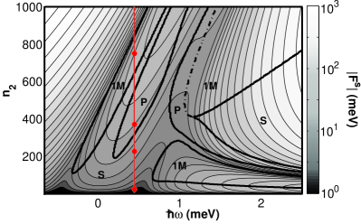
Figure 1: Energy-intensity ($\hbar\omega$-$n_{2}$) diagram. The colour scale corresponds to increasing values of $|F^{s}|$ in logarithmic scale and the thin isolines are geometrically spaced contour lines. The thick black line separates the stability (S) regions from instability ones: depending on their character, these are marked by either 1M (one-mode instability) or P (parametric instability). The dash-dot line separates a one-mode instability region from a parametric instability one. The dots on the vertical $\hbar\omega=0.45\,\textrm{meV}$ line correspond to the pump parameters used later on in Figs. 7 and 8. The system parameters are inspired from the symmetric double-box polariton traps discussed in Sec. VI, namely $J=0.5~{}\mbox{meV}$, $\gamma_{1}=\gamma_{2}=\gamma=0.2~{}\mbox{meV}$, $g=1.1~{}\times~{}10^{-3}~{}\mbox{meV}$, $\omega_{1}=\omega_{2}$.

The phase diagram is determined from the stability of the stationary state (5). The black thick lines mark the contours between the regions of stability and the regions of instability, as obtained by solving the linearized problem Eq. (12). Here, regions of one-mode instability or parametric instability are indicated by respectively 1M and P following the definitions introduced in Sec. II.2.

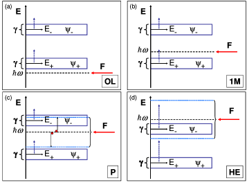
Figure 2: Scheme of the effective energy levels $E_{\pm}$ of a two mode model under a continuous-wave pump. The vertical dashed arrows indicate the nonlinear blue-shift. The horizontal solid arrows indicates the pump energy $\hbar\omega$ in the different regimes discussed in the text: (a) Optical limiter; (b) One-mode instability; (c) Parametric instability; (d) High-energy pumping.

For very small pump amplitudes, two resonances are clearly visible in Fig. 1. As explained in Sec. II, they corresponds to the $\psi_{\pm}$ eigenmodes of the linearly coupled system and lye at exactly $\hbar\omega=\pm J$. The linewidth has been taken smaller than the linear coupling $\gamma/2<J$, so the corresponding lines are well distinct.

For increasing values of the pump amplitude, the resonances of the system are modified by the nonlinearity (see the scheme in Fig. 2). At moderate pump amplitudes for which $g\,n_{1,2}<J,\gamma$, the main effect of the nonlinearity is a blue-shift of the two resonances. On the other hand, several different instability mechanisms can take place at larger pump amplitudes depending on the pump energy $\hbar\omega$.

III.1 Optical Limiter

For $\hbar\omega<-J$, the pump energy lies below the two energy levels: this configuration, often called optical limiter (OL) in the literature NLO , is stable for all pump intensities. As shown in the sketch in Fig. 2(a), the effective energy levels are in fact pushed even further off resonance from the pump by the nonlinear blue-shifts.

III.2 Optical bistability

For a pump energy just above the lower energy $+$ mode (i.e. $\hbar\omega\gtrsim-J$), the nonlinear shift is able to push the effective energy level into resonance with the pump (see Fig. 2(b)) and give rise to a single mode (1M), saddle-node cross instability. Analogous behaviour takes place for pump energies just above the higher energy $-$ mode (i.e. for $\hbar\omega\gtrsim J$).

The occurrence of regions of one-mode instability for energies higher than a mode resonance is a well studied subject in the general literature on instabilities halebook . Concerning nonlinear optical systems, it has been extensively studied both in the simplest case of single cavities NLO , as well as in more complex cases of coupled optical cavities lugiato_review ; iaccouplcav and OPOs baas_bistab ; gippius04 ; wouters07a .

As a general feature halebook , one-mode instabilities of this kind often give rise to bistable behaviors, i.e. the coexistence of several stable solutions for the same values of the pump energy and amplitude. An example of this behaviour is shown in Fig. 3 where the dependence of the intensities $n_{1,2}$ on the pump amplitude is plotted for a pump energy just above the lower resonance.

An hysteresis cycle is apparent: as the pump amplitude $F$ increases from zero, the system moves along the lower branch of stable solutions until its end point is reached. Only at this point the system jumps on the upper branch. If the pump amplitude is then decreased, the system keeps moving along the upper branch of stable solution until its end point is reached, where it jumps back to the lower branch.

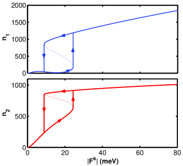
Figure 3: Intensities $n_{1}$ (panel (a)) and $n_{2}$ (panel (b)) as a function of the pump amplitude. Pump energy $\hbar\omega=0.45~{}\mbox{meV}$. The arrows highlight the hysteresis cycle due to optical bistability. Same system parameters as in Fig. 1.

III.3 Parametric instability

For a pump energy between the two resonances, a parametric instability appears. When the pump energy equals the average of the effective energies $(E_{+}+E_{-})/2$, the parametric process NLO sketched in Fig. 2(c) where the pump field creates a signal $+$ and an idler $-$ fields becomes resonant. This happens within the window $\gamma_{j}<\hbar\omega<J+gn_{2}$, where the stationary solutions are stable for small pump amplitudes, but become parametrically unstable as soon as the parametric gain is able to overcome the losses $gn_{2}>\gamma_{j}$. Note that the effect of $n_{1}$ can be neglected here, as in the considered energy window one has $n_{1}\ll n_{2}$ (see Fig. 5). In the dynamical systems language, such an instability is called a Hopf bifurcation cross .

The strong amplification of fluctuations around the stationary solution eventually results in a self-pulsing dynamics where the system keeps on oscillating for indefinite times. From a different point of view, these oscillations can be seen as the result of the interference between three fields at different frequencies, i.e. the pump, signal, and idler fields of the parametric oscillator NLO ; Ciuti_review . This behavior will be discussed in better detail in the next section.

III.4 High-energy region

For pump energy exceeding the energy of both resonances, several instability regions are expected to appear as a consequence of the complex interplay of single-mode 1M and parametric P instabilities. Both effective energy levels eventually cross the pump energy, as well as the parametric resonance [Fig. 2(d)]. The diagram in Fig. 1 is therefore much richer in this window: for a given pump energy $\hbar\omega$ and increasing values of $n_{2}$, three regions of one-mode instability and three regions of parametric instability can be identified, as well as a thin stability region in between the first 1M and P regions.

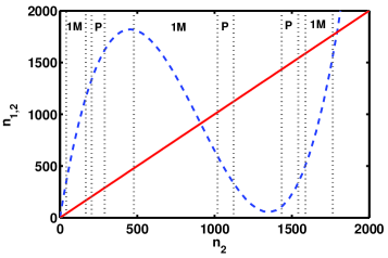
Figure 4: Intensity $n_{1}$ as a function of $n_{2}$ for a high pump energy $\hbar\omega=1.5~{}\mbox{meV}$ (dashed line). The solid line corresponds to $n_{2}$ and is a guide for the eye in order to identify the regions where $n_{1}\gg n_{2}$, $n_{1}\approx n_{2}$ or $n_{2}\gg n_{1}$. Separation between instability regions of different (1M or P) kinds are indicated by the vertical dotted lines. Same system parameters as in Fig. 1.

To understand the origin of the different regimes, the intensities $n_{1,2}$ are plotted in Fig. 4 as a function of $n_{2}$ for $\hbar\omega=1.5~{}\mbox{meV}$. The behaviour is quite complex, yet can be analytically interpreted from Eq. (6), which indeed gives

$$n_{1}=J^{-2}\left[(gn_{2}-\hbar\omega)^{2}+\frac{\gamma_{2}^{2}}{4}\right]n_{2}\,.$$ (13)

For a pump energy lying between the two blue-shifted resonances, i.e. $-J+gn_{2}<\hbar\omega<J+gn_{2}$, the intensity $n_{2}$ of the non-pumped mode is larger than the intensity $n_{1}$ of the pumped one, i.e. $n_{2}>n_{1}$. Conversely, for either lower ($\hbar\omega<-J+gn_{2}$) or larger ($\hbar\omega>J+gn_{2}$) pump energies, the pumped mode has a larger intensity. This trend is illustrated in the $n_{1}/n_{2}$ plot shown in Fig. 5.

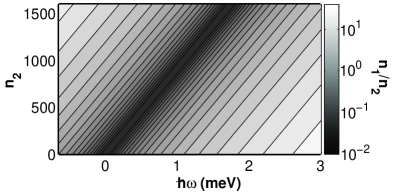
Figure 5: Logarithmic gray-scale plot of the ratio $n_{1}/n_{2}$ as a function of the pump energy and of the value $n_{2}$. Same parameters as in Fig. 1.

First we investigate the region around the stability tongue extending at $\hbar\omega\gtrsim 1.5~{}\mbox{meV}$ for relatively small values of $F$. While the energy of the pumped $1$ mode is significantly blue-shifted by the nonlinear term, the non-pumped $2$ mode remains almost empty (see Fig. 4). The two $1,2$ modes are then far in energy, so the effect of the linear coupling is strongly suppressed. The nearby 1M instability region then corresponds to the bistability loop for a pump close to resonance with the higher energy mode, which in this region basically coincides with the blue-shifted $1$ mode. The physics is analogous for the second 1M instability region located just above.

The third 1M instability at much larger pump amplitudes corresponds to the opposite situation where the $2$ mode has been shifted above $\hbar\omega$ and consequently $n_{2}\gg n_{1}$ according to (13). The bistability loop then involves the lower resonance, which in this regime basically corresponds to the unperturbed $1$ mode.

We finally consider the intervals of parametric instability. The first and the third intervals correspond to resonant scattering processes taking place in a regime where the modes are effectively decoupled as $n_{1}\gg n_{2}$ or $n_{2}\gg n_{1}$, respectively. In these regimes, the two $\pm$ eigenmodes essentially coincide with the $1,2$ modes. The second interval corresponds instead to an intermediate regime where $n_{1}\approx n_{2}$, and the two $\pm$ eigenmodes are a superposition of both $1,2$ modes.

III.5 The spectrum of fluctuations around the stationary solution

The stability properties of the stationary solution discussed in the previous section are further illustrated by looking at the eigenvalues of the Bogoliubov linearized theory (12) of small fluctuations around the stationary state Ciuti_review ; iac_superfl . These are plotted in Fig. 6 as a function of the intensity $n_{2}$ of the non-pumped mode for the case of a pump energy $\hbar\omega$ chosen between the $\pm$ eigenmodes of the unloaded system.

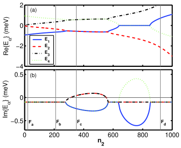
Figure 6: Real (a) and imaginary (b) part of the linearized spectrum around the steady state solution as a function of $n_{2}$. Stable regions correspond to the imaginary part of the spectrum being negative. Pump frequency $\hbar\omega=0.45~{}\mbox{meV}$. The vertical lines indicate the $n_{2}$ values used in the panels (a-d) of Figs. 7 and 8. Same system parameters as in Fig. 1.

In the linear $n_{1,2}\rightarrow 0$ regime, the frequencies and damping rates tend to the ones $\mbox{Re}\{E_{3,1}\}=-\mbox{Re}\{E_{4,2}\}=\pm J/2-\hbar\omega$, $-\mbox{Im}\{E_{1,2,3,4}\}=\gamma/2$ of the unloaded system. As a consequence of interactions, the frequency $\mbox{Re}\{E_{1,3}\}$ of the positive-weighted Bogoliubov modes are blue-shifted for growing intensities, while the ones $E_{2,4}$ of the negative-weighted ones are red-shifted: this makes them to pairwise intersect at some value of the intensity. Here, each pair collapses onto values $\mbox{Re}\{E_{2(4)}\}=\mbox{Re}\{E_{1(3)}\}$ opposite in sign. Correspondingly, the damping rate increases $-\mbox{Im}\{E_{1}\}=-\mbox{Im}\{E_{4}\}>\gamma/2$ for two of them, while it decreases $-\mbox{Im}\{E_{2}\}=-\mbox{Im}\{E_{3}\}<\gamma/2$ for the two others, possibly giving rise to a dynamical instability, as in the case displayed in the figure. The fact that frequencies of the modes involved in the instability are non-zero is a signature of the parametric nature of the instability.

For larger intensities, the frequencies split again within a narrow intensity interval where the damping rate goes back to $\gamma/2$, but another instability region occurs at even higher intensities as a consequence of the intersection $\mbox{Re}\{E_{1}\}=\mbox{Re}\{E_{4}\}$: while the the imaginary parts of the $2,3$ modes stay unchanged, the ones of the $1,4$ modes are split and dynamical instability is signalled by one of them becoming positive. Since the unstable mode has zero frequency, the instability has the one-mode character typical of optical bistability loops.

For even larger intensities, the stationary state becomes stable again: because of the large blue- (red-) shift of the positive (negative)-weighted Bogoliubov modes, no further intersections of the mode frequencies can in fact occur.

IV Continuous pump: bistability, self-pulsing, and response to a probe

The stationary states and the stability regions identified in the previous section are a good starting point for the dynamical study of the system that we carry out in the present section by numerically solving Eqs. (1-2). We first investigate the onset of the steady state when the pump intensity is slowly increased in time to its asymptotic value. Then we characterize the response of the system in its steady state to an additional probe: this provides a simple and effective way of measuring the frequencies and damping rates of the Bogoliubov modes in the different regimes.

The quasi-continuous pump is assumed to have a smooth temporal profile of the form

$$F(t)=F_{max}\left(1-\frac{2}{1+e^{(t/\tau)^{2}}}\right)\,.$$ (14)

For very long switch-on time, the system evolves in a quasi-static way through a sequence of stable stationary states.

Once the system has got to its asymptotic stationary solution, a weak and short probe pulse is applied onto mode $1$. Its temporal shape is assumed to be a Gaussian

$$f_{g}(t)=f_{g}^{0}e^{-(t-t_{0})^{2}/\tau_{g}^{2}}\,,$$ (15)

its central frequency coincides with the one of the continuous pump, and its duration $\tau_{g}$ is chosen to be short enough for the pulse to encompass all the relevant spectral features, i.e. all the 4 Bogoliubov modes shown in Fig. 6.

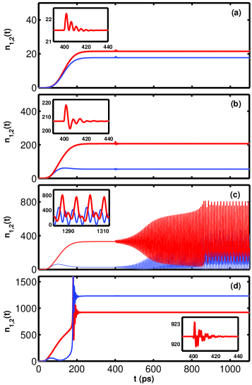
Figure 7: Time-evolution of the $n_{1}(t)$ (dashed line) and $n_{2}(t)$ (solid line) intensities for growing pump amplitudes $F_{max}=1\,\mbox{meV}$ (a), $5\,\mbox{meV}$ (b) $8\,\mbox{meV}$ (c), $20\,\mbox{meV}$ (d). Pump energy $\hbar\omega=0.45~{}\mbox{meV}$. Pump switch-on time $\tau=100~{}\mbox{ps}$. Probe amplitude $f_{g}^{0}=10^{-2}\,F_{max}\ll F_{max}$, probe duration $\tau_{g}=0.3\,\mbox{ps}\ll\pi\,\hbar/J$, probe delay $t_{0}=400\,\mbox{ps}\gg\tau$. Same system parameters as in Fig. 1. The pump parameters used for panels (a-d) correspond to the red dots in Fig. 1.

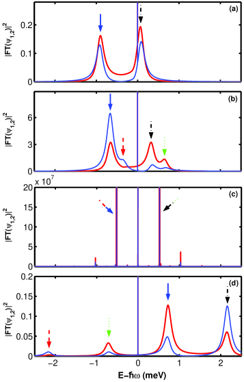
Figure 8: Fourier transform spectra of $\psi_{1}$ (dashed line) and $\psi_{2}$ (solid line) for growing pump amplitudes $F_{max}=1,\,5,\,8,\,20~{}\mbox{meV}$. The central $\delta$-peak is at the pump frequency. The arrows indicate the frequencies of the Bogoliubov modes with the same colour code as in Fig. 6. Parameters of the (a-d) panels correspond to the ones in Fig. 7.

Numerical predictions for $n_{1,2}(t)$ are shown in Fig. 7 for the different regimes. The quasi-cw pump energy $\hbar\omega$ is taken to be between the linear resonance peaks and increasing values of the pump amplitude $F$ are chosen for the different panels (see dots in Fig. 1). The corresponding spectra shown in Fig. 8 are obtained by Fourier transform of $\psi_{1,2}(t)$. In order to eliminate complications due to the switch-on dynamics, we have restricted the Fourier transform to the temporal window following the arrival of the probe pulse. The central $\delta$-peak corresponds to the pump frequency.

IV.1 Stable regime

For small values of the asymptotic pump amplitude $F_{max}$ [Fig. 7(a) and (b)], the evolution during the switch-on time smoothly leads the system to the asymptotic stationary state. As this solution is stable, the response to the probe pulse gets quickly damped within a time-scale of the order of ten picosecond. While for very small intensities (Fig. 7(a)) the response consists of damped oscillations at a single frequency, for larger intensities (Fig. 7(b)) relaxation is more complex and involves interference of more frequencies.

This difference is apparent in the corresponding spectra shown in Fig. 8(a,b) which are to be compared to the Bogoliubov modes shown in Fig. 6. Well inside the stability region, only the positive-weighted Bogoliubov modes with a significant $U$ component [see Eq. (10)] are in fact visible. On the other hand, when the parametric instability region is approached, the normal components $U$ are significant for all modes and all the four frequencies become then visible in the spectrum (see Fig. 8(b)). As usual, the finite linewidth of the peaks is fixed by the finite and negative imaginary part of the Bogoliubov modes, i.e. by their damping rate. In the present case, this is the same for all Bogoliubov modes.

IV.2 Parametric instability

The physics is richer in Figs. 7(c) and 8(c) where a larger pump amplitude $F_{max}=8$ meV is considered: in this case, the asymptotic stationary state is in fact parametrically unstable. As the pump intensity is increased very smoothly, the system adiabatically follows the stationary state at the instantaneous value of $F$ even in the unstable region. However, the arrival of the probe pulse speeds up the onset of the instability: the perturbation that it induces is quickly amplified until the system gets to the self-pulsing regime where undamped periodic oscillations take place for indefinite time. Their frequency is close to the one of the linear Bogoliubov mode getting unstable. Correspondingly, two $\delta$-peaks appear in the spectrum shown Fig. 8(c) at energies $E-\hbar\omega=\pm 0.52~{}\mbox{meV}$. The weaker $\delta$-peaks at harmonic frequencies contribute to the quite complex waveform of the self-pulsing oscillations in time shown in Fig. 7(c).

IV.3 One-mode instability

To highlight hysteresis phenomena, we now choose an asymptotic value of the pump amplitude above the jump-up threshold of the bistability loop shown in Fig. 3. The switch-on then does not take place in a smooth way and the system has to perform a sudden jump when the end-point of the lower branch is reached: among the many complex behaviour that may take place wouters07a , the behaviour of the present system is the simplest: it jumps to the higher-intensity branch of the bistable loop. Once these upper branch is reached, the system is stable again and the response to the probe pulse is qualitatively similar to the case of panels (a,b). The only difference is the higher frequency of the oscillations, and the presence of three different excitation frequencies which contribute to the complex relaxation dynamics: one negative-weighted Bogoliubov mode has in fact a significant $U$ component.

V Pulsed excitation: Josephson oscillations and self-trapping

After having investigated the behaviour of the system under a continuous pump, it is now interesting to look at the case where only a pulsed pump is applied to the system. Specifically, we numerically solve Eqs. (1-2) using a Gaussian temporal profile for the pump

$$F(t)=F_{max}\,e^{-(t-t_{p})^{2}/\tau_{p}^{2}}\,.$$ (16)

The duration $\tau_{p}$ of the pump pulse is taken to be very short as compared to all time scales of the system dynamics: the system is then almost istantaneously excited by a sudden kick, and then let evolve and relax without any further pumping. The results are summarized in Fig. 9(a,c,e,g) in the time domain, while the corresponding Fourier spectra are shown in Fig. 9(b,d,f,h).

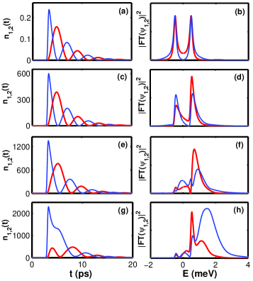
Figure 9: Intensity dynamics (a,c,e,g) and corresponding Fourier spectra (b,d,f,h) under a Gaussian pulsed pump (Eq. (16)) at time $t_{p}=3\,\mbox{ps}$ of duration $\tau_{p}=0.2\,\mbox{ps}$. Peak pump amplitude $F_{max}=1~{}\mbox{meV}$ (a,b), $50~{}\mbox{meV}$ (c,d), $75~{}\mbox{meV}$ (e,f) and $100~{}\mbox{meV}$ (g,h). Blue (red) lines corresponds to the $1$ ($2$) modes. Spectra are obtained by Fourier transforming the signals in the whole time interval. Same system parameters as in Fig. 1.

For low pump amplitudes in the linear regime, the intensities in the two wells manifest Josephson-like oscillations [Fig. 9(a)]. The pump pulse creates in fact a localized excitation in the $1$ mode, which is a superposition of the symmetric and anti-symmetric eigenmodes of the system. Because of their energy splitting, the system shows complete Josephson oscillations with a period $\pi\hbar/J$, which then damp out at a rate $\gamma$ under the effect of losses. Correspondingly, the Fourier spectrum shown in Fig. 9(b) is characterized by a pair of resonance peaks split by $2J$.

For stronger pump amplitudes, the instantaneous intensity in the system increases, and eventually results in significant nonlinear effects. While the time evolution of the intensities [Fig. 9(c)-(e)] does not appear to be significantly modified, nonlinear effects are visible in the spectra of Fig. 9(d)-(f) already at moderate intensities as a global blue-shift of the spectrum and a significant increase of the width of the peaks. In particular, in Fig. 9(f), note how the blue-shift of the spectrum relative to the field $\psi_{1}$ is larger than the blue-shift of the spectrum relative to $\psi_{2}$: this is due to the fact that the intensity $n_{1}$ is at short times much larger than the intensity $n_{2}$. In the Fourier spectrum of $\psi_{1}$, we also clearly recognize two peaks at $J=\pm 0.5\,\textrm{meV}$ corresponding to the eigenfrequencies of the linear dynamics that is recovered at long times once the intensities have dropped to small values. Similar peaks also contribute to the Fourier spectrum of $\psi_{2}$, but are hardly visible in the figure, their weak intensity being hidden by the tails of the main peaks.

The appearance of peaks at frequencies characteristic of the nonlinear regime is a precursor of the self-trapping regime that appears for stronger pump amplitudes: in this case, the nonlinear effects are in fact dominant in determining both the spectrum and the time evolution of the intensities [Fig. 9(g)-(h)].

In the early stages of the evolution when the intensity is the largest, nonlinear effects dramatically suppress the amplitude of Josephson oscillation: most of the intensity is in fact self-trapped in the mode $1$ and the intensity of mode $2$ oscillates around a much smaller value. As time goes on, the total intensity slowly drops under the effect of losses and eventually complete Josephson oscillations are recovered: the transition between the self-trapping regime and Josephson oscillations can be located in the vicinity of the time when the total intensity equals the critical density $n_{1}+n_{2}=n^{c}_{tot}=4J/g$ of equilibrium Josephson systems josephson_th . The presence of losses is only responsible for a small shift of the critical point.

Consequences of this physics can be observed also in Fig. 9(h): both spectra show in fact two broad peaks centered at high energies (i.e. at $E\simeq 0$ and $E\simeq 1.5~{}\mbox{meV}$), which represent the two resonances of the system in the self-trapping regime, and two lower energy peaks at $E=\pm J=\pm 0.5\,\textrm{meV}$, representing the frequencies of the Josephson oscillations. These two latter peaks are asymmetric [differently from the pure linear regime displayed in Fig. 9(b)] because the dynamics has been modified by the occurrence of the self-trapping regime.

VI Microcavity polariton boxes

In this last section we show how the parameters of the two-mode model can be evaluated from the microscopic structure of a specific physical system. On one hand we demonstrate that all the physics discussed in the previous sections can actually be observed in realistic systems, on the other hand we confirm the quantitative validity of the predictions of the two-mode model by comparing them to a full numerical integration of the generalized Gross-Pitaevskii equation for polaritons Ciuti_review ; iac_superfl .

Although many other configurations based on e.g. coupled DBR cavities are available to study Josephson-like effects in an optical context lugiato_review ; iaccouplcav ; carole ; trombettoni , our attention will be concentrated on the specific case of double-well polariton traps. Such a system was recently realized eldaif06 ; kaitouni06 and combines the strong nonlinearity due to the excitonic component of the polariton to the possibility of a micron-scale spatial confinement by laterally patterning the thickness of the cavity layer. From the point of view of Josephson physics, this geometry is very attractive as it allows independent collection of light emitted from the two boxes and preserves the signal from being covered by the incident laser field.

VI.1 From the non-equilibrium GPE to the two mode model

The dynamics of the macroscopic polariton field $\Psi({\bf r},t)$ is described at mean-field level by a non-equilibrium generalization of the Gross-Pitaevskii equation (GPE) of the form Ciuti_review ; iac_superfl :

$$i\hbar\,\frac{d}{dt}{\Psi}\left({\bf r},t\right)=\left(-\frac{\hbar^{2}\nabla^{2}}{2m_{p}}+U_{ext}\left({\bf r}\right)-i\frac{\gamma}{2}\right)\Psi\left({\bf r},t\right)\\ +v\,\left|\Psi\left({\bf r},t\right)\right|^{2}\Psi\left({\bf r},t\right)+f\left({\bf r},t\right)\,.$$ (17)

$m_{p}$ is the effective mass of the lower polariton, $\gamma$ is the decay rate, $U_{ext}$ is the trapping potential, $v$ is the effective polariton mutual interaction rochat00 ; ben01 ; okumura02 and $f({\bf r},t)$ is the amplitude of the coherent pump field.

In this paper, we consider the case of a trapping potential $U_{ext}({\bf r})$ formed by two adjacent wells, as displayed in Fig. 10(a):

$$U_{ext}=-U_{0}\,\theta\left(L_{y}-\left|y\right|\right)\left[\theta\left(L_{x}+{\delta}/{2}-x\right)\,\theta\left(x-{\delta}/{2}\right)\right.\\ +\left.\theta\left(L_{x}+{\delta}/{2}+x\right)\,\theta\left(-x-{\delta}/{2}\right)\right]\,.$$ (18)

For this potential, the fundamental mode of energy $E_{gs}$ is described by an eigenfunction $\phi_{gs}({\bf r})$ which is symmetric in the two wells (see Fig. 10(b)), while the first excited mode of energy $E_{exc}$ corresponds to an antisymmetric eigenfunction $\phi_{exc}({\bf r})$ (see Fig. 10(c)). Without loss of generality, both these functions can be taken real.

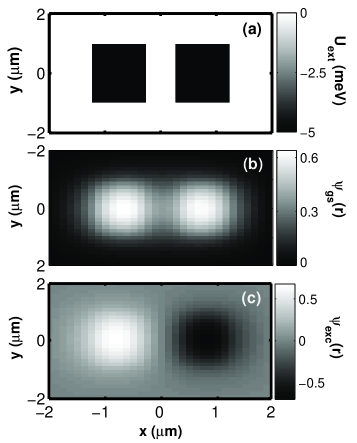
Figure 10: Trapping potential $U_{ext}$ (Eq. (18) due to two adjacent rectangular wells (a), and the fundamental $\phi_{gs}({\bf r})$ (b) and first excited $\phi_{exc}({\bf r})$ (c) modes of the corresponding equilibrium GPE (31). The spatial profiles are displayed in grey tones.

The pump field is considered to be monochromatic, with a gaussian spatial profile

$$f({\bf r},t)=2\pi\,\sigma^{2}\,f_{0}\,e^{-|{\bf r}-{\bf r_{1}}|^{2}/\sigma^{2}}\,e^{-i\omega t}$$ (19)

centered on the first well at ${\bf r_{1}}=((L_{x}+\delta)/2,L_{y}/2)^{t}$. Provided the pump energy is close to $E_{gs}$ and $E_{exc}$ and all other excited modes of the trapping potential are at much higher energies, the coherent field $\Psi({\bf r},t)$ can be safely written in the two-mode limit josephson_th as a time-dependent superposition of the two lower energy modes $\phi_{gs}({\bf r})$ and $\phi_{exc}({\bf r})$ only.

For the present case, it is useful to write the superposition in the form

$$\Psi\left({\bf r},t\right)=\psi_{1}\left(t\right)\phi_{1}\left({\bf r}\right)+\psi_{2}\left(t\right)\phi_{2}\left({\bf r}\right),$$ (20)

where the Wannier-like functions

$$\phi_{1,2}\left({\bf r}\right)=\frac{1}{\sqrt{2}}\left[\phi_{gs}\left({\bf r}\right)\pm\phi_{exc}\left({\bf r}\right)\right]$$ (21)

are mostly localized in each well and orthogonal to each other.

By substituting Eq. (20) in Eq. (17) and then projecting onto the lowest states, two coupled dynamical equations for the amplitudes $\psi_{1,2}(t)$ are obtained of the form:

$$i\hbar\dot{\psi}_{j}=\left(\hbar\omega_{j}-i{\gamma}/{2}\right)\psi_{j}+g\,|\psi_{j}|^{2}\psi_{j}-J\psi_{3-j}\\ +b\left[\left(2|\psi_{j}|^{2}+|\psi_{3-j}|^{2}\right)\psi_{3-j}+\psi_{3-j}^{*}\psi_{j}^{2}\right]\\ +c\left(2|\psi_{3-j}|^{2}\psi_{j}+\psi^{*}_{j}\psi^{2}_{3-j}\right)+F_{j}(t).$$ (22)

Linear dynamics is summarized by the diagonal term

$$\hbar\omega_{j}=\frac{1}{2}\left(E_{gs}+E_{exc}\right)\,,$$ (23)

and the linear hopping coefficient

$$J=\frac{1}{2}\left(E_{exc}-E_{gs}\right)\,.$$ (24)

Pumping is described by

$$F_{j}(t)=\int d{\bf r}\,\phi_{j}({\bf r})\,f({\bf r},t)\,,$$ (25)

while nonlinear effects are described by the three coupling coefficients

$$g = v\int d{\bf r}\left[\phi_{1,2}({\bf r})\right]^{4}$$ (26)

$$b = v\int d{\bf r}\phi_{2,1}({\bf r})\left[\phi_{1,2}({\bf r})\right]^{3}$$ (27)

$$c = v\int d{\bf r}\left[\phi_{1}({\bf r})\right]^{2}\left[\phi_{2}({\bf r})\right]^{2}\,,$$ (28)

For typical geometries and for moderate intensities, the coefficients $b$ and $c$ are much smaller than the other quantities and can be safely neglected. Within this approximation, Eq. (22) reduces to the two mode model Eqs. (1-2) used in the previous Sections.

VI.2 Comparison with the 2-mode model

In order to verify the validity of the two-mode approximation, a numerical integration of the full GPE Eq. (17) can be performed and then quantitatively compared to the predictions of the two-mode model.

For this comparison, realistic parameters for typical polariton boxes in GaAs based microcavities eldaif06 ; kaitouni06 are used, that is a trapping potential depth $U_{0}=5~{}\mbox{meV}$, lateral box sizes $L_{x}=1~{}\mu\mbox{m}$ and $L_{y}=2~{}\mu\mbox{m}$, a polariton mass $m_{p}=7\times 10^{-5}m_{0}$ ($m_{0}$ being the electron mass) and a nonlinear coupling constant $v=2\times 10^{-3}~{}\mbox{meV}\mu\mbox{m}^{2}$. We assume the separation $\delta=0.5~{}\mu\mbox{m}$ between the two wells. The corresponding potential $U_{ext}$ and the functions relative to the first two GP modes are displayed in Fig. 10. A spatial width $\sigma=0.5~{}\mu\mbox{m}$ is taken for the pump spot.

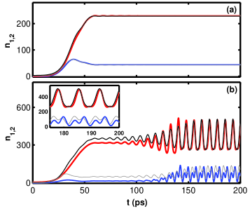
Figure 11: Dynamical evolution of $n_{1}$ and $n_{2}$ ($n_{2}>n_{1}$), as obtained from the full numerical calculation of GPE (thin lines) and from the two-mode model (thick lines). Panel (a): GPE simulations with pump energy $\hbar\omega=-2.8~{}\mbox{meV}$ and pump amplitude $f_{0}=5~{}\mbox{meV}$; parameters of the corresponding effective two-mode model: $\hbar\omega_{1,2}=-3.15~{}\mbox{meV}$, $J=0.45~{}\mbox{meV}$, $g=10^{-3}~{}\mbox{meV}$ and $F_{1}=5.8~{}\mbox{meV}$. Panel (b): GPE simulations with pump energy $\hbar\omega=-2.8~{}\mbox{meV}$ and pump amplitude $f_{0}=7.5~{}\mbox{meV}$; parameters of the corresponding effective two-mode model: $\hbar\omega_{j}=-3.1~{}\mbox{meV}$, $J=0.5~{}\mbox{meV}$, $g=10^{-3}~{}\mbox{meV}$ and $F_{1}=8.5~{}\mbox{meV}$.

The time-evolution of the polariton occupation $n_{1,2}(t)=|\psi_{1,2}(t)|^{2}$ in the two wells is plotted in Fig. 11. In the present GPE framework, the occupations $n_{1,2}$ of each of the two wells are defined by the spatial integrals

$$n_{1}(t)=\int_{0}^{+\infty}\!\!\!\!\!dx\int\!dy\,\,|\Psi({\bf r},t)|^{2}$$ (29)

$$n_{2}(t)=\int_{-\infty}^{0}\!\!\!\!\!dx\int\!dy\,\,|\Psi({\bf r},t)|^{2}.$$ (30)

Two different parameter choices are made in the two panels of Fig. 11. In (a), the system tends to a stable stationary state, while self-pulsing oscillations are visible in (b). The qualitative agreement with respectively panels (a,b) and (c) of Fig. 7 is apparent. Note that the switch-on time of the pump considered in Fig. 11 is not long enough to guarantee a quasi-static evolution of the system even in the unstable region: differently from Fig. 7(c), the self-pulsing oscillations are immediately visible without the need of a perturbation seed.

As the linear coupling $J$ is very sensitive to the shape of the wavefunctions in the barrier, interactions may affect it quite significantly, spoiling the quantitative agreement with the two-mode model. In order to get a good quantitative agreement in all regimes, a better approximation can be adopted for the localized wavefunctions using for $\phi_{gs}({\bf r})$ and $\phi_{exc}({\bf r})$ the two lowest-energy solutions of the time-independent, equilibrium Gross-Pitaevskii equation:

$$\left(-\frac{\hbar^{2}\nabla^{2}}{2m_{p}}+U_{ext}\left({\bf r}\right)+v\,N\,\left|\phi\left({\bf r}\right)\right|^{2}\right)\,\phi\left({\bf r}\right)=E^{(N)}\,{\phi}\left({\bf r}\right).$$ (31)

The total polariton number $N=n_{1}+n_{2}$ has to be obtained from the long-time limit $t\rightarrow\infty$ of the full GP equation once the solution has come to their asymptotic steady state, or by averaging over the period of the self-pulsing oscillations. Correspondingly, Eqs. (23) and (24) have to be substituted by the N-dependent equations

$$\hbar\omega_{j} = \frac{1}{2}\left(E_{gs}^{(N)}+E_{exc}^{(N)}\right)+$$ (32)

$$-\frac{vN}{2}\int d{\bf r}\left([\phi_{gs}({\bf r})]^{4}+[\phi_{exc}({\bf r})]^{4}\right)\,$$

and

$$J=\frac{1}{2}\left(E_{exc}^{(N)}-E_{gs}^{(N)}\right)\,,$$ (33)

respectively. As expected, the main effect of interactions is to slightly lift the bottom of the two wells, so to effectively reduce the barrier height and enhance tunneling.

The result of such a procedure is also shown in Fig. 11: the overall qualitative agreement is good. From a quantitative point of view, the agreement is always excellent in the stable regime of panel (a), while some discrepancies are visible in panel (b), in particular at short times before the self-pulsing sets in. This can be expected, as the parameters of the two-mode model extracted from the late time dynamics slightly differ from what one would get from the early stages. Furthermore, the spatial profile of the wavefunction has a significant variation in time during the self-pulsing dynamics.

VII Conclusions

In this paper we have studied the two-mode dynamics of spatially coupled polariton boxes under a coherent external pumping and we have shown that this provides an interesting non-equilibrium optical generalization of the well-known Josephson effect of weakly coupled superfluids and superconductors.

For a continuous wave pumping, a phase diagram has been obtained which summarizes the steady state of the system as a function of pump intensity and frequency. Stable and unstable regions have been identified; one-mode and parametric instabilities have been shown to be intrinsecally related to respectively optical bistability and self-pulsing effects. The response of the system to an additional probe provides unambiguous information on the Bogoliubov modes around the stationary state.

For a short pump pulse, the crossover from a Josephson oscillations regime to a self-trapping one has been characterized as a function of the pump intensity. Peculiar features due to the non-equilibrium nature of the system have been pointed out.

The validity of the two-mode model and the actual observability of the predicted effects has been verified on the basis of the non-equilibrium Gross-Pitaevskii equation for polaritons in a double-well trap potential using parameters inspired by recent experiments.

D. S. and V. S. acknowledge financial support from the Swiss National Foundation through Project No. PP002-110640. IC is grateful to C. Ciuti, A. Recati, and A. Trombettoni for continuous stimulating discussions.

References

- (1) Special issue on Microcavities, edited by J. Baumberg and L. Viña [Semicond. Sci. Technol. 18, S279-S434 (2003)].
- (2) Physics of Semiconductor Microcavities, edited by B. Deveaud, special issue of Phys. Stat. Sol. B, 242, 2145 (2005).
- (3) C. Ciuti, P. Schwendimann, and A. Quattropani, Semicond. Sci. Technol. 18, S279-S293 (2003).
- (4) J. Keeling, F. M. Marchetti, M. H. Szymanska, P. B. Littlewood, Semicond. Sci. Technol. 22, R1-R26 (2007)
- (5) I. Carusotto and C. Ciuti, Phys. Rev. Lett. 93, 166401 (2004); C. Ciuti and I. Carusotto, Phys. Stat. Sol. (b) 242, 2224 (2005).
- (6) M. Wouters and I. Carusotto, Phys. Rev. B 74, 245316 (2006)
- (7) M. H. Szymańska, J. Keeling, P. B. Littlewood, Phys. Rev. Lett. 96, 230602 (2006)
- (8) M. Wouters and I. Carusotto, Phys. Rev. Lett. 99, 140402 (2007).
- (9) M. Bayer, T. Gutbrod, A. Forchel, T. L. Reinecke, P. A. Knipp, R. Werner, and J. P. Reithmaier, Phys. Rev. Lett. 83, 5374 (1999).
- (10) G. Dasbach, M. Schwab, M. Bayer, and A. Forchel, Phys. Rev. B 64, 201309(R) (2001).
- (11) A. Loeffler, J. P. Reithmaier, G. Sek, C. Hofmann, S. Reitzenstein, M. Kamp, and A. Forchel, Appl. Phys. Lett. 86, 111105 (2005).
- (12) O. El Daïf, A. Baas, T. Guillet, J.-P. Brantut et al., Appl. Phys. Lett. 88, 061105 (2006).
- (13) R. I. Kaitouni et al., Phys. Rev. B 74, 155311 (2006).
- (14) D. Bajoni, E. Peter, P. Senellart, J. L. Smirr, I. Sagnes, A. Lema tre and J. Bloch, Appl. Phys. Lett. 90, 051107 (2007)
- (15) R. Balili, V. Hartwell, D. Snoke, L. Pfeiffer, and K. West, Science 316, 1007 (2007).
- (16) L.P. Pitaevskii and S. Stringari, Bose-Einstein Condensation (Clarendon Press, Oxford, 2003).
- (17) G.J. Milburn et al., Phys. Rev. A 55, 4318 (1997); A. Smerzi et al., Phys. Rev. Lett. 79, 4950 (1997); S. Giovanazzi et al., Phys. Rev. Lett. 84, 4521 (2000).
- (18) M. Albiez et al., Phys. Rev. Lett. 95, 010402 (2005).
- (19) L.A. Lugiato, M. Brambilla and A. Gatti, Adv. At. Mol. Opt. Phys. 40, 229 (1998).
- (20) I. Carusotto and G. C. La Rocca, Phys. Lett. A 243, 236 (1998).
- (21) I. Carusotto, G. C. La Rocca, Phys. Rev. B 60, 4907 (1999).
- (22) A. Verger, C. Ciuti, and I. Carusotto, Phys. Rev. B 73, 193306 (2006).
- (23) P. N. Butcher and D. Cotter, The elements of nonlinear optics (Cambridge University Press, Cambridge, 1993); R. W. Boyd, Nonlinear optics (Academic Press, San Diego, 1992).
- (24) M. C. Cross and P. C. Hohenberg, Rev. Mod. Phys. 65, 851 (1993).
- (25) J. Hale and H. Ko ak, Dynamics and bifurcation (Springer-Verlag, New York, 1991).
- (26) A. Baas, J.-Ph. Karr, H. Eleuch and E. Giacobino, Phys. Rev. A 69, 023809 (2004).
- (27) N. A. Gippius et al., Europhys. Lett. 67, 997 (2004).
- (28) M. Wouters and I. Carusotto, Phys. Rev. B 75, 075332 (2007).
- (29) C. Diederichs et al. Nature 440, 904 (2006).
- (30) A. Trombettoni, private communication.
- (31) G. Rochat, C. Ciuti, V. Savona, C. Piermarocchi et al., Phys. Rev. B 61, 13856 (2000).
- (32) S. Ben-Tabou de-Leon and B. Laikhtman, Phys. Rev. B 63, 125306 (2001).
- (33) S. Okumura and T. Ogawa, Phys. Rev. B 65, 035105 (2002).