Signatures of Dynamical Heterogeneity in the Structure of Glassy Free-energy Minima

Abstract

From numerical minimization of a model free energy functional for a system of hard spheres, we show that the width of the local peaks of the time-averaged density field at a glassy free-energy minimum exhibits large spatial variation, similar to that of the “local Debye-Waller factor” in simulations of dynamical heterogeneity. Molecular dynamics simulations starting from a particle configuration generated from the density distribution at a glassy free-energy minimum show similar spatial heterogeneity in the degree of localization, implying a direct connection between dynamical heterogeneity and the structure of glassy free energy minima.

Observation of dynamical heterogeneity, both in experiments expt and in simulations sim , has been a significant step in the attempt to understand the behaviour of glass forming liquids. The degree of spatial variation of the “propensity for motion” harrowell1 of individual particles, defined as the mean-square displacement of a particle from its initial position, provides a direct measure of dynamical heterogeneity. The local Debye-Waller factor (short-time rms displacement from the average position) of individual particles in the initial configuration has been found harrowell to be strongly correlated with the spatially heterogeneous propensity for motion over longer time scales. However, subsequent work appign has shown that this correlation exists only for time scales shorter than the $\alpha$-relaxation time. Spatial heterogeneity of the local Debye-Waller factor has also been observed volm in simulations below the glass transition temperature.

The physical origin of dynamical heterogeneity is not well-understood at present. In particular, it is not clear whether the occurrence of spatially heterogeneous dynamics can be explained within the “free-energy landscape” description wolynes ; cdotv ; parisi of glassy behavior in which the complex dynamics is attributed to the presence of a large number of “glassy” local minima of the free energy. Density functional theory (DFT) ry , in which the free energy is expressed as a functional of the time-averaged local density, provides a convenient framework for exploring the free-energy landscape. In this description, a glassy free-energy minimum is a local minimum of the free energy functional with a strongly inhomogeneous but non-periodic density distribution. The local peaks of the density distribution represent the time-averaged positions of the particles, and the width of a local peak is analogous to the local Debye-Waller factor measured in simulations. In this description, the $\alpha$-relaxation time corresponds to the time scale of transitions between different glassy minima wolynes ; cdotv . Therefore, the density distribution at a typical glassy free-energy minimum should correspond to an average of the local density over a time scale shorter than the $\alpha$-relaxation time. If this description is valid, then the spatial variation of the propensities for motion observed in simulations over time scales shorter than the $\alpha$-relaxation time (which, as discussed above, is strongly correlated with the spatial variation of the local Debye-Waller factor) should be manifested in the structure of glassy free-energy minima as a similar spatial variation of the widths of the local peaks of the density distribution. The observation of such spatial variation of the peak width would, therefore, provide an explanation of dynamical heterogeneity within the “free-energy landscape” description. This would be an alternative to the recently proposed “mode-coupling” description bb of dynamical heterogeneity.

In this Letter, we have used numerical minimization of the Ramakrishnan-Yussouff (RY) free energy functional ry for a hard sphere system to study the density distribution at glassy free-energy minima. Using a Gaussian superposition approximation singh ; das ; kim , as well as unconstrained numerical minimization of a discretized version of the free-energy functional cdotv , we show that the width of the local density peaks at glassy minima exhibits large spatial variation similar to the spatial heterogeneity of the local Debye-Waller factor found in simulations harrowell ; volm . We have also performed molecular dynamics (MD) simulations starting from a particle configuration corresponding to a glassy minimum. The simulation results for the rms displacement of the particles from their average positions are found to be strongly correlated with the corresponding widths of the local density peaks obtained in the DFT calculation. These results establish a direct connection between dynamical heterogeneity and the structure of glassy free-energy minima.

The RY free energy functionalry for a system of hard spheres has the form

$$\beta F = \int{d{\bf r}\{\rho({\bf r})\ln(\rho({\bf r})/\rho_{0})-\delta\rho({\bf r})\}}$$ (1)

$$- \frac{1}{2}\int{d{\bf r}\int{d{\bf r}^{\prime}C({|\bf r}-{\bf r^{\prime}|})\delta\rho({\bf r})\delta\rho({\bf r}^{\prime})}},$$

where $\beta=1/(k_{B}T)$, $T$ is the temperature, $\delta\rho({\bf r})\equiv\rho({\bf r})-\rho_{0}$ is the deviation of the time-averaged local density ${\rho(\bf r})$ from the density $\rho_{0}$ of the uniform liquid, and $C(r)$ is the direct pair correlation function of a uniform hard-sphere liquid at density $\rho_{0}$. In Eq.(1), we have taken the zero of the free energy at its uniform liquid value. In earlier studies singh ; das ; kim of glassy minima of this free energy, the local density $\rho({\bf r})$ was approximated as a superposition of Gaussians, $\rho({\bf r})=(\frac{\alpha}{\pi})^{\frac{3}{2}}\sum_{i=1}^{N}\exp[-\alpha({\bf r}-{\bf R}_{i})^{2}]$, with the centers of the Gaussians, $\{\bf{R}_{i}\}$, forming a fixed amorphous structure which was taken to be either a random close packing of hard spheres singh ; das , or a particle configuration from MD simulations kim . The free energy was then minimized with respect to the single variational parameter $\alpha$. In all these calculations, glassy states with free energy lower than that of the uniform liquid were found at high densities.

Since we want to explore the possibility of the degree of localization (measured by the width parameter $\alpha$) being different for different particles, we have assumed the following form for the density profile:

$$\rho({\bf r})=\sum_{i=1}^{N}\frac{(1+\eta_{i})\rho_{0}V}{N}\left(\frac{\alpha_{i}}{\pi}\right)^{3/2}\exp[-\alpha_{i}({\bf r}-{\bf R}_{i})^{2}]$$ (2)

where $\alpha_{i}$ and $\eta_{i}$ are, respectively, parameters that characterize the width and the height of the peak of the density profile at the point ${\bf R}_{i}$. In our calculations, initial values of $\{\bf{R}_{i}\}$ are taken from particle configurations obtained from MD simulations of $N=500$ hard spheres. We then minimize the RY functional with respect to the $2500$ parameters, $\{\bf{R}_{i}\}$, $\{\alpha_{i}\}$, $\{\eta_{i}\}$, and also with respect to the volume $V$ at a reference liquid packing fraction $\phi_{l}\equiv\pi\rho_{0}\sigma^{3}/6$, $\sigma$ being the hard sphere diameter. We use the Hendersen-Grundke (HG) expression hg for $C(r)$, as has been done in previous calculations singh ; das ; kim . The minimization leads to structures similar to glassy states observed in simulations and experiments. In Fig.1, the pair distribution function, $g(r)$, of the set of coordinates $\{\bf{R}_{i}\}$ for one such minimum has been plotted – the split second peak of the $g(r)$ clearly indicates that the corresponding structure is amorphous john . The inset of Fig.1 shows the dependence of the free energy of this minimum on the packing fraction $\phi_{l}$. The free-energy of the glassy minimum becomes lower than that of the uniform liquid (i.e. $\beta F$ becomes negative) at $\phi_{l}=0.526$, which, as expected, is lower than the value obtained in Ref.das ; kim .

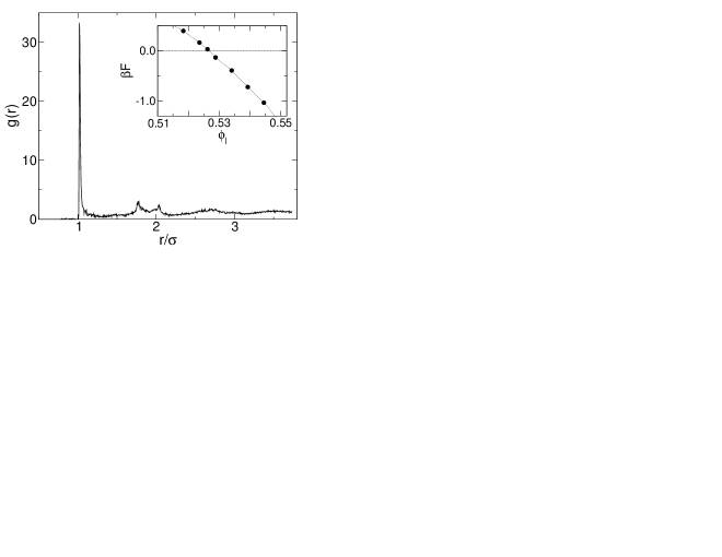
Figure 1: The pair distribution function $g(r)$ of a glassy minimum at $\phi_{l}=0.526$ obtained using the Gaussian superposition approximation and the HG form of $C(r)$. The inset shows the variation of the dimensionless free energy (${\beta}F$) of the glassy minimum with the reference liquid packing fraction $\phi_{l}$.

In order to measure the widths of the local peaks of the density field at a glassy minimum, we have evaluated the quantities $\langle{\delta}r\rangle_{i}=(\int_{v_{i}}d{\bf r}\,|{\bf r}-{\bf R}_{i}|^{2}\rho({\bf r}))^{\frac{1}{2}}$, where $v_{i}$ is a small volume centered at the point ${\bf R}_{i}$ (position of the $i$th local peak), such that $\int_{v_{i}}d{\bf r}\,\rho({\bf r})=1$. We find that, indeed, the values of $\langle{\delta}r\rangle_{i}$ are widely distributed, as can be seen from Fig.2, where we have plotted the distribution of $\langle{\delta}r\rangle$, scaled by its spatial average $\langle{\delta}r\rangle_{\hbox{av}}$, for a glassy minimum at $\phi_{l}=0.55$. The distribution in Fig. 2 is qualitatively similar to those of the dynamical propensity and the local Debye-Waller factor obtained in simulations harrowell1 ; harrowell ; volm .

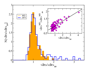
Figure 2: Distribution of $\langle{\delta}r\rangle$, scaled by its average value, for a glassy minimum at $\phi_{l}=0.55$ obtained using the Gaussian approximation and the HG $C(r)$. The distribution of the rms displacement $\langle\delta r\rangle^{\hbox{MD}}$ obtained from MD simulations is also shown for comparison. Inset: correlation between $\langle\delta r\rangle^{\hbox{MD}}$ and $\langle\delta r\rangle$ (the straight line is a guide to the eye).

To make a direct comparison between these DFT results and the dynamics of the system, we have performed MD simulations of the dynamics of the system near a free energy minimum. In these simulations, the values of $\{{\bf R}_{i}\}$ obtained in the free-energy minimization are taken to be the initial particle positions. A few occurrences of neighboring local density peaks separated by less than $\sigma$ are removed using a local relaxation procedure relax . Starting from the same initial configuration but using different sets of initial velocities randomly assigned from the Maxwell-Boltzmann distribution, we have simulated the dynamics for $10^{5}$ collisions per particle, which corresponds to the middle of the plateau of the mean-square displacement of the particles from their initial positions. Using $100$ such different trajectories, we have calculated the rms displacements, $\{\langle\delta r\rangle_{i}^{\hbox{MD}}\}$, of all the particles from their average positions. As shown in Fig. 2, the distribution of $\langle\delta r\rangle^{\hbox{MD}}$ scaled by its average over all the particles is nearly identical to the distribution of $\langle\delta r\rangle$ obtained in the DFT calculation.

To test whether particles that have (small) large values of $\langle\delta r\rangle$ in the DFT calculation show (small) large values of the rms displacement in the MD simulation, we have performed free-energy minimizations starting from 15 particle configurations obtained in the MD simulation. To account for small differences between the initial particle positions and the positions of the local density peaks at the corresponding free-energy minimum, we have divided the system into 125 “cells” of equal volume and averaged both the DFT and MD values of $\langle\delta r\rangle$ over the particles lying in each cell. The inset of Fig. 2 illustrates the correlation between these spatially “coarse-grained” values of $\langle\delta r\rangle$ obtained from DFT and MD calculations. The degree of correlation is quite large, with a correlation coefficient of about 0.76. The correlation coefficient is larger ($\simeq 0.85$) for the subset consisting of 10% of data points with the highest values of $\langle\delta r\rangle/\langle\delta r\rangle_{\hbox{av}}$.

Next, we have removed the Gaussian constraint on the density field and obtained glassy free-energy minima using a numerical schemecdotv for minimizing a discretized version of the RY functional for hard spheres. To discretize the RY functional, a simple cubic computational mesh of size $L^{3}$ and with periodic boundary conditions is introduced. On the sites of this mesh, we define density variables $\rho_{i}\equiv\rho({\bf r}_{i})h^{3}$, where $\rho({\bf r}_{i})$ is the density at site $i$ and $h$ the spacing of the computational mesh. The free energy of Eq.(1) is then numerically minimized as a function of the density variables cdotv .

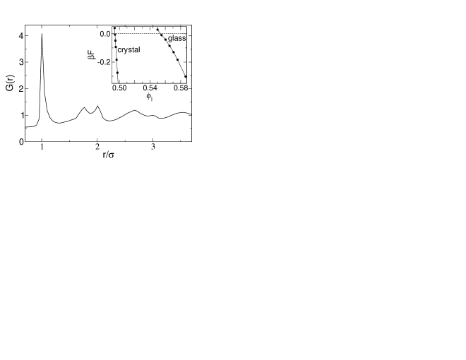
Figure 3: The correlation function $G(r)$ of the time-averaged local density for a glassy minimum at $\phi_{l}=0.586$, obtained from unconstrained minimization using the PY $C(r)$. The inset shows the variation of the free energy of the glassy minimum and that of the fcc crystal with the packing fraction $\phi_{l}$.

In the numerical minimization, we use the Percus-Yevick (PY) expression for ${C(r)}$percus because it leads to (see below) a very accurate value of the crystallization density. The input density field $\{\rho_{i}\}$ for the minimization is obtained using configurations from a MD simulation, for a mesh-spacing $h\simeq 0.05{{\sigma}}$. From the minimization of the free energy as a function of $4.096\times 10^{6}$ density variables, we have again obtained local minima with glassy $\{\rho_{i}\}$. The structure of a local minimum can be characterized by the two-point correlation function $G(r)$ of the time-averaged local density variables $\rho_{i}$ at the minimum (this function is different from the pair distribution function $g(r)$ of Fig. 1). In Fig.3, we have plotted the $G(r)$ for a glassy free-energy minimum at $\phi_{l}=0.586$. The glassy nature of the density distribution is indicated by the split second peak of $G(r)$ and the positions of the two sub-peaks john . The inset of Fig.3 shows the variation of the free energy with the packing fraction $\phi_{l}$, which indicates that the free energy of the glassy minimum crosses that of the liquid at $\phi_{l}=0.554$ which is very close to the packing fraction at the ideal glass transition of mode-coupling theory. Also shown in the plot is the free energy of the fcc crystalline minimum, which becomes negative at $\phi_{l}\simeq 0.497$, a value very close to the known packing fraction at crystallization.

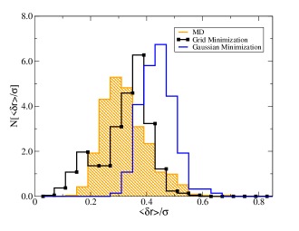
Figure 4: Distribution of $\langle{\delta}r\rangle$ at a glassy minimum obtained using unconstrained minimization with the PY $C(r)$ for $\phi_{l}=0.613$. The distribution of the same quantity obtained using the Gaussian approximation with the same $C(r)$ and the distribution of $\langle\delta r\rangle^{\hbox{MD}}$ obtained from MD simulations are also shown for comparison.

Using the values of $\{\rho_{i}\}$ at a glassy minimum, we have identified the local density peaks and calculated their widths $\{\langle{\delta}r\rangle_{i}\}$, as in the calculation using the Gaussian approximation. It is clear from Fig.4, which shows the distribution of $\langle{\delta}r\rangle$ for a minimum at $\phi_{l}=0.613$, that glassy minima obtained using this scheme also exhibit considerable spatial heterogeneity in the values of $\langle{\delta}r\rangle$. To relate these results to the dynamics, we have performed MD simulations, as described above, starting from the particle configuration obtained from a free-energy minimum found in the unconstrained minimization. These runs consist of 50 different trajectories, each for $10^{5}$ collisions per particle. As shown in Fig. 4, the distribution of the rms displacements obtained from these MD runs is quite similar to the distribution of $\langle\delta r\rangle$ obtained in the DFT calculation. The means and standard deviations of the two distributions, $0.35\sigma$ and $0.08\sigma$, respectively, from MD and $0.34\sigma$ and $0.09\sigma$ from DFT, are nearly the same. Typical values of $\langle\delta r\rangle_{i}$ obtained using the HG $C(r)$ are about three times smaller than those shown in Fig. 4. Similar unrealistically small values of the peak widths were obtained in earlier DFT calculations  das ; kim using the HG $C(r)$. We expect the results obtained using the PY $C(r)$ to be more reliable.

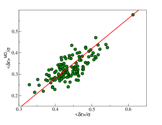
Figure 5: Correlation of the $\langle{\delta}r\rangle$ for a glassy minimum at $\phi_{l}=0.613$ (obtained using the Gaussian approximation with the PY $C(r)$, see text) with the rms displacement $\langle{\delta}r\rangle^{\hbox{MD}}$ obtained from MD simulations. The straight line is a guide to the eye.

Since the local density peaks at the free-energy minimum obtained using the PY $C(r)$ are much broader, the process of elimination of neighboring peaks separated by less than $\sigma$ causes substantial rearrangement of the particles. For this reason, a particle-by-particle comparison of these DFT results with the corresponding MD results is not possible. To make such a comparison, we have done a new calculation using the Gaussian approximation, but this time with the PY $C(r)$, to locate a free-energy minimum in which the local density peaks coincide with the particle positions in the initial configuration used in the MD runs. In this calculation, the density profile is assumed to have the form of Eq.(2) and the free energy is minimized with respect to the parameters $\{\alpha_{i}\}$ and $\{\eta_{i}\}$, keeping $\{{\bf R}_{i}\}$ fixed. Fig. 5 shows the correlation between the $\{\langle\delta r\rangle_{i}\}$ obtained from this DFT calculation and the $\{\langle\delta r\rangle_{i}^{\hbox{MD}}\}$ obtained from MD simulations (both spatially “coarse-grained” using 125 cells as before). This plot shows a high degree of correlation, with a correlation coefficient of 0.75 (it increases to 0.87 for 10% of data points with the highest values of $\langle\delta r\rangle$). Also, as shown in Fig.4, the distribution of $\langle\delta r\rangle$ obtained from this Gaussian DFT calculation is similar to those obtained from the other calculations. These results and those shown in Fig. 2 establish a direct connection between dynamical heterogeneity and the structure of glassy free-energy minima by showing that if a small region of a free-energy minimum contains local density peaks with small (large) widths, then the particles in the same region are very likely to exhibit small (large) values of rms displacement for dynamics near this minimum.

To summarize, using DFT, we have shown that at a glassy minimum of the free-energy of the hard-sphere system, the degree of localization of the local particle density exhibits large spatial variation. Also, by carrying out MD simulations starting from a particle configuration corresponding to the density distribution at a glassy minimum, we have established that the time-averaged density distribution at the minimum is closely related to the dynamical heterogeneity exhibited by the system.

We are grateful to Robin Speedy for useful discussions and Dhrubaditya Mitra for help in computation. PC would like to thank SERC (IISc) for computation facilities and JNCASR for financial support.

References

- (1) M.D. Ediger, Annu. Rev. Phys. Chem. 51, 99 (2000).
- (2) D. N. Perera and P. Harrowell, Phys. Rev. Lett. 81, 120 (1998); W. Kob, C. Donati, S. Plimpton, P.H. Poole and S.C. Glotzer, Phys. Rev. Lett. 79, 2827 (1997).
- (3) A. Widmer-Cooper and P. Harrowell, Phys. Rev. Lett. 93, 135701 (2004).
- (4) A. Widmer-Cooper, P. Harrowell and H. Fynewever, Phys. Rev. Lett 96, 185701 (2006).
- (5) G.A. Appignanesi, J.A. Rodriguez-Fris and M.A. Frechero, Phys. Rev. Lett. 96, 237803 (2006).
- (6) K. Vollmayr-Lee and A. Zippelius, Phys. Rev. E 72, 041507 (2005).
- (7) X. Xia and P.G. Wolynes, Phys. Rev. Lett. 86, 5526 (2001).
- (8) C. Dasgupta and O.T. Valls Phys. Rev. E 53 2603 (1996); ibid. 59, 3123 (1999).
- (9) M. Mezard and G. Parisi, J. Phys. Condens. Mat. 12, 6655 (2000).
- (10) T.V. Ramakrishnan and M. Yussouff, Phys. Rev. B 19, 2775 (1979).
- (11) G. Biroli and J.-P. Bouchaud, Europhys. Lett. 67, 21 (2004).
- (12) Y. Singh, J.P. Stoessel and P.G. Wolynes, Phys. Rev. Lett. 54, 1059 (1985).
- (13) C. Kaur and S.P. Das, Phys. Rev. Lett. 86, 2062 (2001).
- (14) K. Kim and T. Munakata, Phys. Rev. E 68, 021502 (2003).
- (15) D. Henderson and E. W. Grundke, J. Chem. Phys. 63, 601 (1975).
- (16) A.S. Clarke and H. Jonsson, Phys. Rev. E 47, 3975 (1993).
- (17) C.S. O’Hern, S.A. Langer, A.J. Liu and S.R. Nagel, Phys. Rev. Lett. 88, 75507 (2002).
- (18) J.K. Percus and G.J. Yevick, Phys. Rev.110, 1 (1958).