Algebraic fidelity decay for local perturbations

Abstract

From a reflection measurement in a rectangular microwave billiard with randomly distributed scatterers the scattering and the ordinary fidelity was studied. The position of one of the scatterers is the perturbation parameter. Such perturbations can be considered as local since wave functions are influenced only locally, in contrast to, e. g., the situation where the fidelity decay is caused by the shift of one billiard wall. Using the random-plane-wave conjecture, an analytic expression for the fidelity decay due to the shift of one scatterer has been obtained, yielding an algebraic $1/t$ decay for long times. A perfect agreement between experiment and theory has been found, including a predicted scaling behavior concerning the dependence of the fidelity decay on the shift distance. The only free parameter has been determined independently from the variance of the level velocities.

A versatile tool to describe the quantum mechanical stability of a system against perturbations is fidelity introduced by Peres 25 years ago Peres (1984). The fidelity amplitude is defined as the overlap integral of an initial state $|\psi_{0}\rangle$ with itself, after having experienced two slightly different time evolutions,

$$f(t)=\langle\psi_{0}|e^{2\pi\imath H_{0}t}e^{-2\pi\imath H_{1}t}|\psi_{0}\rangle.$$ (1)

Here $H_{0}$ and $H_{1}=H_{0}+\lambda V$ are the two relevant Hamiltonians, and parameter $\lambda$ describes the strength of the perturbation. Throughout this letter the time will be given in units of the Heisenberg time $t_{H}=\hbar/\Delta E$, where $\Delta E$ is the mean level spacing. The fidelity $F(t)$ is the modulus square of the fidelity amplitude. The concept of fidelity is closely related to the concept of decoherence which is widely used in the community of quantum computation Karkuszewski et al. (2002); Gorin et al. (2004a).

For very weak perturbation strengths $\lambda$, in the perturbative regime, Eq. (1) reduces to

$$f(t)=\langle\psi_{0}|e^{-2\pi\imath\lambda V_{\rm diag}t}|\psi_{0}\rangle\,,$$ (2)

where $V_{\rm diag}$ is the diagonal part of the perturbation in the basis of $H_{0}$. Assuming a Gaussian distribution for the matrix elements of $V_{\rm diag}$ Eq. (2) describes a Gaussian decay of the fidelity beyond the Heisenberg time. With increasing perturbation strength the Gaussian decay is taken over by an exponential decay below the Heisenberg time with a decay constant which can be calculated from the matrix elements of the perturbation by means of Fermi’s golden rule Jalabert and Pastawski (2001); Jacquod et al. (2001); Cerruti and Tomsovic (2002). For perturbations with missing diagonals the Gaussian decay is suppressed leaving only the exponential decay, a situation termed freeze Prosen and Žnidarič (2005). For very strong perturbation strengths the fidelity decay becomes independent on the perturbation strength and reflects the classical dynamics. In chaotic systems an exponential decay with the classical Lyapunov exponent is observed Cucchietti et al. (2002), whereas in integrable and diffusive systems an algebraic tail is found Jacquod et al. (2003); Adamov et al. (2003). For more details it is referred to the review article by Gorin et al Gorin et al. (2006a).

In all references mentioned above global perturbations have been considered, meaning that there is a total rearrangement of spectrum and eigenfunctions already for moderate perturbation strengths. For this situation random matrix theory, assuming uncorrelated Gaussian distributions for the matrix elements of $V$, has yielded a number of perturbative and exact results Gorin et al. (2004b); Stöckmann and Schäfer (2005). The fidelity decay by global perturbations has been studied experimentally in a microwave billiard, where one wall was shifted Schäfer et al. (2005), and in a vibrating aluminum block, where the temperature took the role of the perturbation parameter Lobkis and Weaver (2003); Gorin et al. (2006b). In chaotic systems the long time fidelity for global perturbation always is either Gaussian or single exponential, a very unsatisfactory situation, e. g., for quantum computing.

The role of local perturbations, realized in billiard systems, e. g., by the shift of an impurity, has been more or less ignored in the past. This is somewhat surprising, since many, if not most of the perturbing interactions in real systems are short ranged. Examples are diffusive jumps or flips of neighbored spins in solids leading to the decay of spin echoes in nuclear magnetic resonance (see e. g. Ref. Slichter (1980)). Another example is the twinkling of stars, caused by the diffusive motion of the atoms in the atmosphere.

In a previous work we studied the spectral level dynamics in microwave billiards for global variations, realized by a shift of one wall, and local variations, realized by the shift of an impurity Barth et al. (1999). For global variations a Gaussian eigenvalue velocity distribution was found, as expected for chaotic systems. For local perturbations the situation was found to be completely different. The introduction of a point-like impurity leads to a shift of the eigenvalues by

$$\Delta E_{n}=\alpha|\psi_{n}(r)|^{2}\,,$$ (3)

where $\alpha$ describes the strength of the perturbation, and $\psi_{n}$ is the wave function at the scatterer position in the absence of the scatterer. Using the random-plane-wave assumption a modified Bessel function was obtained for the velocity distribution. With increasing radius of the impurity or, equivalently, with increasing frequency a gradual transition from local to global behavior was found. Somewhat later our results had been verified in supersymmetry calculations Marchetti et al. (2003).

In view of the fact that the velocity distributions for global and local perturbations are completely different one could expect that the same is true for the fidelity decay. It will be shown in this letter that this is really the case. We shall see that for local perturbations the fidelity decays algebraically for long times, i. e. the situation is much more favorable than it is the case for global perturbations.

The fidelity in its original definition (1) is hardly accessible experimentally. This was our motivation in a previous work Schäfer et al. (2005) to introduce the scattering fidelity being defined as

$$f^{\mathrm{scat}}(t)=\frac{\displaystyle\hat{C}[S_{ab},S_{ab}^{(\lambda)\ast}](t)}{\displaystyle\sqrt{\hat{C}[S_{ab},S_{ab}^{\ast}](t)\cdot\hat{C}[S_{ab}^{(\lambda)},S_{ab}^{(\lambda)\ast}](t)}}\,.$$ (4)

Here $S_{ab}$ is a scattering matrix element, and $\hat{C}[S_{ab},S_{ab}^{(\lambda)\ast}](t)$ the Fourier transform of the cross-correlation function of the respective matrix elements. It was stated in Ref. Schäfer et al. (2005), that for chaotic systems and weak coupling of the measuring antenna the scattering fidelity approaches the ordinary fidelity. In the present work it has been possible to study both quantities at the same time and to compare the results. Since in all previous experiments on fidelities actually scattering fidelities or related quantities had been measured, though without stating this explicitly, such a comparison is of fundamental interest.

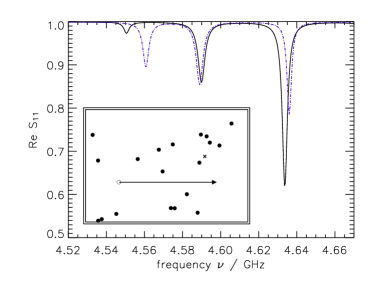
Figure 1: Part of the reflection spectrum for two perturber positions differing by $|\Delta r|=4\,\mathrm{mm}$. The inset shows a sketch of the used microwave billiard (scatterers are shown three times larger). The antenna position is marked by a cross.

The system studied was a rectangular microwave billiard with height $h=8\,\mathrm{mm}$, side lengths $a=340\,\mathrm{mm}$, $b=240\,\mathrm{mm}$ and 19 disks with a diameter of $D=4.6\,\mathrm{mm}$ placed randomly inside the billiard (see inset of Fig. 1). Another disk of the same size has been moved in steps of $|\Delta r|=1\,\mathrm{mm}$ through the billiard. With a fixed wire antenna we measured the reflection spectrum for 300 different positions of the moving disk in a frequency range from 3.5 GHz to 6 GHz. In this frequency range the billiard can still be treated as two-dimensionally, and there is a complete agreement with the corresponding quantum mechanical system Stöckmann (1999). Figure 1 shows part of the reflection spectrum for two slightly different positions of the movable disk. In addition we measured the eigenfunctions Stein and Stöckmann (1992) to make sure that they are delocalized and their intensities Porter-Thomas distributed. Thus the system is fully chaotic and ballistic in the investigated frequency range. In the measured frequency regime it was also possible to extract resonance positions and amplitudes from the spectrum by a Lorentz fit. These quantities will be needed later for the determination of the ordinary fidelity.

First we shall derive an explicit expression of the fidelity decay caused by the shift of a local perturber. We assume that the system is completely chaotic (in the experiment this was verified by measuring the eigenfunctions, see above). In this case we may average expression (1) over all possible initial states resulting in

$$f(t)=\frac{1}{N}{\rm Tr}\left(e^{2\pi\imath H_{0}t}e^{-2\pi\imath H_{1}t}\right)\,,$$ (5)

where $N$ is the number of states taken in the trace. In the present case $H_{0}$ and $H_{1}$ correspond to the Hamiltonian of the billiard with the perturber placed at two different positions. For a weak, point-like perturbation, the perturber just produces a small shift of the eigenenergy proportional to the intensity $|\psi|^{2}$ of the unperturbed wave function at the perturber position, see Eq. (3), i. e. the Hamiltonian in the basis of the unperturbed system is given by

$$H_{nm}(r)=\delta_{nm}(E_{n}^{0}+\alpha|\psi_{n}(r)|^{2})\,,$$ (6)

where the $E_{n}^{0}$ are the eigenenergies of the unperturbed system. For this approach to be valid it is essential that the shift induced by the perturber is always small compared to the mean level spacing, i. e. we never leave the perturbative regime. We then obtain from Eqs. (2) and (6)

$$f(t)=\left\langle e^{2\pi\imath\alpha(|\psi_{1}|^{2}-|\psi_{2}|^{2})}\right\rangle\,,$$ (7)

where the abbreviation $\psi_{i}=\psi(r_{i})$ has been used. The brackets denotes the average over all $N$ participating states. To calculate this average, we now apply the random plane wave assumption. The average is most conveniently expressed in the following way Srednicki and Stiernelof (1996),

$$f(t) = \frac{\sqrt{|K|}}{2\pi}\int\!\!\int d\psi_{1}d\psi_{2}e^{2\pi\imath\alpha(|\psi_{1}|^{2}-|\psi_{2}|^{2})}$$ (8)

$$\qquad\qquad\quad\times e^{-\frac{1}{2}(\psi_{1},\psi_{2})K(\psi_{1},\psi_{2})^{T}}\,,$$

where $K$ is a $(2\times 2)$-matrix of which the inverse

$$K^{-1}=\left(\begin{aligned} \langle\psi_{1}\psi_{1}\rangle&\quad&\langle\psi_{1}\psi_{2}\rangle\\ \langle\psi_{2}\psi_{1}\rangle&\quad&\langle\psi_{2}\psi_{2}\rangle\\ \end{aligned}\right)$$ (9)

can be expressed in terms of two-point correlation functions only. Using again the model of random plane waves Berry (1977) the two-point correlation function can be calculated yielding $\langle\psi_{i}\psi_{j}\rangle=\frac{1}{A}J_{0}(k|r_{i}-r_{j}|)$, where $A$ is the billiard area. Performing the integrations one obtains the final expression for the fidelity amplitude

$$f(t)=\left[1+(\lambda t)^{2}\right]^{-\frac{1}{2}}\,,$$ (10)

where

$$\lambda=\frac{4\pi\alpha}{A}\sqrt{1-J^{2}_{0}(k|\Delta r|)}\,.$$ (11)

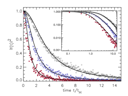
Figure 2: Scattering fidelity (color online) for different shifts of the perturber $|\Delta r|=1$ mm (open circles, black), 2 mm (crosses, blue), and 4 mm (filled squares, red). The solid line corresponds to the theoretical prediction of Eq. (10). The results were obtained for the frequency range from 3.5 GHz to 6 GHz. The insert shows the same results in a double-logarithmic plot.

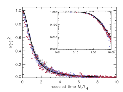
Figure 3: Same as Fig. 2, but plotted on a rescaled time axis using the scaling property of Eq. (10).

$|\Delta r|$ is the shift of the scatterer. For large $t$ the fidelity amplitude decays algebraically with $f(t)\sim 1/t$. The only free parameter in Eq. (11) is $\alpha$. This parameter can be obtained independently from the variance of the level velocities (see Ref. Cerruti and Tomsovic, 2002). This allows us to compare the experimental results with theory without any free parameter.

Figure 2 shows the scattering fidelity, as obtained from Eq. (4), for three different perturber shifts. The solid lines correspond to the theoretical prediction from Eq. (10). A good agreement between theory and experiment is found in all cases, apart from minor systematic deviations for small times. Values obtained for the coupling parameter $\alpha$ by a fit deviate from those from the level velocities by a few %. The inset shows the results in a double-logarithmic plot illustrating the algebraic decay for long times $t$. Equation (10) exhibits a scaling behavior: On a rescaled time axis $\lambda t$ all experimental results should fall onto one single curve. Figure 3 demonstrates that this is indeed the case.

So far we have discussed the results for the scattering fidelity. Let us now see, how the ordinary fidelity (1) can be obtained. Since the measurement has been performed at a fixed antenna position $r_{0}$, the initial state is localized at $r_{0}$, i. e. $|\psi_{0}\rangle=|r_{0}\rangle=\delta(r-r_{0})$. Expanding $|\psi_{0}\rangle$ in terms of eigenfunctions $|\psi_{n}^{1}\rangle$ of $H_{1}$, and $\langle\psi_{0}|$ in terms of eigenfunctions $\langle\psi_{n}^{0}|$ of $H_{0}$, Eq. (1) reads

$$f(t)=\sum\limits_{n,m}\psi_{n}^{0}(r_{0})\psi_{m}^{1}(r_{0})e^{2\pi\imath\left(E_{n}^{0}-E_{m}^{1}\right)t}\langle\psi_{n}^{0}|\psi_{m}^{1}\rangle\,.$$ (12)

The shift of the energy is a first order effect of the perturber, the change of the eigenfunctions being of the next order. Neglecting these higher order effects, we may approximate $\langle\psi_{n}^{0}|\psi_{m}^{1}\rangle\approx\delta_{nm}$ to obtain

$$f(t)=\sum\limits_{n}\psi_{n}^{0}(r_{0})\psi_{n}^{1}(r_{0})e^{2\pi\imath\left(E_{n}^{0}-E_{n}^{1}\right)t}\,.$$ (13)

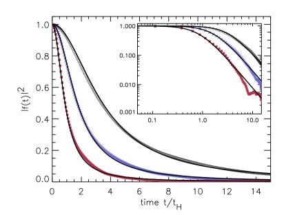
Figure 4: Ordinary fidelity determined as obtained from the resonance position and depths, see text. The meaning of the symbols is the same as in Fig. 2.

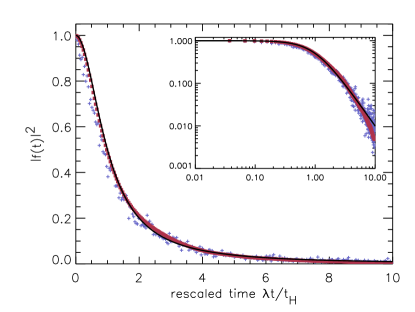
Figure 5: Scattering fidelity, obtained from a superposition of the results from all perturber shifts (blue crosses) and ordinary fidelity (red squares) on a rescaled time axis. The solid line corresponds to the theoretical prediction.

All quantities entering the sum on the right hand side are available from the experiment, the eigenenergies from the resonance positions, and the eigenfunctions at the antenna position from the resonance depths Kuhl et al. (2000). Altogether 64 resonances have been taken. In Fig. 4 the results for the fidelity are presented. A very good agreement between theory and experiment is found. Here the relative deviation for the coupling parameter $\alpha$ taken from the variance of the level velocities and the one obtained from the fidelity even agree up to 1%. No smoothing has been applied. The ordinary fidelity, too, shows the scaling behavior predicted by Eq. (10) as is pronounced in Fig. 5. In addition the collected results for the scattering fidelity, obtained by an averaging over all perturber shifts, is plotted, showing the quality of the agreement between both types of fidelity.

In summary we have shown that for a local perturbation, realized by the shift of a perturber in a microwave billiard, the fidelity decays algebraically with a $1/t$ long-time behavior. This is in contrast to the exponential or Gaussian long-time behavior observed in the fidelity decay due to global perturbations. All results could be quantitatively explained within the random plane wave model, including a scaling prediction on the dependence of the fidelity decay on the perturber shift. In addition we could show that scattering fidelity and ordinary fidelity are identical within the experimental errors.

T. Seligman, Cuernavaca, Mexico, is thanked for numerous discussions and suggestions. This work was founded by the Deutsche Forschungsgemeinschaft via the Forschergruppe 760 “Scattering Systems with Complex Dynamics”.

References

- Peres (1984) A. Peres, Phys. Rev. A 30, 1610 (1984).
- Karkuszewski et al. (2002) Z. P. Karkuszewski, C. Jarzynski, and W. H. Zurek, Phys. Rev. Lett. 89, 170405 (2002).
- Gorin et al. (2004a) T. Gorin, T. Prosen, T. H. Seligman, and W. T. Strunz, Phys. Rev. A 70, 042105 (2004a).
- Jacquod et al. (2001) P. Jacquod, P. G. Silvestrov, and C. W. J. Beenakker, Phys. Rev. E 64, 055203(R) (2001).
- Cerruti and Tomsovic (2002) N. R. Cerruti and S. Tomsovic, Phys. Rev. Lett. 88, 054103 (2002).
- Jalabert and Pastawski (2001) R. A. Jalabert and H. M. Pastawski, Phys. Rev. Lett. 86, 2490 (2001).
- Prosen and Žnidarič (2005) T. Prosen and M. Žnidarič, Phys. Rev. Lett. 94, 044101 (2005).
- Cucchietti et al. (2002) F. M. Cucchietti, C. H. Lewenkopf, E. R. Mucciolo, H. M. Pastawski, and R. O. Vallejos, Phys. Rev. E 65, 046209 (2002).
- Jacquod et al. (2003) P. Jacquod, I. Adagideli, and C. W. J. Beenakker, Europhys. Lett. 61, 729 (2003).
- Adamov et al. (2003) Y. Adamov, I. V. Gornyi, and A. D. Mirlin, Phys. Rev. E 67, 056217 (2003).
- Gorin et al. (2006a) T. Gorin, T. Prosen, T. H. Seligman, and Žnidarič, Phys. Rep. 435, 33 (2006a).
- Gorin et al. (2004b) T. Gorin, T. Prosen, and T. H. Seligman, New J. of Physics 6, 20 (2004b).
- Stöckmann and Schäfer (2005) H.-J. Stöckmann and R. Schäfer, Phys. Rev. Lett. 94, 244101 (2005).
- Schäfer et al. (2005) R. Schäfer, T. Gorin, T. H. Seligman, and H.-J. Stöckmann, New J. of Physics 7, 152 (2005).
- Lobkis and Weaver (2003) O. I. Lobkis and R. L. Weaver, Phys. Rev. Lett. 90, 254302 (2003).
- Gorin et al. (2006b) T. Gorin, T. H. Seligman, and R. L. Weaver, Phys. Rev. E 73, 015202(R) (2006b).
- Slichter (1980) C. P. Slichter, Principles of Magnetic Resonance (Springer, Berlin, 1980).
- Barth et al. (1999) M. Barth, U. Kuhl, and H.-J. Stöckmann, Phys. Rev. Lett. 82, 2026 (1999).
- Marchetti et al. (2003) F. M. Marchetti, I. E. Smolyarenko, and B. D. Simons, Phys. Rev. E 68, 036217 (2003).
- Stöckmann (1999) H.-J. Stöckmann, Quantum Chaos - An Introduction (University Press, Cambridge, 1999).
- Stein and Stöckmann (1992) J. Stein and H.-J. Stöckmann, Phys. Rev. Lett. 68, 2867 (1992).
- Srednicki and Stiernelof (1996) M. Srednicki and F. Stiernelof, J. Phys. A 29, 5817 (1996).
- Berry (1977) M. V. Berry, J. Phys. A 10, 2083 (1977).
- Kuhl et al. (2000) U. Kuhl, E. Persson, M. Barth, and H.-J. Stöckmann, Eur. Phys. J. B 17, 253 (2000).