KA-TP-34-2007

Correlation of energy density
in deconfining SU(2) Yang-Mills thermodynamics

Jochen Keller^†, Ralf Hofmann^∗ and Francesco Giacosa^∗∗

$\mbox{}^{\dagger}$ Institut für Theoretische Physik
Universität Heidelberg
Philosophenweg 16
69120 Heidelberg, Germany

$\mbox{}^{*}$ Institut für Theoretische Physik
Universität Karlsruhe (TH)
Kaiserstr. 12
76131 Karlsruhe, Germany

$\mbox{}^{**}$ Institut für Theoretische Physik
Universität Frankfurt
Max von Laue-Str. 1
60438 Frankfurt, Germany

We compute the two-point correlation of the energy density for the massless mode in deconfining SU(2) Yang-Mills thermodynamics and point towards a possible application for the physics of cold, dilute, and stable clouds of atomic hydrogen within the Milky Way.

1 Introduction

Even at high temperatures the thermodynamics of an SU(2) Yang-Mills theory is interesting judged from both a theoretical and a phenomenological view point.

On the theoretical side, it was argued a long time ago that this system exhibits a magnetic infrared instability when approached in terms of a perturbative expansion [1, 2, 3]. The typical alternating behavior of loop-expanded thermodynamical quantities such as the pressure, which expresses this fact, was impressively demonstrated in thermal perturbation theory [4, 5, 6, 7, 8, 9, 10]. In [11, 12] the concept of a thermal ground state at high temperature was introduced to address the stabilization issue in the magnetic infrared sector. Namely, a spatial coarse-graining over interacting, topologically nontrivial field configurations of charge modulus unity was performed to yield an inert adjoint scalar field and a pure-gauge configuration to describe this ground state. The (temperature dependent) spectrum of excitations after coarse-graining is determined by the adjoint Higgs mechanism. In the according effective theory this tree-level result seems to capture on the one-loop level 99.5% of the contributions to the pressure. The corrections are due to higher loops. It is interesting that the presence of screened and isolated magnetic monopoles [13, 14, 15] in the system is accounted for as a particular radiative correction to the pressure on the two-loop level. That is, on the microsopic level the rare dissociation of calorons or anticalorons, largely deformed away from trivial holonomy, into pairs of massive and screened magnetic monopoles and antimonopoles is seen as a $\propto T^{4}$-correction to the pressure with a small (negative) coefficient after spatial coarse-graining [16]. By cutting the massless line of this two-loop diagram the diagram determining the polarization tensor for this mode is obtained. On shell and depending on the modulus of the spatial momentum the polarization tensor either exhibits screening or antiscreening again thanks to the presence of isolated, screened magnetic monopoles.

The emergence of the thermal ground state implies the dynamical breaking of the SU(2) gauge symmetry down to its U(1) subgroup after spatial coarse-graining [11, 17]. As a consequence, part of the spectrum of the propagating gauge fields acquires a temperature dependent mass thus curing the old problem of a perturbative instability residing in the magnetic sector [1, 2, 3]. Moreover, due to the existence of a dynamically emerging, temperature dependent scale of maximal resolution $|\phi|$ the computation of radiative corrections to the free-quasiparticle situation is under control [17, 19].

On the phenomenological side, radiative corrections in the effective theory can be used to make contact with thermalized photon propagation. To do this the postulate is made that an SU(2) Yang-Mills theory of scale $\sim 10^{-4}\,$eV, referred to as SU(2)${}_{\tiny\mbox{CMB}}$ in the following, underlies the U(1) gauge symmetry of electromagnetism [11, 16, 20]. If verified experimentally through predictions based on radiative effects [21, 22, 23] then cosmological consequences would arise [24]. That is, the nontrivial ground state underlying photon propagation would then be linked to the dynamics of an ultralight and spatially homogeneous scalar field (Planck-scale axion) [25, 26, 27] associated with dark energy. Notice the apparent and amusing paradox: The nonabelian gauge theory underlying the propagation of light would, by means of its ground state, be a crucial ingredient in generating dark energy. Also, there would be immediate implications for the physics of temperature-temperature correlations in the cosmic microwave background (CMB) at large angles [22] and, by virtue of the connection to axion physics, a CP violating electric-magnetic cross correlation (extracted from the according polarization map of the CMB) should be detectable by future satellite missions. There is an alternative physical system for which the radiative effects of SU(2)${}_{\tiny\mbox{CMB}}$ would be relevant: dilute, old, and cold clouds of atomic hydrogen in between the spiral arms of the Milky Way [28].

Notice that these results rely on infinite-volume thermodynamics, that is, on the absence of time-dependent sources and on the requirement that spatial boundaries, imposing additional conditions on the gauge-field dynamics, are well farther apart then the physical correlation lengths of the infinite-volume situation. Away from the phase boundary at $T_{c}\sim 2.7\,$K, where the mass of screened monopoles vanishes and thus the correlation length diverges, the length scale, which separates the infinite-volume case from the boundary case, is set by $|\phi|^{-1}=\frac{(13.87)^{3/2}}{2\pi T_{c}}\,\sqrt{T/T_{c}}$ [11]. Close to $T_{c}$ this is smaller but of the order of one centimeter. For this reason and for the fact that in low-temperature condensed-matter experiments it is not the temperature of a photon gas that is measured it is then clear that the results of the infinite-volume approach do not apply to the conditions prevailing in these systems. In cosmological or astrophysical situations or in a designated black-body experiment with sufficiently large and homogeneously thermalized volume conditions are in line with those assumed when making a prediction for the low-frequency, spectral distortion caused by the scattering of photons off of isolated monopoles [16, 21]. In addition to a black-body experiment for $T\geq T_{c}$ one may also learn about the ground state of SU(2)${}_{\tiny\mbox{CMB}}$ at lower temperatures by detecting the onset of superconductivity in the preconfining phase associated with the condensation of monopoles: Shortly below $T_{c}$ the pressure is larger than the conventional photon-gas pressure due to the emergence of an extra degree of freedom – a longitudinal polarization of the photon, see also [23]. Along the same lines a future precision survey of intergalactic magnetic fields may be able to make quantitative contact with SU(2)${}_{\tiny\mbox{CMB}}$, see [17] for a droplet model describing the statistics of monopole condensing regions.

One may also wonder about whether standard-model (SM) weak-interaction quantum numbers should be assigned to the SU(2)${}_{\tiny\mbox{CMB}}$ gauge fields. The point here is that in light of the underlying gauge symmetry the SM is a (highly successful) effective quantum field theory with quantum numbers and interactions (Higgs sector!) assigned to its effective fields so as to keep the theory consistent (gauge-anomaly cancellation, renormalizability, unitarity). On the level of fundamental gauge fields no such an assignment is needed: The massless mode of SU(2)${}_{\tiny\mbox{CMB}}$ still is the propagating photon $\gamma$ of the SM, and local interactions with electrically charged matter are still described through this gauge field’s mixing with the neutral gauge field of SU(2)_W. In addition, no interactions of the two massive excitations of SU(2)${}_{\tiny\mbox{CMB}}$ with charged or neutral matter and the two massive excitations of SU(2)_W, respectively, takes place due to the existence of a large hierarchy in the participating (Yang-Mills) scales on one hand and the existence of a small compositeness scale $|\phi|$ in SU(2)${}_{\tiny\mbox{CMB}}$ on the other hand, for a more detailed discussion see [24].

The purpose of the present work is to compute the two-point correlation of the canonical energy density $\Theta_{00}$ of photons in a thermalized gas. In the framework of SU(2)${}_{\tiny\mbox{CMB}}$ the canonical energy density of the photon gas (massless modes in unitary gauge, see [11, 16, 29]) is made manifestly SU(2) gauge invariant in the effective theory for deconfining thermodynamics by substituting the ’t Hooft tensor [30] into the expression for the U(1) Belinfante energy-momentum tensor $\Theta_{\mu\nu}$. Recall, that in unitary gauge the ’t Hooft tensor reduces to the abelian field strength for the (massless) mode pointing into the direction of the Higgs field in the algebra. Apart from phenomenological considerations, to compute $\left\langle\Theta_{00}({\bf x})\Theta_{00}({\bf y})\right\rangle$ is technically interesting by itself. Namely, this quantity appears to be accurately calculable in terms of the one-loop photon polarization tensor only. That is, irreducible diagrams beyond two loop appear to yield a safely negligible contribution to $\gamma$’s polarization tensor, compare with the results in [18]. In this work we present results in a minimal way technically to warrant a reasonably efficient flow of the arguments. For calculational details we refer the reader to [31].

The paper is organized as follows. In Sec. 2 we define the problem in a real-time formulation of a thermalized (free) U(1) gauge theory. Thermal and quantum parts of the correlator $\langle\Theta_{00}({\bf x})\Theta_{00}({\bf y})\rangle$ are calculated analytically and compared with one another. The same program is performed for the case of deconfining SU(2) Yang-Mills theory in Sec. 3. Only an estimate is possible analytically for the vacuum contribution, and the thermal part is evaluated numerically. We compare our results to those obtained for the U(1) case and observe a sizable suppression of the SU(2) correlation at low temperatures and large distances. In Sec. 4 we offer a potential explanation of why cold and dilute clouds of atomic hydrogen within the Milky Way are apparently so stable. There is a short summary in Sec. 5.

2 Two-point correlation of energy density in thermal U(1) gauge theory

In this section we compute the two-point correlation of the canonical energy density in a pure, thermalized U(1) gauge theory. Our results will serve as a benchmark for the more involved calculation when embedding this object into a deconfining SU(2) Yang-Mills theory.

2.1 General strategy

The two-point correlation of the energy density is computed by letting derivative operators, associated with the structure of the energy-momentum tensor $\Theta_{\mu\nu}$, act on the real-time propagator of the U(1) gauge field.

Recall that the traceless and symmetric (Belinfante) energy-momentum tensor of a pure U(1) gauge theory is given as

$$\Theta_{\mu\nu}=-F_{\mu}\!^{\lambda}F_{\nu\lambda}+\frac{1}{4}g_{\mu\nu}F^{\kappa\lambda}F_{\kappa\lambda}\,,$$ (1)

where $F_{\mu\nu}\equiv\partial_{\mu}A_{\nu}-\partial_{\nu}A_{\mu}$, and $A_{\mu}$ denotes the U(1) gauge field. In the deconfining phase of SU(2) Yang-Mills thermodynamics the effective theory contains an inert, adjoint Higgs field $\phi$ [11, 17]. The field $\phi$ emerges by a spatial coarse-graining process over topologically nontrivial field configurations of trivial holonomy: Harrington-Shepard calorons and anticalorons [32]. These nonpropagating, BPS saturated, periodic solutions to the euclidean Yang-Mills equations are deformed by gluon exchanges leading to short-lived nontrivial holonomy and thus short-lived, separated magnetic charges [33, 34, 35, 36, 37, 38, 39]. This situation is described by a pure-gauge configuration in the effective theory.

After spatial coarse-graining and owing to the presence of the field $\phi$, the field strength $F_{\mu\nu}$ of the abelian theory in Eq. (1) can be replaced by the ’t Hooft tensor ${\cal F}_{\mu\nu}$ to define an SU(2) gauge invariant energy-momentum tensor. One has [30]

$${\cal F}_{\mu\nu}\equiv\frac{1}{|\phi|}\phi_{a}G_{\mu\nu}^{a}-\frac{1}{e|\phi|^{3}}\epsilon^{abc}\phi_{a}(D_{\mu}\phi)_{b}(D_{\nu}\phi)_{c}\,,$$ (2)

where $G^{a}_{\mu\nu}$ is the SU(2) field strength of topologically trivial, coarse-grained fluctuations, $D_{\mu}$ denotes the adjoint covariant derivative, and $e$ is the effective gauge coupling. Obviously, the quantity defined by the right-hand side of Eq. (2) is SU(2) gauge invariant. In unitary gauge $\phi_{a}=\delta_{a3}|\phi|$ the ’t Hooft tensor reduces to the abelian tensor $F_{\mu\nu}$ defined on the massless gauge field $A_{\mu}^{3}$.

We are interested in computing the connected correlation function $\left\langle\Theta_{00}(x)\Theta_{00}(y)\right\rangle$ in four-dimensional Minkowskian spacetime ($g_{00}=1$). This is done by applying Wick’s theorem to express $\left\langle\Theta_{00}(x)\Theta_{00}(y)\right\rangle$ in terms of the propagator $D_{\mu\nu}$, which in Coulomb gauge and momentum space is given as

$$D_{\mu\nu}(p,T) = D^{\tiny\mbox{vac}}_{\mu\nu}(p,T)+D^{\tiny\mbox{th}}_{\mu\nu}(p,T)$$ (3)

$$= -P^{T}_{\mu\nu}(p)\frac{i}{p^{2}+i\epsilon}+i\frac{u_{\mu}u_{\nu}}{{\bf p}^{2}}-P^{T}_{\mu\nu}(p)2\pi\delta(p^{2})n_{B}(\beta|p_{0}|)\,,$$

where $u_{\mu}=(1,0,0,0)$, $\beta\equiv\frac{1}{T}$,

$$P^{T}_{00}(p) \equiv P^{T}_{0i}(p)=P^{T}_{i0}(p)=0,$$

$$P^{T}_{ij}(p) \equiv \delta_{ij}-\frac{p_{i}p_{j}}{{\bf p}^{2}}\,,$$ (4)

and $n_{B}(x)\equiv\frac{1}{e^{x}-1}$. By virtue of Eq. (1) one obtains

$$\langle\Theta_{00}(x)\Theta_{00}(y)\rangle = 2\langle\partial_{x^{0}}A^{\lambda}(x)\partial_{y^{0}}A^{\tau}(y)\rangle\langle\partial_{x^{0}}A_{\lambda}(x)\partial_{y^{0}}A_{\tau}(y)\rangle$$

$$-g_{00}\langle\partial_{x^{0}}A^{\lambda}(x)\partial_{y^{\sigma}}A^{\tau}(y)\rangle\langle\partial_{x^{0}}A_{\lambda}(x)\partial_{y_{\sigma}}A_{\tau}(y)\rangle$$

$$+g_{00}\langle\partial_{x^{0}}A^{\lambda}(x)\partial_{y_{\sigma}}A^{\tau}(y)\rangle\langle\partial_{x^{0}}A_{\lambda}(x)\partial_{y^{\tau}}A_{\sigma}(y)\rangle$$

$$-g_{00}\langle\partial_{x_{\kappa}}A^{\lambda}(x)\partial_{y^{0}}A^{\tau}(y)\rangle\langle\partial_{x^{\kappa}}A_{\lambda}(x)\partial_{y^{0}}A_{\tau}(y)\rangle$$

$$+g_{00}\langle\partial_{x_{\kappa}}A^{\lambda}(x)\partial_{y^{0}}A^{\tau}(y)\rangle\langle\partial_{x^{\lambda}}A_{\kappa}(x)\partial_{y^{0}}A_{\tau}(y)\rangle$$

$$+\frac{g_{00}^{2}}{2}\langle\partial_{x_{\kappa}}A^{\lambda}(x)\partial_{y_{\sigma}}A^{\tau}(y)\rangle\langle\partial_{x^{\kappa}}A_{\lambda}(x)\partial_{y^{\sigma}}A_{\tau}(y)\rangle$$

$$-\frac{g_{00}^{2}}{2}\langle\partial_{x_{\kappa}}A^{\lambda}(x)\partial_{y_{\sigma}}A^{\tau}(y)\rangle\langle\partial_{x^{\kappa}}A_{\lambda}(x)\partial_{y^{\tau}}A_{\sigma}(y)\rangle$$

$$-\frac{g_{00}^{2}}{2}\langle\partial_{x_{\kappa}}A^{\lambda}(x)\partial_{y_{\sigma}}A^{\tau}(y)\rangle\langle\partial_{x^{\lambda}}A_{\kappa}(x)\partial_{y^{\sigma}}A_{\tau}(y)\rangle$$

$$+\frac{g_{00}^{2}}{2}\langle\partial_{x_{\kappa}}A^{\lambda}(x)\partial_{y_{\tau}}A^{\sigma}(y)\rangle\langle\partial_{x^{\lambda}}A_{\kappa}(x)\partial_{y^{\sigma}}A_{\tau}(y)\rangle$$

$$+2\langle\partial_{x^{0}}A^{0}(x)\partial_{y^{0}}A^{0}(y)\rangle\langle\partial_{x^{0}}A_{0}(x)\partial_{y^{0}}A_{0}(y)\rangle$$

$$-2\langle\partial_{x^{0}}A^{0}(x)\partial_{y^{\tau}}A^{0}(y)\rangle\langle\partial_{x^{0}}A_{0}(x)\partial_{y_{\tau}}A_{0}(y)\rangle$$

$$+2\langle\partial_{x^{\tau}}A^{0}(x)\partial_{y^{\sigma}}A^{0}(y)\rangle\langle\partial_{x_{\tau}}A_{0}(x)\partial_{y_{\sigma}}A_{0}(y)\rangle$$

$$-2g_{00}\langle\partial_{x^{0}}A^{0}(x)\partial_{y^{0}}A^{0}(y)\rangle\langle\partial_{x^{0}}A_{0}(x)\partial_{y^{0}}A_{0}(y)\rangle$$

$$+4g_{00}\langle\partial_{x^{0}}A^{0}(x)\partial_{y^{\tau}}A^{0}(y)\rangle\langle\partial_{x^{0}}A_{0}(x)\partial_{y_{\tau}}A_{0}(y)\rangle$$

$$-2g_{00}\langle\partial_{x^{\tau}}A^{0}(x)\partial_{y^{\sigma}}A^{0}(y)\rangle\langle\partial_{x_{\tau}}A_{0}(x)\partial_{y_{\sigma}}A_{0}(y)\rangle$$

$$+\frac{g_{00}^{2}}{2}\langle\partial_{x^{0}}A^{0}(x)\partial_{y^{0}}A^{0}(y)\rangle\langle\partial_{x^{0}}A_{0}(x)\partial_{y^{0}}A_{0}(y)\rangle$$

$$-g_{00}^{2}\langle\partial_{x^{0}}A^{0}(x)\partial_{y^{\tau}}A^{0}(y)\rangle\langle\partial_{x^{0}}A_{0}(x)\partial_{y_{\tau}}A_{0}(y)\rangle$$

$$+\frac{g_{00}^{2}}{2}\langle\partial_{x^{\tau}}A^{0}(x)\partial_{y^{\sigma}}A^{0}(y)\rangle\langle\partial_{x_{\tau}}A_{0}(x)\partial_{y_{\sigma}}A_{0}(y)\rangle\,.$$

Notice that at this stage ambiguities related to the various possibilities of time ordering in the two-point function of the gauge field $A_{\mu}$ cancel out. The last nine lines in Eq. (2.1) arise from the term $\propto u_{\mu}u_{\nu}$ in the propagator, see Eq. (3).

2.2 Real-time formalism: Decomposition into thermal and vacuum parts

In evaluating the expression in Eq. (2.1) the derivative operators are taken out of the expectation, and Eq. (3) is used. By momentum conservation the expression Eq. (2.1) separates into purely thermal and purely vacuum contributions, see Fig. 1.

Figure 1: Feynman diagram for the correlator $\langle\Theta_{00}(x)\Theta_{00}(y)\rangle$ in a pure U(1) gauge theory. Crosses denote the insertion of the local, composite operator $\Theta_{00}$.

Using

$$P^{T\,\lambda\tau}(p)P^{T}_{\lambda\tau}(k) = 1+\frac{({\bf p}\cdot{\bf k})^{2}}{{\bf p}^{2}{\bf k}^{2}}\,,$$

$$P^{T}_{\lambda\sigma}(p)k^{\lambda}k^{\sigma} = {\bf k}^{2}-\frac{({\bf p}\cdot{\bf k})^{2}}{{\bf p}^{2}}\,,$$

$$P^{T\,\kappa\tau}(p)P^{T}_{\kappa\sigma}(k)p^{\sigma}k_{\tau} = -({\bf p}\cdot{\bf k})\left(\frac{({\bf p}\cdot{\bf k})^{2}}{{\bf p}^{2}{\bf k}^{2}}-1\right)$$ (6)

the purely thermal contribution $\langle\Theta_{00}(x)\Theta_{00}(y)\rangle^{\tiny\mbox{th}}$ (performing the trivial integration over the 0-components of the momenta) reads

$$\langle\Theta_{00}({\bf x})\Theta_{00}({\bf y})\rangle^{\tiny\mbox{th}} = \left(\int\!\!\frac{d^{3}p}{(2\pi)^{3}}|{\bf p}|\,n_{B}(\beta|{\bf p}|)\,\mbox{e}^{i{\bf p}{\bf z}}\right)^{2}$$

$$+ \int\!\!\frac{d^{3}p}{(2\pi)^{3}}\int\!\!\frac{d^{3}k}{(2\pi)^{3}}\left(\frac{{\bf p}{\bf k}}{|{\bf p}||{\bf k}|}\right)^{2}|{\bf p}||{\bf k}|\,n_{B}(\beta|{\bf p}|)n_{B}(\beta|{\bf k}|)\,\mbox{e}^{i{\bf p}{\bf z}}\,\mbox{e}^{i{\bf k}{\bf z}}$$

where ${\bf z}\equiv{\bf x}-{\bf y}$. In deriving Eq. (2.2) we have set $x^{0}=y^{0}$ thus neglecting oscillatory terms. This prescription should reflect the time-averaged energy transport between points ${\bf x}$ and ${\bf y}$ and is technically much easier to handle.

Inserting the vacuum part of the propagator in Eq. (3) into Eq. (2.1), performing similar contractions as in Eq. (2.2), and rotating to euclidean signature ($p_{0},k_{0}\to ip_{0},ik_{0}$, $x^{0},y^{0}\to-ix^{0},-iy^{0}$, $g_{\mu\nu}\to-\delta_{\mu\nu}$), we obtain

$$\langle\Theta_{00}(x)\Theta_{00}(y)\rangle^{\tiny\mbox{vac}}$$

$$=\frac{9}{2}\left(\int\frac{d^{4}p}{(2\pi)^{4}}\,p_{0}^{2}\,\frac{\mbox{e}^{ip\zeta}}{p^{2}}\right)^{2}+\frac{1}{2}\left(\int\frac{d^{4}p}{(2\pi)^{4}}\,|{\bf p}|^{2}\,\frac{\mbox{e}^{ip\zeta}}{p^{2}}\right)^{2}$$

$$+6\int\frac{d^{4}p}{(2\pi)^{4}}\int\frac{d^{4}k}{(2\pi)^{4}}\left(\frac{{\bf p}{\bf k}}{|{\bf p}||{\bf k}|}\right)p_{0}k_{0}|{\bf p}||{\bf k}|\,\frac{\mbox{e}^{ip\zeta}}{p^{2}}\,\frac{\mbox{e}^{ik\zeta}}{k^{2}}$$

$$+\frac{1}{2}\int\frac{d^{4}p}{(2\pi)^{4}}\int\frac{d^{4}k}{(2\pi)^{4}}\left(\frac{{\bf p}{\bf k}}{|{\bf p}||{\bf k}|}\right)^{2}\left(9\,p_{0}^{2}k_{0}^{2}+|{\bf p}|^{2}|{\bf k}|^{2}\right)\,\frac{\mbox{e}^{ip\zeta}}{p^{2}}\,\frac{\mbox{e}^{ik\zeta}}{k^{2}}$$

$$+2\left(\int\frac{d^{4}p}{(2\pi)^{4}}\,p_{0}^{2}\,\frac{\mbox{e}^{ip\zeta}}{{\bf p}^{2}}\right)^{2}$$

$$+2\int\frac{d^{4}p}{(2\pi)^{4}}\int\frac{d^{4}k}{(2\pi)^{4}}\left(\frac{{\bf p}{\bf k}}{|{\bf p}||{\bf k}|}\right)p_{0}k_{0}|{\bf p}||{\bf k}|\frac{\mbox{e}^{ip\zeta}}{{\bf p}^{2}}\,\frac{\mbox{e}^{ik\zeta}}{{\bf k}^{2}}$$

$$+\frac{9}{2}\int\frac{d^{4}p}{(2\pi)^{4}}\int\frac{d^{4}k}{(2\pi)^{4}}\left(\frac{{\bf p}{\bf k}}{|{\bf p}||{\bf k}|}\right)^{2}|{\bf p}|^{2}|{\bf k}|^{2}\,\frac{\mbox{e}^{ip\zeta}}{{\bf p}^{2}}\,\frac{\mbox{e}^{ik\zeta}}{{\bf k}^{2}}\,.$$

where $\zeta\equiv x-y$ and $p\zeta=p_{\mu}\zeta_{\mu},k\zeta=k_{\mu}\zeta_{\mu},p^{2}=p_{\mu}p_{\mu},$ and $k^{2}=k_{\mu}k_{\mu}$. The last three lines in Eq. (2.2) arise from the term $\propto u_{\mu}u_{\nu}$ in the propagator, see Eq. (3).

2.3 Results

To evaluate the integrals in Eqs. (2.2) and (2.2) we introduce rescaled momenta $\tilde{p}_{\mu}\equiv\beta p_{\mu}$ and $\tilde{k}_{\mu}\equiv\beta k_{\mu}$. The integrals in Eqs. (2.2) and (2.2) are now expressed in terms of 3D and 4D spherical coordinates, respectively, and the integration over azimuthal angles is performed in a straight-forward way in both cases. As a result, the integrals over the remaining variables factorize for each term in Eqs.  (2.2) and (2.2).

In case of $\langle\Theta_{00}(\textbf{x})\Theta_{00}(\textbf{y})\rangle^{\tiny\mbox{th}}$ we choose ${\bf z}$ to point into the 3-direction. Making use of the spherical expansion of the exponential

$$e^{i|{\bf\tilde{q}}||{\bf\tilde{{\bf z}}}|\cos\theta}=\sum\limits_{l=0}^{\infty}i^{l}(2l+1)j_{l}(|{\bf\tilde{q}}||{\bf\tilde{{\bf z}}}|)P_{l}(\cos\theta)\,,$$ (9)

where $\theta\equiv\angle({{\bf q},{\bf\zeta}})$, ${\bf\tilde{{\bf z}}}\equiv\frac{{\bf z}}{\beta}$, $q=p,k$, and $j_{l}$ denotes a spherical Bessel function, expressing polynomial factors in $\cos\theta$ in terms of linear combinations of Legendre polynomials $P_{l}(\cos\theta)$, and exploiting their orthonormality relation

$$\int\limits_{-1}^{+1}dx\,P_{n}(x)P_{m}(x)=\frac{2}{2m+1}\delta_{mn}\,,\ \ \ (m,n\ \ \mbox{integer})\,,$$ (10)

in integrating over the polar angle $\theta$, we arrive at

$$\langle\Theta_{00}({\bf x})\Theta_{00}({\bf y})\rangle^{\tiny\mbox{th}} = \frac{1}{(2\pi)^{6}\beta^{8}}\left(\frac{64\pi^{2}}{3}\left(\int\limits_{0}^{\infty}d|\tilde{{\bf p}}|\frac{|\tilde{{\bf p}}|^{3}}{\mbox{e}^{|\tilde{{\bf p}}|}-1}j_{0}(|\tilde{{\bf z}}||\tilde{{\bf p}}|)\right)^{2}\right.$$

$$\left.+\frac{32\pi^{2}}{3}\left(\int\limits_{0}^{\infty}d|\tilde{{\bf p}}|\frac{|\tilde{{\bf p}}|^{3}}{\mbox{e}^{|\tilde{{\bf p}}|}-1}j_{2}(|\tilde{{\bf z}}||\tilde{{\bf p}}|)\right)^{2}\right)$$

Performing the integration over $|\tilde{{\bf p}}|$, we have [40]

$$\langle\Theta_{00}({\bf x})\Theta_{00}({\bf y})\rangle^{\tiny\mbox{th}}=$$

$$\frac{1}{(2\pi)^{6}\beta^{8}}\Bigg{(}\frac{64\pi^{2}}{3}\left(\frac{1}{|\tilde{{\bf z}}|^{4}}-\frac{\pi^{3}\coth(\pi|\tilde{{\bf z}}|)\textrm{cosech}^{2}(\pi|\tilde{{\bf z}}|)}{|\tilde{{\bf z}}|}\right)^{2}$$

$$\left.+\frac{32\pi^{2}}{3}\left(\frac{-8+\pi|\tilde{{\bf z}}|(3\coth(\pi|\tilde{{\bf z}}|)+\pi|\tilde{{\bf z}}|(3+2\pi|\tilde{{\bf z}}|\coth(\pi|\tilde{{\bf z}}|))\,\textrm{cosech}^{2}(\pi|\tilde{{\bf z}}|))}{2|\tilde{{\bf z}}|^{4}}\right)^{2}\right)$$

Figure 2: The ratio $R_{\tiny\mbox{th}-\tiny\mbox{vac};\tiny\mbox{U(1)}}\equiv\frac{\langle\Theta_{00}({\bf x})\Theta_{00}({\bf y})\rangle^{\tiny\mbox{th}}}{\langle\Theta_{00}({\bf x})\Theta_{00}({\bf y})\rangle^{\tiny\mbox{vac}}}$ as a function of $|\tilde{{\bf z}}|$ for a thermalized pure U(1) gauge theory.

In case of $\langle\Theta_{00}(x)\Theta_{00}(y)\rangle^{\tiny\mbox{vac}}$ we restrict to $x_{0}=y_{0}$ to be able to compare with $\langle\Theta_{00}(\textbf{x})\Theta_{00}(\textbf{y})\rangle^{\tiny\mbox{th}}$. Furthermore we chose ${\bf z}$ to point into the 3-direction. We expect $\langle\Theta_{00}(x)\Theta_{00}(y)\rangle^{\tiny\mbox{vac}}$ to be a negligible correction to $\langle\Theta_{00}(\textbf{x})\Theta_{00}(\textbf{y})\rangle^{\tiny\mbox{th}}$ for $|\tilde{{\bf z}}|>1$. In analogy to the thermal case each term in Eq. (2.2) factorizes upon azimuthal integration. Making use of the spherical expansion of the exponential

$$e^{i|{\bf\tilde{q}}||{\bf\tilde{{\bf z}}}|\sin\psi\,\cos\theta}=\sum\limits_{l=0}^{\infty}i^{l}(2l+1)j_{l}(|{\bf\tilde{q}}||{\bf\tilde{{\bf z}}}|\sin\psi)P_{l}(\cos\theta)\,,$$ (13)

where $\psi$ is the second polar angle, expressing polynomial factors in $\cos\theta$ in terms of linear combinations of Legendre polynomials $P_{l}(\cos\theta)$, and exploiting their orthonormality relation (10) in integrating over the first polar angle $\theta$, we arrive at

$$\langle\Theta_{00}({\bf x})\Theta_{00}({\bf y})\rangle^{\tiny\mbox{vac}}=\frac{1}{(2\pi)^{8}\beta^{8}}\left(96\pi^{2}\left(\int\limits_{0}^{\infty}\!\!d|\tilde{p}|\,|\tilde{p}|^{3}\int\limits_{0}^{\pi}\!\!d\psi\,\sin^{2}\psi\cos^{2}\psi j_{0}(|\tilde{p}||\tilde{{\bf z}}|\sin\psi)\right)^{2}\right.$$

$$+\left.48\pi^{2}\left(\int\limits_{0}^{\infty}\!\!d|\tilde{p}|\,|\tilde{p}|^{3}\int\limits_{0}^{\pi}\!\!d\psi\,\sin^{2}\psi\cos^{2}\psi j_{2}(|\tilde{p}||\tilde{{\bf z}}|\sin\psi)\right)^{2}\right.$$

$$+\left.96\pi^{2}\left(\int\limits_{0}^{\infty}\!\!d|\tilde{p}|\,|\tilde{p}|^{3}\int\limits_{0}^{\pi}\!\!d\psi\,\sin^{3}\psi\cos\psi j_{1}(|\tilde{p}||\tilde{{\bf z}}|\sin\psi)\right)^{2}\right.$$

$$+\left.\frac{32\pi^{2}}{3}\left(\int\limits_{0}^{\infty}\!\!d|\tilde{p}|\,|\tilde{p}|^{3}\int\limits_{0}^{\pi}\!\!d\psi\,\sin^{4}\psi j_{0}(|\tilde{p}||\tilde{{\bf z}}|\sin\psi)\right)^{2}\right.$$

$$+\left.\frac{16\pi^{2}}{3}\left(\int\limits_{0}^{\infty}\!\!d|\tilde{p}|\,|\tilde{p}|^{3}\int\limits_{0}^{\pi}\!\!d\psi\,\sin^{4}\psi j_{2}(|\tilde{p}||\tilde{{\bf z}}|\sin\psi)\right)^{2}\right.$$

$$+\left.32\pi^{2}\left(\int\limits_{0}^{\infty}\!\!d|\tilde{p}|\,|\tilde{p}|^{3}\int\limits_{0}^{\pi}\!\!d\psi\,\cos^{2}\psi j_{0}(|\tilde{p}||\tilde{{\bf z}}|\sin\psi)\right)^{2}\right.$$

$$+\left.32\pi^{2}\left(\int\limits_{0}^{\infty}\!\!d|\tilde{p}|\,|\tilde{p}|^{3}\int\limits_{0}^{\pi}\!\!d\psi\,\sin\psi\cos\psi j_{1}(|\tilde{p}||\tilde{{\bf z}}|\sin\psi)\right)^{2}\right.$$

$$+\left.24\pi^{2}\left(\int\limits_{0}^{\infty}\!\!d|\tilde{p}|\,|\tilde{p}|^{3}\int\limits_{0}^{\pi}\!\!d\psi\,\sin^{2}\psi j_{0}(|\tilde{p}||\tilde{{\bf z}}|\sin\psi)\right)^{2}\right.$$

$$+\left.48\pi^{2}\left(\int\limits_{0}^{\infty}\!\!d|\tilde{p}|\,|\tilde{p}|^{3}\int\limits_{0}^{\pi}\!\!d\psi\,\sin^{2}\psi j_{2}(|\tilde{p}||\tilde{{\bf z}}|\sin\psi)\right)^{2}\right)\,,$$

where now $|\tilde{p}|\equiv\sqrt{\tilde{p}_{0}^{2}+\tilde{p}_{1}^{2}+\tilde{p}_{2}^{2}+\tilde{p}_{3}^{2}}$, and $j_{0},j_{1},j_{2}$ are spherical Bessel functions. In Eq. (2.3) the last four lines arise from the term $\propto u_{\mu}u_{\nu}$ in the propagator, see Eq. (3). They vanish because no energy transfer between points ${\bf x}$ and ${\bf y}$ is mediated by the Coulomb part of the photon propagator. Upon performing the integration over $\psi$ the third and seventh line vanish for symmetry reasons. Our final result is

$$\langle\Theta_{00}({\bf x})\Theta_{00}({\bf y})\rangle^{\tiny\mbox{vac}} = \frac{1}{(2\pi)^{8}\beta^{8}}\cdot 96\pi^{2}\cdot\left(\frac{2\pi}{|\tilde{{\bf z}}|^{4}}\right)^{2}+\frac{1}{(2\pi)^{8}\beta^{8}}\cdot 48\pi^{2}\cdot\left(\frac{-8\pi}{|\tilde{{\bf z}}|^{4}}\right)^{2}$$ (15)

$$+\frac{1}{(2\pi)^{8}\beta^{8}}\cdot\frac{32\pi^{2}}{3}\cdot\left(\frac{-2\pi}{|\tilde{{\bf z}}|^{4}}\right)^{2}+\frac{1}{(2\pi)^{8}\beta^{8}}\cdot\frac{16\pi^{2}}{3}\cdot\left(\frac{8\pi}{|\tilde{{\bf z}}|^{4}}\right)^{2}$$

$$= \frac{15}{\pi^{4}\beta^{8}\,|\tilde{{{\bf z}}}|^{8}}=\frac{0.15399}{|{\bf z}|^{8}}\,.$$

We have checked this result by a position-space calculation in Feynman gauge where the vacuum part of the propagator is given as

$$D_{\mu\nu}^{\tiny\mbox{vac}}(x)=\frac{1}{4\pi^{2}x^{2}}g_{\mu\nu}\,.$$ (16)

In Fig. 2 the ratio $R_{\tiny\mbox{th}-\tiny\mbox{vac};\tiny\mbox{U(1)}}\equiv\frac{\langle\Theta_{00}({\bf x})\Theta_{00}({\bf y})\rangle^{\tiny\mbox{th}}}{\langle\Theta_{00}({\bf x})\Theta_{00}({\bf y})\rangle^{\tiny\mbox{vac}}}$ is shown as a function of $|\tilde{{\bf z}}|$. For example, at $T=5.5,8.2,10.9\,$K a distance $|{\bf z}|$ of 1 cm corresponds to $|\tilde{{\bf z}}|\sim 24,36,48$, respectively. As a consequence, the thermal part of $\langle\Theta_{00}({\bf x})\Theta_{00}({\bf y})\rangle$ dominates the vacuum part by at least a factor of hundred.

3 The case of deconfining thermal SU(2) gauge theory

In this section we consider the massless mode surviving the dynamical gauge symmetry breaking SU(2)$\to$U(1) in the deconfining phase of SU(2) Yang-Mills thermodynamics. This symmetry breaking is a consequence of the nontrivial thermal ground state composed of interacting calorons and anticalorons. Upon a unique spatial coarse-graining this ground state is described by spatially homogeneous field configurations [11], and two out of three directions in the SU(2) algebra dynamically acquire a temperature dependent mass. Working in unitary-Coulomb gauge, where the adjoint Higgs field $\phi^{a}$ is given as $\phi^{a}=\delta^{a3}|\phi|$ ($a=1,2,3$), the tree-level massless, coarse-grained, topologically trivial gauge field is $A_{\mu}^{3}$. Our goal is to obtain a measure for the energy transfer between points ${\bf x}$ and ${\bf y}$ as mediated by this mode when interacting with the two massive excitations. This energy transfer is characterized by the two-point correlator $\langle\Theta_{00}(\textbf{x})\Theta_{00}(\textbf{y})\rangle^{\tiny\mbox{th}}$ where $\Theta_{00}$ is now calculated as in Eq. (1) replacing $A_{\mu}$ by $A_{\mu}^{3}$.

3.1 Radiative modification of dispersion law for massless mode

In [16] the one-loop polarization tensor $\Pi_{\mu\nu}$ for the on-shell ($p^{2}=0$) massless mode $A^{3}_{\mu}$ was computed. As a result, a modification of the dispersion law

$$p_{0}^{2}={\bf p}^{2}\to p_{0}^{2}={\bf p}^{2}+G(T,|{\bf p}|,\Lambda)$$ (17)

was obtained where $\Lambda$ denotes the Yang-Mills scale related to the critical temperature $T_{c}$ for the deconfining-preconfining phase transition as $T_{c}=\frac{\lambda_{c}}{2\pi}\,\Lambda=\frac{13.87}{2\pi}\,\Lambda$. For temperatures not much larger than $T_{c}$ the function $G$ acquires relevance: There is a regime of antiscreening ($G<0$) for spatial momenta larger than $|{\bf p}_{\tiny\mbox{as}}|\sim 0.2\,T$. This effect, however, dies off exponentially fast with increasing momenta. For momenta smaller than $|{\bf p}_{\tiny\mbox{high}}|\sim 0.1\,T$ and larger than $|{\bf p}_{\tiny\mbox{low}}|\sim 0.02\,T$ the function $G$ is so strongly positive that the propagation of the associated modes is forbidden (total screening). The situation is summarized in Fig. 3 where the logarithm of $\frac{G}{T^{2}}$ is plotted as a function of dimensionless spatial momentum modulus $|\tilde{{\bf p}}|$ and for various temperature not to far above $T_{c}$. (The dimensionless temperature $\lambda$ is defined as $\lambda\equiv 13.87\frac{T}{T_{c}}=\frac{2\pi T}{\Lambda}$.) The function $f(|\tilde{{\bf p}}|)\equiv 2\log_{10}|\tilde{{\bf p}}|$ marks the line at which the screening mass of a photon equals the modulus of its spatial momentum.

Figure 3: $\log_{10}\left|\frac{G}{T^{2}}\right|$ as a function of $|\tilde{{\bf p}}|$ for $\lambda=1.12\,\lambda_{c}$ (black), $\lambda=2\,\lambda_{c}$ (dark grey), $\lambda=3\,\lambda_{c}$ (grey), $\lambda=4\,\lambda_{c}$ (light grey), $\lambda=20\,\lambda_{c}$ (very light grey). This result is obtained by appealing to the approximation $\tilde{p}^{2}=0$. The full calculation shows similar results for finite $|\tilde{{\bf p}}|$. However, there we have $\lim_{|\tilde{{\bf p}}|\to 0}\left|\frac{G}{T^{2}}\right|>0$ in contrast to the here-indicated result. The dashed curve is a plot of the function $f(|\tilde{{\bf p}}|)=2\log_{10}|\tilde{{\bf p}}|$. Here $\lambda\equiv 13.87\frac{T}{T_{c}}=\frac{2\pi T}{\Lambda}$. Photons are strongly screened at $|\tilde{{\bf p}}|$-values for which $\log_{10}\left|\frac{G}{T^{2}}\right|>f(|\tilde{{\bf p}}|)$, that is, to the left of the dashed line. The dips correspond to the zeros of $G$.

It is sufficient to account for radiative corrections in the correlator $\langle\Theta_{00}({\bf x})\Theta_{00}({\bf y})\rangle^{\tiny\mbox{th}}$ in terms of a resummation of the one-loop polarization tensor for the massless mode only, see Fig. 5, since the one irreducible three-loop diagram vanishes identically [18], see Fig. 4, and the other, containing a two-loop irreducible contribution to the polarization, is entirely negligible [18].

Figure 4: Vanishing irreducible three-loop diagram for the correlator $\langle\Theta_{00}(x)\Theta_{00}(y)\rangle$ in a thermalized, deconfining SU(2) gauge theory. A wavy (solid) line is associated with the propagator of the massless (massive) mode. Crosses denote the insertion of the composite operator $\Theta_{00}$.

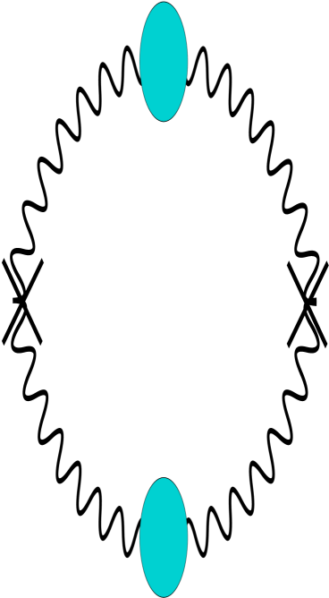
Figure 5: Feynman diagram for the correlator $\langle\Theta_{00}(x)\Theta_{00}(y)\rangle$ in a thermalized, deconfining SU(2) gauge theory including radiative corrections to lowest order. (Blobs signal a resummation of the one-loop polarization for the massless mode.) Crosses denote the insertion of the composite operator $\Theta_{00}$.

3.2 Thermal part of two-point correlation

In analogy to Eq. (2.2) the thermal part $\langle\Theta_{00}(\textbf{x})\Theta_{00}(\textbf{y})\rangle^{\tiny\mbox{th}}$ now calculates as

$$\langle\Theta_{00}({\bf x})\Theta_{00}({\bf y})\rangle^{\tiny\mbox{th}} = \frac{1}{2}\left(\int\!\!\frac{d^{3}p}{(2\pi)^{3}}\sqrt{{\bf p}^{2}+G}\,n_{B}(\beta\sqrt{{\bf p}^{2}+G})\,\mbox{e}^{i{\bf p}({\bf x}-{\bf y})}\right)^{2}$$

$$+\frac{1}{2}\left(\int\!\!\frac{d^{3}p}{(2\pi)^{3}}\frac{{\bf p}^{2}}{\sqrt{{\bf p}^{2}+G}}\,n_{B}(\beta\sqrt{{\bf p}^{2}+G})\,\mbox{e}^{i{\bf p}({\bf x}-{\bf y})}\right)^{2}$$

$$+\frac{1}{2}\int\!\!\frac{d^{3}p}{(2\pi)^{3}}\int\!\!\frac{d^{3}k}{(2\pi)^{3}}\left(\frac{{\bf p}{\bf k}}{|{\bf p}||{\bf k}|}\right)^{2}\sqrt{{\bf p}^{2}+G}\sqrt{{\bf k}^{2}+G}\times$$

$$\ \ \ \ \ \ n_{B}(\beta\sqrt{{\bf p}^{2}+G})n_{B}(\beta\sqrt{{\bf k}^{2}+G})\,\mbox{e}^{i{\bf p}({\bf x}-{\bf y})}\mbox{e}^{i{\bf k}({\bf x}-{\bf y})}$$

$$+\frac{1}{2}\int\!\!\frac{d^{3}p}{(2\pi)^{3}}\int\!\!\frac{d^{3}k}{(2\pi)^{3}}\left(\frac{{\bf p}{\bf k}}{|{\bf p}||{\bf k}|}\right)^{2}\frac{{\bf p}^{2}}{\sqrt{{\bf p}^{2}+G}}\frac{{\bf k}^{2}}{\sqrt{{\bf k}^{2}+G}}\times$$

$$\ \ \ \ \ \ n_{B}(\beta\sqrt{{\bf p}^{2}+G})n_{B}(\beta\sqrt{{\bf k}^{2}+G})\,\mbox{e}^{i{\bf p}({\bf x}-{\bf y})}\mbox{e}^{i{\bf k}({\bf x}-{\bf y})}\,.$$

The integration over the $p_{0}$- and $k_{0}$-coordinates is performed without constraints and just fixes the dispersion law (17). As in the U(1) case we introduce spherical coordinates and evaluate the integrals over the angles analytically. Upon performing the azimuthal integrations for each summand in Eq. (3.2) the respective expression reduces to a square of an integral over the modulus of spatial momentum. This integral is treated in analogy to the derivation of the black-body spectrum in [21]. Employing the modified dispersion law, the integral over momentum-modulus is replaced in favor of an integral over frequency $\omega$. Those values of $\omega$, which yield an imaginary modulus of the spatial momentum due to strong screening, are excluded from the domain of integration. This regime of strong screening is in the range $\omega_{1}<\omega<\omega_{2}$, where $\omega_{1},\omega_{2}$ denote the solutions of the equation

$$\omega^{2}-G(\omega,T,\Lambda)=0\,.$$ (19)

Finally, we introduce a dimensionless frequency $\tilde{\omega}\equiv\beta\omega$ and a dimensionless screening function $\tilde{G}\equiv\beta^{2}G$ and arrive at

$$\langle\Theta_{00}({\bf x})\Theta_{00}({\bf y})\rangle^{\tiny\mbox{th}}=$$

$$\frac{1}{(2\pi)^{6}\beta^{8}}\left(\frac{32\pi^{2}}{3}\left(\int\limits_{0\leq\tilde{\omega}\leq\tilde{\omega}_{1},\atop\tilde{\omega}_{2}\leq\tilde{\omega}\leq\infty}d\tilde{\omega}\left(\tilde{\omega}-\frac{1}{2}\frac{d\tilde{G}}{d\tilde{\omega}}\right)\,\tilde{\omega}\sqrt{\tilde{\omega}^{2}-\tilde{G}}\,\frac{j_{0}(\sqrt{\tilde{\omega}^{2}-\tilde{G}}\,|\tilde{{\bf z}}|)}{e^{\tilde{\omega}}-1}\right)^{2}\right.$$

$$\left.+\,\frac{32\pi^{2}}{3}\left(\int\limits_{0\leq\tilde{\omega}\leq\tilde{\omega}_{1},\atop\tilde{\omega}_{2}\leq\tilde{\omega}\leq\infty}d\tilde{\omega}\left(\tilde{\omega}-\frac{1}{2}\frac{d\tilde{G}}{d\tilde{\omega}}\right)\,\frac{(\sqrt{\tilde{\omega}^{2}-\tilde{G}})^{3}}{\tilde{\omega}}\,\frac{j_{0}(\sqrt{\tilde{\omega}^{2}-\tilde{G}}\,|\tilde{{\bf z}}|)}{e^{\tilde{\omega}}-1}\right)^{2}\right.$$

$$\left.+\,\frac{16\pi^{2}}{3}\left(\int\limits_{0\leq\tilde{\omega}\leq\tilde{\omega}_{1},\atop\tilde{\omega}_{2}\leq\tilde{\omega}\leq\infty}d\tilde{\omega}\left(\tilde{\omega}-\frac{1}{2}\frac{d\tilde{G}}{d\tilde{\omega}}\right)\,\,\tilde{\omega}\sqrt{\tilde{\omega}^{2}-\tilde{G}}\,\frac{j_{2}(\sqrt{\tilde{\omega}^{2}-\tilde{G}}\,|\tilde{{\bf z}}|)}{e^{\tilde{\omega}}-1}\right)^{2}\right.$$

$$\left.+\,\frac{16\pi^{2}}{3}\left(\int\limits_{0\leq\tilde{\omega}\leq\tilde{\omega}_{1},\atop\tilde{\omega}_{2}\leq\tilde{\omega}\leq\infty}d\tilde{\omega}\left(\tilde{\omega}-\frac{1}{2}\frac{d\tilde{G}}{d\tilde{\omega}}\right)\,\frac{(\sqrt{\tilde{\omega}^{2}-\tilde{G}})^{3}}{\tilde{\omega}}\,\frac{j_{2}(\sqrt{\tilde{\omega}^{2}-\tilde{G}}\,|\tilde{{\bf z}}|)}{e^{\tilde{\omega}}-1}\right)^{2}\right)\,.$$

3.3 Estimate for vacuum part of two-point correlation

Here we would like to obtain an order-of-magnitude estimate for the vacuum part of the two-point correlation of $\Theta_{00}$ (massless mode) in deconfining SU(2) Yang-Mills thermodynamics. To do this we ignore the modification of the dispersion law in Eq. (17). Anyways, the function $G$ has so far only been computed for external momentum $p$ with $p^{2}=0$. The difference as compared to the U(1) case is then a restriction of the (euclidean) four-momentum $p$ as $p^{2}\leq|\phi|^{2}$ due to the existence of a scale of maximal resolution $|\phi|$ in the effective theory. Again, we will see that $\langle\Theta_{00}({\bf x})\Theta_{00}({\bf y})\rangle^{\tiny\mbox{vac}}$ is a negligible correction to $\langle\Theta_{00}({\bf x})\Theta_{00}({\bf y})\rangle^{\tiny\mbox{th}}$ for physically interesting distances.

In case of $\langle\Theta_{00}(x)\Theta_{00}(y)\rangle^{\tiny\mbox{vac}}$ we again restrict to $x_{0}=y_{0}$ to be able to compare with $\langle\Theta_{00}(\textbf{x})\Theta_{00}(\textbf{y})\rangle^{\tiny\mbox{th}}$. Introducing the dimensionless version of $\phi$ as $\tilde{\phi}\equiv\beta\phi$, proceeding in a way analogous to the derivation of Eq. (2.3), and performing the $\psi$- and $|\tilde{p}|$-integrations, we arrive at

$$\langle\Theta_{00}({\bf x})\Theta_{00}({\bf y})\rangle^{\tiny\mbox{vac}}\sim$$

$$\frac{1}{(2\pi)^{8}\beta^{8}}\Bigg{(}96\pi^{2}\cdot\frac{\pi^{2}}{|{\bf\tilde{z}}|^{8}}\left(2J_{0}(|{\bf\tilde{z}}||\tilde{\phi}|)+|{\bf\tilde{z}}||\tilde{\phi}|J_{1}(|{\bf\tilde{z}}||\tilde{\phi}|)-2\right)^{2}$$

$$+ \left.48\pi^{2}\cdot\frac{\pi^{2}}{4|{\bf\tilde{z}}|^{8}}\left(2(8J_{0}(|{\bf\tilde{z}}||\tilde{\phi}|)+|{\bf\tilde{z}}||\tilde{\phi}|J_{1}(|{\bf\tilde{z}}||\tilde{\phi}|)-8)+3|{\bf\tilde{z}}|^{2}|\tilde{\phi}|^{2}\,\,_{1}F_{2}\left(\frac{1}{2};\frac{3}{2},2;-\frac{|{\bf\tilde{z}}|^{2}|\tilde{\phi}|^{2}}{4}\right)\right)^{2}\right.$$

$$+ \left.\frac{32\pi^{2}}{3}\cdot\frac{\pi^{2}}{|{\bf\tilde{z}}|^{8}}\left((|{\bf\tilde{z}}|^{2}|\tilde{\phi}|^{2}-2)J_{0}(|{\bf\tilde{z}}||\tilde{\phi}|)-3|{\bf\tilde{z}}||\tilde{\phi}|J_{1}(|{\bf\tilde{z}}||\tilde{\phi}|)+2\right)^{2}\right.$$

$$+ \left.\frac{16\pi^{2}}{3}\cdot\frac{\pi^{2}}{|{\bf\tilde{z}}|^{8}}\left((|{\bf\tilde{z}}|^{2}|\tilde{\phi}|^{2}-8)J_{0}(|{\bf\tilde{z}}||\tilde{\phi}|)-6|{\bf\tilde{z}}||\tilde{\phi}|J_{1}(|{\bf\tilde{z}}||\tilde{\phi}|)+8\right)^{2}\right.$$

$$+ \left.32\pi^{2}\cdot\frac{\pi^{2}|\tilde{\phi}|^{8}}{64}\left(\,\,{}_{1}F_{2}\left(\frac{1}{2};\frac{3}{2},3;-\frac{|{\bf\tilde{z}}|^{2}|\tilde{\phi}|^{2}}{4}\right)\right)^{2}\right.$$

$$+ \left.24\pi^{2}\cdot\frac{\pi^{2}|\tilde{\phi}|^{4}}{|{\bf\tilde{z}}|^{4}}\left(J_{2}(|{\bf\tilde{z}}||\tilde{\phi}|)\right)^{2}\right.$$

$$+ 48\pi^{2}\cdot\frac{\pi^{2}|\tilde{\phi}|^{2}}{4|{\bf\tilde{z}}|^{6}}\left(6J_{1}(|{\bf\tilde{z}}||\tilde{\phi}|)+2|{\bf\tilde{z}}||\tilde{\phi}|J_{2}(|{\bf\tilde{z}}||\tilde{\phi}|)-3|{\bf\tilde{z}}||\tilde{\phi}|\,\,_{1}F_{2}\left(\frac{1}{2};\frac{3}{2},2;-\frac{|{\bf\tilde{z}}|^{2}|\tilde{\phi}|^{2}}{4}\right)\right)^{2}\Bigg{)}\,,$$

where $\,{}_{1}F_{2}$ is a hypergeometric function and $J_{0},J_{1},J_{2}$ are Bessel functions of the first kind (conventions as in [40]).

3.4 Numerical results

The integral in Eqs. (3.2) is evaluated numerically. Let us first compare the estimate for the vacuum contribution in Eq. (3.3) with the thermal part of the correlator $\langle\Theta_{00}({\bf x})\Theta_{00}({\bf y})\rangle$. To make contact with SU(2)${}_{\tiny\mbox{CMB}}$, whose Yang-Mills scale is $\Lambda=1.065\times 10^{-4}$ eV [16, 21], we relate at a given temperature the dimensionless distance $|\tilde{{\bf z}}|$ to the physical distance in centimeters. We define

$$R_{\tiny\mbox{th}-\tiny\mbox{vac};\tiny\mbox{SU(2)}}(|{\bf z}|)\equiv\frac{\langle\Theta_{00}({\bf x})\Theta_{00}({\bf y})\rangle^{\tiny\mbox{th}}}{\left|\langle\Theta_{00}({\bf x})\Theta_{00}({\bf y})\rangle^{\tiny\mbox{vac}}\right|}\,,$$ (22)

where we use the estimate in Eq. (3.3) for $\left|\langle\Theta_{00}({\bf x})\Theta_{00}({\bf y})\rangle^{\tiny\mbox{vac}}\right|$. In Fig. 6 the quantity $R_{\tiny\mbox{th}-\tiny\mbox{vac};\tiny\mbox{SU(2)}}(|{\bf z}|)$ is depicted for various temperatures specializing to the case of SU(2)${}_{\tiny\mbox{CMB}}$. Here we have used the one-loop selfconsistent determination of the function $G$ such that $G=p^{2}$, see [41]. The thus obtained improvement of $G$ shows that $\tilde{\omega}_{1}\equiv 0$ in Eq. (3.2).

Notice the strong dominance of the thermal part. Notice also that although this result resembles qualitatively the result of Fig. 2 for fixed distance and varying temperature this is not true for fixed temperature and varying distance. Namely, the existence of a nontrivial thermal ground state in deconfining SU(2) Yang-Mills thermodynamics constrains quantum fluctuations of the massless mode to be softer than the scale $|\phi|$. Owing to its trivial ground state, no such constraint exists in a thermalized U(1) gauge theory. As a consequence and in accord with Fig. 2, quantum fluctuations dominate thermal fluctuations at small distances in such a theory.

By virtue of the results shown in Fig. 2 and Fig. 6 we neglect the vacuum contribution to $\langle\Theta_{00}({\bf x})\Theta_{00}({\bf y})\rangle$ in the following.

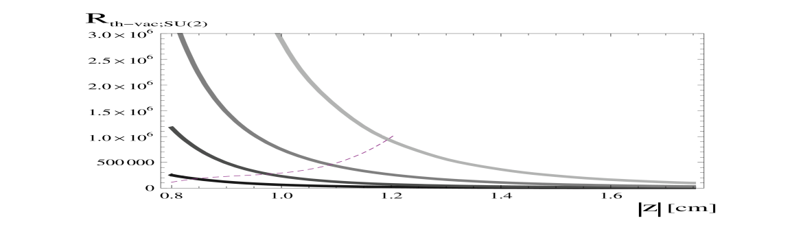
Figure 6: The function $R_{\tiny\mbox{th}-\tiny\mbox{vac};\tiny\mbox{SU(2)}}(|{\bf z}|)$, defined as in Eq. (22), when specializing to the case of SU(2)${}_{\tiny\mbox{CMB}}$ ($T_{c}=2.73\,$K), for various temperatures: black curve ($T=1.5\,T_{c}$), dark grey curve ($T=2.0\,T_{c}$), grey curve ($T=2.5\,T_{c}$), light grey curve ($T=3.0\,T_{c}$). The dashed line separates distances smaller than $|\phi|^{-1}$ from those that are larger than $|\phi|^{-1}$.

Let us now turn to the interesting question of how much suppression there is in the correlation of the photon energy density in the case of SU(2)${}_{\tiny\mbox{CMB}}$ as compared to the conventional U(1) case. In Fig. 7 the ratio $R_{\tiny\mbox{th,SU(2)}-\tiny\mbox{th,U(1)}}(|{\bf z}|)$, defined as

$$R_{\tiny\mbox{th,SU(2)}-\tiny\mbox{th,U(1)}}(|{\bf z}|)\equiv\frac{\langle\Theta_{00}({\bf x})\Theta_{00}({\bf y})\rangle^{\tiny\mbox{th,SU(2)}}}{\langle\Theta_{00}({\bf x})\Theta_{00}({\bf y})\rangle^{\tiny\mbox{th,U(1)}}}\,,$$ (23)

is depicted for various temperatures as a function of distance in centimeters. Again we have used the one-loop selfconsistent determination of the function $G$ such that $G=p^{2}$, see [41].

Figure 7: The function $R_{\tiny\mbox{th,SU(2)}-\tiny\mbox{th,U(1)}}(|{\bf z}|)$, as defined in Eq. (23), when specializing to the case of SU(2)${}_{\tiny\mbox{CMB}}$ ($T_{c}=2.73\,$K), for various temperatures: black curve ($T=1.5\,T_{c}$), dark grey ($T=2.0\,T_{c}$), grey ($T=2.5\,T_{c}$), light grey ($T=3.0\,T_{c}$). Notice the regime of antiscreening for small $|z|$. For $T=3.0\,T_{c}$, where the approximation $p^{2}=0$ deviates sizably from the full result for the screening function $G$, we have used $G$ as obtained 1-loop selfconsistently [41].

Notice the suppression of the correlation between photon energy densities in the case of an underlying SU(2) gauge symmetry as compared to the case of the conventional U(1). Since the correlator $\langle\Theta_{00}({\bf x})\Theta_{00}({\bf y})\rangle$ is a measure for the energy transfer between the spatial points ${\bf x}$ and ${\bf y}$ in thermal equilibrium and hence a measure for the interaction of microscopic objects emitting and absorbing radiation, we conclude that this interaction is, as compared to the conventional theory, suppressed on distances $\sim 1\,$cm if photon propagation is subject to an SU(2) gauge principle.

4 Stability of clouds of atomic hydrogen in the Milky Way

The results of Sec. 3 have immediate implications for the gradual metamorphosis of cold ($T=5\dots 10\,$K) astrophysical objects such as the hydrogen cloud GSH139-03-69 observed in between spiral arms of the outer Milky Way [28]. This object possesses an estimated age of about 50 million years, exhibits a brightness temperature $T_{B}$ of $T_{B}\sim 20\,$K with cold regions of $T_{B}\sim 5\cdots 10\,$K and an atomic number density of $\sim 1.5\,$cm^-3. The puzzle about this and similar structures seems to be its high content of atomic hydrogen in view of its unexpectedly large age. Namely, numerical simulations of the cloud evolution subject to standard interatomic forces suggest a much lower time scale of less than 10 million years, see [42, 43, 44] and references therein, for the generation of a substantial fraction of H₂ molecules.

Although a quantitative estimate of the increased stability of atomic hydrogen clouds due to the SU(2) effects in thermalized photon propagation is beyond the scope of the present work, Fig. 7 clearly expresses that the mean energy transfer in the photon gas of $T=5\cdots 10\,$K is suppressed by up to a factor of two at the interatomic distances in the hydrogen cloud GSH139-03-69. This, however, implies that atomic interactions, leading to the formation of molecules, are strongly suppressed. It would be interesting to see how the simulation of the cloud evolution, taking into account the effects as expressed in Fig. 7, would increase the estimate for its age as compared to the standard picture.

As already pointed out in [21], the propagation of the 21-cm line is unscreened even when subjecting photons to SU(2)${}_{\tiny\mbox{CMB}}$. However, a recent full calculation of $G$ shows that this result is an artefact of the approximation $p^{2}=0$ [41]: Thermalization of the hydrogen cloud thus takes place solely via the coupling of the photon to the nontrivial thermal ground state [45].

5 Summary and Conclusions

In this work we have computed the two-point correlation of the canonical energy density of photons both in the conventional and postulated case of a U(1) and SU(2) gauge group, respectively. In the real-time formalism of finite-temperature field theory and resumming the polarization tensor for the massless mode (photon) [16] in the SU(2) case, this correlation splits into a thermal and a vacuum part. We have observed that for the case of SU(2)${}_{\tiny\mbox{CMB}}$, which is postulated to be the nonabelian gauge theory underlying photon propagation [20, 21, 24], the vacuum part is strongly suppressed as compared to the thermal part for distances $\sim 1$ cm. Furthermore, there is strong suppression of the SU(2)${}_{\tiny\mbox{CMB}}$-correlator as compared to the U(1)-correlator at the interatomic distances of hydrogen atoms within unexpectedly stable and cold ($T\sim 5\cdots 10\,$K) cloud structures in between spiral arms of the Milky Way. Thus the mean energy transport and hence the atomic interactions are hamstrung in such structures possibly explaining their unsuspectedly large age.

To make the situation even more explicit we have computed the Coulomb potential $V(r)$ ($r\equiv|{\bf x}|$) of a heavy point charge in case of photons being described by a U(1) and an SU(2) gauge theory. This potential is given in a U(1) theory as

$$V_{\tiny\mbox{U(1)}}(r) = \frac{1}{(2\pi)^{3}}\int d^{3}p\,\frac{\mbox{e}^{-i{\bf p}\cdot{\bf x}}}{{\bf p}^{2}}=\frac{1}{2\pi^{2}}\int_{0}^{\infty}dp\,\frac{\sin pr}{pr}=\frac{1}{2\pi^{2}r}\int_{0}^{\infty}d\xi\,\frac{\sin\xi}{\xi}$$ (24)

$$= \frac{1}{4\pi r}\,.$$

Going from U(1) to SU(2), we take into account the resummed one-loop polarization [16] by letting ${\bf p}^{2}\to{\bf p}^{2}+G$ in the denominator of the integrand in Eq. (24). Here $G$ is the same function as discussed in Sec. 3.1. The physical situation is a heavy point charge immersed into the SU(2) plasma with the photons associated with it being (anti)screened by nonabelian, thermal fluctuations. Although the function $G$ is known for on-shell photons $\omega^{2}={\bf p}^{2}$ only this recipe should work well for sufficiently large distances since the off-shellness of the photon, which does not mediate any energy transfer from the source, then is sufficiently small. Thus for SU(2) we approximately have

$$V_{\tiny\mbox{SU(2)}}(r) = \frac{1}{(2\pi^{3})}\int d^{3}p\,\frac{\mbox{e}^{-i{\bf p}\cdot{\bf x}}}{{\bf p}^{2}+G(T,|{\bf p}|,\Lambda)}$$ (25)

$$= \frac{1}{2\pi^{2}r}\int_{0}^{\infty}dp\,\frac{p}{p^{2}+G(T,p,\Lambda)}\sin pr\,,$$

where the last integral is performed numerically. In Fig. 8 both potentials, $V_{\tiny\mbox{U(1)}}(r)$ and $V_{\tiny\mbox{SU(2)}_{\tiny\mbox{CMB}}}(r)$, as well as their ratio are plotted as functions of $r$.

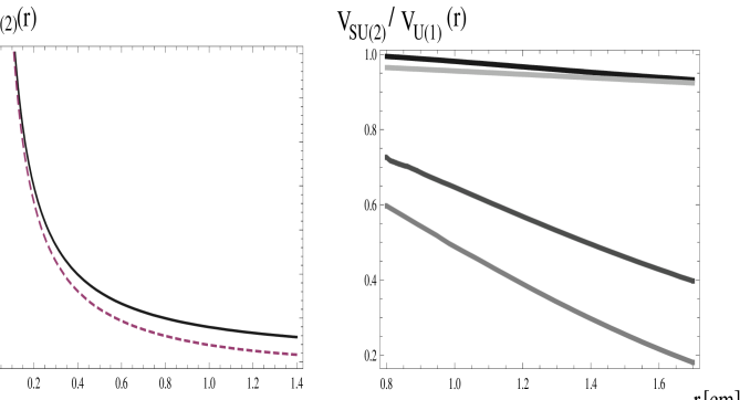
Figure 8: Left panel: Plot of the potentials $V_{\tiny\mbox{U(1)}}(r)$ (dashed line) and $V_{\tiny\mbox{SU(2)}_{\tiny\mbox{CMB}}}(r)$ (solid line) as a function of $r$ at $T=2.5\,T_{\tiny\mbox{CMB}}\sim 6.8$ K. Right panel: Plot of the ratio $V_{\tiny\mbox{SU(2)}_{\tiny\mbox{CMB}}}(r)/V_{\tiny\mbox{U(1)}}(r)$ as a function of $r$. The temperature is set to $T=1.5\,T_{c}$ (black), $T=2.0\,T_{c}$ (dark grey), $T=2.5\,T_{c}$ (grey), and $T=3.0\,T_{c}$ (light grey). For $T=3.0\,T_{c}$, where the approximation $p^{2}=0$ deviates sizably from the full result for the screening function $G$, we have used $G$ as obtained 1-loop selfconsistently [41]. Notice how close to unity the curve at $T=3.0\,T_{c}$ is as compared to the curve at $T=2.5\,T_{c}$ for the right-hand side panel.

Notice that the dimensionless quantity $V_{\tiny\mbox{SU(2)}_{\tiny\mbox{CMB}}}(r)/V_{\tiny\mbox{U(1)}}(r)$ shows similar suppression as the dimensionless quantity $R_{\tiny\mbox{th,SU(2)}-\tiny\mbox{th,U(1)}}(|{\bf z}|)$ depicted in Fig. 7. This seems to confirm the validity of our above approximation. However, we wish to stress that such a simple approximation cannot be used in a general framework: Apart from the partial knowledge of the function $G$ (known on-shell only) our thermodynamical approach to SU(2)${}_{\tiny\mbox{CMB}}$ and its application to the screening of Coulomb potnetials breaks down when macroscopic sources with large multiples of the elementary electric charge are considered. In fact, in this case large energy densities ($\rho\gg T^{4}$) are locally present which destroy the applicability of a thermalized theory. But the effective, Debye massive nature of the photon can only be detected in weakly adulterated thermal systems (black body) [21] and is relevant in the cold atomic hydrogen clouds as discussed in this work.

References

- [1] A. D. Linde, Phys. Lett. B 108, 389 (1982).
- [2] A. M. Polyakov, Phys. Lett. B 59, 82 (1975).
- [3] D. J. Gross, R. D. Pisarski, and L. G. Yaffe, Rev. Mod. Phys. 53, 43 (1981).
- [4] K. Kajantie, M. Laine, K. Rummukainen, and Y. Schroder, Phys. Rev. D 67, 105008 (2003) [hep-ph/0211321].
- [5] C. Zhai and B. Kastening, Phys. Rev. D 52, 7232 (1995) [hep-ph/9507380].
- [6] P. Arnold and C. Zhai, Phys. Rev. D 50, 7603 (1994) [hep-ph/9408276], ibid. D 51, 1906 (1995) [hep-ph/9410360].
- [7] T. Toimela, Phys. Lett. B 124, 461 (1983).
- [8] J. I. Kapusta, Nucl. Phys. B 148, 461 (1979).
- [9] E. V. Shuryak, Sov. Phys. JETP 47, 212 (1978).
- [10] S. A. Chin, Phys. Lett. B 78, 552 (1978).
- [11] R. Hofmann, Int. J. Mod. Phys. A20 (2005) 4123; Erratum-ibid. A21 (2006) 6515.
- [12] U. Herbst and R. Hofmann, hep-th/0411214.
- [13] C. P. Korthals Altes (Marseille, CPT), in *Minneapolis 2006, Continuous advances in QCD* 266-272 [hep-ph/0607154].
- [14] C. Korthals-Altes and A. Kovner, Phys. Rev. D 62, 096008 (2000) [hep-ph/0004052].
- [15] C. Korthals-Altes, hep-ph/0406138.
- [16] M. Schwarz, R. Hofmann, and F. Giacosa, Int. J. Mod. Phys. A 22, 1213 (2007) [hep-th/0603078].
- [17] R. Hofmann, arXiv:0710.0962v2 [hep-th].
- [18] D. Kaviani and R. Hofmann, Mod. Phys. Lett. A22, (2007) 2343.
- [19] R. Hofmann, hep-th/0609033.
- [20] R. Hofmann, PoS JHW2005, 021 (2006) [hep-ph/0508176].
- [21] M. Schwarz, R. Hofmann, and F. Giacosa, JHEP 0702, 091 (2007) [hep-ph/0603174].
- [22] M. Szopa and R. Hofmann, JCAP 0803, 001 (2008).
- [23] M. Szopa, R. Hofmann, F. Giacosa, and M. Schwarz, Eur. Phys. J. C 54, 655 (2008).
- [24] F. Giacosa and R. Hofmann, Eur. Phys. J. C50, 635 (2007) [hep-th/0512184].
- [25] S. L. Adler, Phys. Rev. 177, 2426 (1969).
- [26] S. L. Adler and W. A. Bardeen, Phys. Rev. 182, 1517 (1969).
- [27] J. S. Bell and R. Jackiw, Nuovo Cim. A60, 47 (1969).
- [28] L. B. G. Knee and C. M. Brunt, Nature 412, 308 (2001).
- [29] U. Herbst, R. Hofmann, J. Rohrer, Acta Phys. Polon. B36, 881 (2005) [hep-th/0410187].
- [30] G. ’t Hooft, Nucl. Phys. B79, 276 (1974).
- [31] J. Keller, Diploma thesis Universität Heidelberg, arXiv:0801.3961 [hep-th].
- [32] B. J. Harrington and H. K. Shepard, Phys. Rev. D 17, 2122 (1978).
- [33] W. Nahm, Phys. Lett. B90 413 (1980).
- [34] W. Nahm, Lect. Notes in Physics 201 189 (1984), eds. G. Denaro.
- [35] K.-M. Lee, C.-H. Lu, Phys. Rev. D 58 025011 (1998).
- [36] T. C. Kraan and P. van Baal, Nucl. Phys. B 533 627 (1998).
- [37] T. C. Kraan and P. van Baal, Phys. Lett. B 428 268 (1998).
- [38] T. C. Kraan and P. van Baal, Phys. Lett. B 435 389 (1998).
- [39] R. C. Brower , D. Chen, J. Negele, K. Orginos, C.-I. Tan, Nucl. Phys. Proc. Suppl. 73 557 (1999).
- [40] I. S. Gradshteyn and I. M. Ryzhik, Table of Integrals, Series, and Products, Academic Press, New York and London (1965).
- [41] J. Ludescher and R. Hofmann, arXiv:0806.0972 [hep-th].
- [42] P. Goldsmith, D. Li, and M. Kro, Astrophys. J. 654, 273 (2007).
- [43] D. M. Meyer and J. T. Lauroesch, Astrophys. J. 650 (2006) L67 [arXiv:astro-ph/0609611].
- [44] S. Redfield and J. L. Linsky, arXiv:0709.4480 [astro-ph].
- [45] J. Ludescher, J. Keller, F. Giacosa, and R. Hofmann, work in progress.