Iterative Filtering
for a Dynamical Reputation System

Abstract.

The paper introduces a novel iterative method that assigns a reputation to $n+m$ items: $n$ raters and $m$ objects. Each rater evaluates a subset of objects leading to a $n\times m$ rating matrix with a certain sparsity pattern. From this rating matrix we give a nonlinear formula to define the reputation of raters and objects. We also provide an iterative algorithm that superlinearly converges to the unique vector of reputations and this for any rating matrix. In contrast to classical outliers detection, no evaluation is discarded in this method but each one is taken into account with different weights for the reputation of the objects. The complexity of one iteration step is linear in the number of evaluations, making our algorithm efficient for large data set. Experiments show good robustness of the reputation of the objects against cheaters and spammers and good detection properties of cheaters and spammers.

1. Introduction

There is an important growth of sites on the World Wide Web where users play a crucial role: they provide trust ratings to objects or even to other raters. Such sites may be commercial, where buyers evaluate sellers or articles (Ebay, Amazone, etc.), or they may be opinion sites, where users evaluate objects (Epinions, Tailrank, MovieLens, etc.). But websites are not the only place where we can find ratings between users and items: the simple fact to link to another webpage is considered by search engines as a positive evaluation (Google, Yahoo, etc.). Therefore the good working of auction systems, opinion websites, search engines, etc. depends directly on the reliability of their raters and on the treatment of all the data. Trust and reputation in the electronic market gives a necessary transparency to their users. For example, in 1970, Akerloff [7] pointed out the information asymmetry between the buyers and the sellers in the market for lemons. The former had more information than the latter, making hard trusting trading relationships. From what precedes, two questions naturally arises:

- What should be the reputation of the evaluated items?
- How can we measure the reliability of the raters?

We will distinguish the reputation, that is what is generally said or believed about a person’s or thing’s character or standing, and the reliability, that is the subjective probability by which one expects that a rater gives an evaluation on which its welfare depends. Let us remark that many technics only calculate the reputations of items. Sometimes reputation and reliability have the same value as it is the case in eigenvector based technic where the reputation of any individual depends on the reputations of his raters [5, 8]. In these methods, they construct a stochastic matrix from the network and the ratings, then the eigenvector of that matrix gives the reputations. Another part of the literature concerns the propagation of trust (and distrust) [6, 10, 9, 11] where they define trust metrics between pairs of individuals $(A,B)$ looking at the possible paths linking $A$ with $B$. So reputations depend on the point of view of the user and these methods differ from ours that assigns one global reputation for each item.

Our method weights the evaluations of the raters. A small weight is a natural way to tackle the problem of attackers in reputation systems. Therefore, the method gives two values for a user: his reputation depending on his received evaluations and his weight that influence the impact of his given evaluations. The algorithm is based on an iterative refinement that is guarantied to converge to a reputation score and a reliability score for each item: at each step the reliability of a rater is calculated according to some distance between his given evaluations and the reputations of the items he evaluates. This distance is interpreted as the belief divergence. Typically, a rater diverging to much from the group will be distrusted after convergence. The same definition of distance appears in [1, 2, 3] and is used for the same issue. In [1], the function that determines the weights is different. This difference makes their algorithm sensitive to initial conditions without any guaranty of convergence. Moreover, they are in the less general case where it is supposed that every rater evaluates all items. In [2], they want to tackle the problem of spammers in collaborative filtering where previous evaluations are used to predict future evaluations. Again the same definition of distance allows to penalize the divergent raters. Even though the function that assigns the weights for the evaluations is the same, there is no iterative procedure but only a simple step is applied. In [3], they use another function to determine the weights: the log-likelihoods, but again only a simple step is applied. We show in section 3 the advantage to apply more than one step in the iterative filtering. Indeed, each step separates a little more the outliers.

Let us remark that beside the refinement process of the reputations and the outlier detection given by our procedure, other applications can take advantage of these data. For example, [2] want to remove spammers to improve collaborative filtering. Similarly in [4], they propose a framework to take into account the different qualities of ratings for collaborative filtering. Hence they weight each rating according to its reliability, these weights can be those obtained by the iterative filtering we described.

In the sequel, we first explain in section 2 how the reputation vector for the objects and the weights for the evaluation are built. Moreover, we develop the algorithm Reputation that calculates these values, and we explain its interpretation and its properties of convergence. Then in section 3, our experiments test the robustness of our method against attackers and show several iterations on graphics. Finally in section 4, we point out possible extensions and experiments for our method.

2. The iterative method

Before to develop the model and the algorithm, we introduce the main notations in the following tabular.

  Notations    Definitions $n$, $m$, $m_{i}$ # of raters,# of items, # of items evaluated by $i$. $E$ The $n\times m$ rating matrix: $E_{ij}$ is the evaluation given by rater $i$ to item $j$ $A$ The $n\times m$ adjacency matrix: $A_{ij}=1$ if rater $i$ evaluates $j$, otherwise $A_{ij}=0$ (and $E_{ij}=0$) $T$ The $n\times m$ trust matrix of evaluations $t$ The $n\times 1$ trust vector of raters $r$ The $m\times 1$ reputation vector of items 1 The $n\times 1$ or $m\times 1$ vector of ones $\sum_{i,\>i\rightarrow j}$ Sum over the set $\{i|A_{ij}=1\}$ $\sum_{j,\>i\rightarrow j}$ Sum over the set $\{j|A_{ij}=1\}$

Without loss of generality, we will consider ratings in the interval $[0,1]$, i.e. $E\in[0,1]^{n\times m}$ and therefore the reputation vector $r$ will belong to $[0,1]^{m}$. Moreover, the trust matrix $T$ and the trust vector $t$ are nonnegative, i.e. the entries of $T$ and $t$ are nonnegative.

2.1. The model

As already said in the introduction, the reputations of the items essentially depend on the evaluations they receive. These latter are weighted according to their reliability. In that way, the reputation of item $j\in\{1,\dots,m\}$ is obtained by taking the weighted sum of its evaluations, i.e.

(1) $$r_{j}=\sum_{i,\>i\rightarrow j}W_{ij}E_{ij},\quad\sum_{i,\>i\rightarrow j}W_{ij}=1$$

And we define the matrix $W$ from the trust matrix $T$ in the following way:

(2) $$W_{ij}=\frac{T_{ij}}{\sum_{k,\>k\rightarrow j}T_{kj}},\quad i=1,\dots,n,\quad j=1\dots,m.$$

In that manner, evaluations with a higher trust value are taken into account more for the reputation vector. Now the important role is played by the trust matrix $T$, its definition is given in the next section.

2.2. The trust matrix

Let us describe the trust matrix that assigns a measure of confidence to each rating. The inputs of the trust matrix are the rating matrix $E$ and the reputation vector $r$. Formally, we define the belief divergence of rater $i\in\{1,\dots,n\}$ as the estimated variance of the $i^{th}$ row of $E$:

(3) $$d_{i}=\frac{1}{m_{i}}\sum_{j,\>i\rightarrow j}(E_{ij}-r_{j})^{2},$$

where $m_{i}$ is the number of items evaluated by $i$. That definition is somewhat similar to the one proposed in [2] where $d$ is used to penalize those raters that have an high belief divergence. The resulting trust matrix is

(4) $$T_{ij}=c_{j}-d_{i},$$

for any evaluation from $i$ to $j$. The parameters $c_{j}$ are chosen such that the entries of $T$ are nonnegative. Moreover $c_{j}$ are discriminating in the sense that they influence the ratios $T_{ij}/T_{kj}$ for $i,k\in\{1,\dots,n\}$ and $j\in\{1,\dots,m\}$. Typically, the smaller $c_{j}$, the more spammers evaluating object $j$ are penalized. In order to have a trust value for each raters, we also define the trust vector $t$:

(5) $$t_{i}=d_{max}-d_{i},$$

where $d_{max}$ is the maximum of the elements of the vector $d$.

2.3. The algorithm

From equations (1-5), we can derive the algorithm [r t] = Reputation(E,A,c) that takes as inputs a rating matrix $E$, an adjacency matrix $A$ and a $m\times 1$ vector $c$ of parameters. Then it iteratively calculates the reputation vectors $r$ and the trust matrix $T$. Eventually, the algorithm gives the reputation and the trust vector. The description is given in four steps corresponding to the initialization, two updates for $r$ and $T$ and the calculation of the trust vector $t$.

• Initialization of matrix $T$: every rater is evenly trusted, i.e. $T_{ij}=1$ for $i=1,\dots,n$ and $j=1,\dots,m$.
  

• The matrix of weights and the reputation vector are calculated from $T$. For $i=1,\dots,n$ and $j=1,\dots,m$:

  $$W_{ij}=\frac{T_{ij}}{\sum_{k,\>k\rightarrow j}T_{kj}},\quad\quad r_{j}=\sum_{i,\>i\rightarrow j}W_{ij}E_{ij}.$$

• The belief divergence and the new trust matrix are calculated from $r$. For $i=1,\dots,n$ and $j=1,\dots,m$:

  $$d_{i}=\frac{1}{m_{i}}\sum_{j,\>i\rightarrow j}(E_{ij}-r_{j})^{2},\quad\quad T_{ij}=c_{j}-d_{i}.$$

  If the $i^{th}$ row of $T$ is zero, then replace it by a row of ones.
  Repeat steps (ii) and (iii) until convergence.
  

• The trust vector $t$ is given by $\max_{k}d_{k}-d_{i}$.

Let us remind that the input parameters $c$ used in step (iii) are chosen sufficiently large such that the entries of $T$ are nonnegative at each iteration.

$$\begin{array}[]{ccccc}\small\textit{Trust}&&&&\small\textit{Weight}\\ \small\textit{for each rating}&\bf{T}&\rightarrow&\bf{W}&\small\textit{for each rating}\\ &\uparrow&&\downarrow&\\ \small\textit{Belief divergence}&\bf{d}&\leftarrow&\bf{r}&\small\textit{Reputation}\\ \small\textit{for each rater}&&&&\small\textit{for each item}\end{array}$$

Figure 1. Cycle of one iteration of the algorithm.

One iteration of the algorithm Reputation is schematized in figure 1. A slight modification allows dynamical evaluations. In that case, the rating matrix $E$ changes at each iteration, i.e. $E[k]$ with $k=1,2,\cdots$. A direct way to update $r$, $T$ and $t$, is given when the first step takes as initial vector the previous trust matrix, and steps (ii) and (iii) are not repeat until convergence, but a certain number of times.

2.4. Interpretation of the solution

The algorithm in section 2.3 converges to the unique solution of equations (1-4), see next section. Let $r^{*}$ represents that solution and for the sake of simplicity, let parameters $c_{j}$ be equals to a same constant $c_{0}$. Then $r^{*}$ is the maximizer of the following scalar function: $\psi:[0,1]^{m}\rightarrow\mathbb{R}$ with

(6) $$\psi(r) = \sum_{i=1}^{n}\sum_{j,\>i\rightarrow j}T_{ij}^{2}$$

(7) $$= \sum_{i=1}^{n}m_{i}\left(c_{0}-\frac{1}{m_{i}}\sum_{j,\>i\rightarrow j}(E_{ij}-r_{j})^{2}\right)^{2}.$$

It is indeed enough to observe that $\text{grad }\psi(r^{*})=0$. In other words, $r^{*}$ maximizes the Frobenius norm of the sparse trust matrix $T$. Maximizing such a norm roughly means that some total degree of confidence over the raters is maximized. More formally, let assume that the entries $E_{ij}$ are i.i.d.$\sim N(r_{j},\sigma^{2})$. In that case, the degree of confidence we can have in evaluation $E_{ij}$ is given by

$$\log Pr(E_{ij}|r_{j})=\textnormal{cst}-\frac{1}{2\sigma^{2}}(E_{ij}-r_{j})^{2},$$

and by summing the evaluations of $i$ and choosing the appropriate constant, we obtain the relation

$$T_{ij}=\frac{2\sigma^{2}}{m_{i}}\sum_{k,\>k\rightarrow j}\log Pr(E_{ij}|r_{j}).$$

In other words, the trust matrix is the normalized sum of the degrees of confidence we have in the evaluations of the raters. Then the maximizer of the Frobenius norm of $T$ is

$$r^{*}=\arg\max_{r\in[0,1]^{m}}\sum_{i=1}^{n}\frac{1}{m_{i}}\left(\sum_{j,\>i\rightarrow j}\log Pr(E_{ij}|r_{j})\right)^{2}.$$

Another writing of the function $\psi$ leads to

$$\psi(r)=-2c_{0}\sum_{i=1}^{n}\sum_{j,\>i\rightarrow j}(E_{ij}-r_{j})^{2}+\sum_{i=1}^{n}\frac{1}{m_{i}}\left(\sum_{j,\>i\rightarrow j}(E_{ij}-r_{j})^{2}\right)^{2},$$

and the maximizer of the first expression is simply the average of the evaluations for each item $j$, i.e. $\sum_{i,\>i\rightarrow j}E_{ij}/|i,\>i\rightarrow~{}j|$, and the maximizer of the second expression necessarily belongs to the border of the hyper cube, i.e. $\{0,1\}^{m}$. The solution $r^{*}$ is then a compromise between both terms in which the parameters $c_{0}$ plays the role of a weighting factor. For large $c$, the algorithm will give the average of the evaluations for each item.

2.5. Properties of convergence

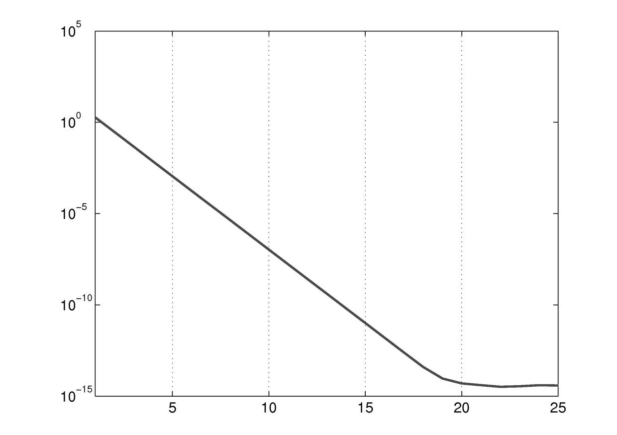
Figure 2. X-Axis: # of iterations. Y-Axis: the euclidian norm of the error, i.e. $\|r[k]-r^{*}\|_{2}$. The graphic was obtained from a $943\times 1682$ sparse rating matrix representing $10^{5}$ evaluations.

In this section we analyze the convergence of Reputation given in section 2.3 and its rate of convergence. For the sake of clearness, we restrict ourselves to the main and important steps in the proof avoiding the technical points.

Theorem 1.

For $c_{j}$ chosen such that the matrix $T$ is nonnegative at each step, the iteration in the algorithm Reputation(E,A,c) converges to the unique vector $r^{*}$.

Proof.

(Only a sketch). For the sake of simplicity, we let parameters $c_{j}$ be equals to a same constant $c_{0}$. We first prove the unicity of $r^{*}$ and then we prove the convergence result.

It can be shown that the scalar function $\psi:[0,1]^{m}\rightarrow\mathbb{R}:r\mapsto\psi(r)$ defined in (7) is continuous and quasiconcave. It has therefore a unique maximizer on $[0,1]^{m}$ that corresponds to the vector $r^{*}$.

Let $r_{k}$ and $r_{k+1}$ be two successive iterations of $r$. It can be shown by simple developments that these two vectors are linked by the following expression:

(8) $$r_{k+1}=r_{k}+\alpha(r_{k})\cdot\textnormal{grad }\psi(r_{k}),$$

where $\alpha(r_{k})\geq(4c_{0})^{-1}>0$ and $\textnormal{grad }\psi(r_{k})$ is the gradient of $\psi$ in $r_{k}$ pointing to the direction of greatest ascent. Therefore one iteration corresponds to take the direction of greatest ascent and make a step of length $\ell_{k}=\alpha(r_{k})\cdot\|\textnormal{grad }\psi(r_{k})\|_{2}$. Moreover, it can be shown that $\ell_{k}$ is such that we have strict ascent:

$$\psi(r[k])<\psi(r[k+1]).$$

Finally, $\ell_{k}$ is also lower bounded by $(4c_{0})^{-1}\|\textnormal{grad }\psi(r[k])\|_{2}$ and therefore the iteration on $r$ monotonically converges to the maximizer of $\psi$ on $[0,1]^{m}$. ∎

Numerical experiments show a linear rate of convergence for the vector $r$. As shown in Figure 2, the logarithm of the error decreases linearly and stabilizes after $20$ steps. It is possible to speed up the rate of convergence by using a Newton method provided that we are close enough to $r^{*}$. Then the rate of convergence becomes quadratic making our algorithm efficient for large data set.

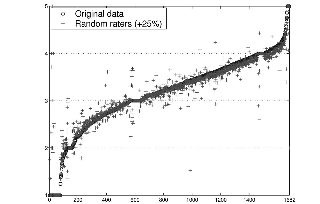
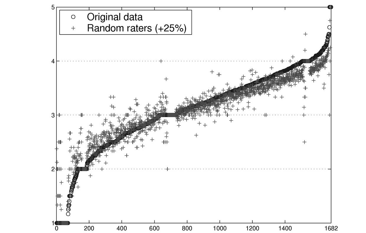
Figure 3. X-Axis: the sorted movies according to their reputations before the addition of random raters. Y-Axis: their reputations according to our algorithm (Top) and to the average (Bottom).

3. Experiments

Our experiment concerns a data set of 100,000 evaluations given by 943 users on 1682 movies and raging from $1$ to $5$. Each user has rated at least 20 movies.

In order to simulate the robustness of the algorithm Reputation, two types of behavior are analyzed in the sequel: first, raters that give random evaluations, and second, spammers that try to improve the reputation of their preferred item.

3.1. Robustness against random raters

We added to the original data set $237$ raters evaluating randomly some items. In that manner, $20\%$ of the raters give random evaluations. Let $r^{*}$ and $\tilde{r}^{*}$ be respectively the reputation vector before and after the addition of the random raters. If the reputation vector is calculated according to Reputation, then the $1$-norm difference between $r^{*}$ and $\tilde{r}^{*}$ is

$$\|r^{*}-\tilde{r}^{*}\|_{1}=182,$$

if the reputation vector is the average of the evaluations for each item, then the $1$-norm difference between $r^{*}$ and $\tilde{r}^{*}$ increases:

$$\|r^{*}-\tilde{r}^{*}\|_{1}=259.$$

Figure 3 illustrates this perturbation due to the addition of random raters.

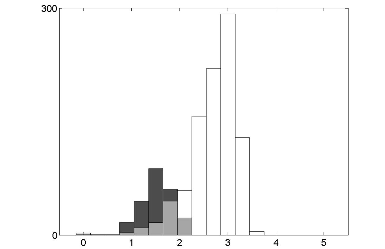
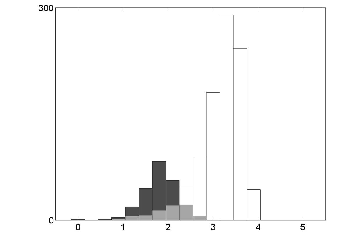
Figure 4. X-Axis: the trust values for the raters. Y-Axis: the density after one iteration (Top), after two iterations (Left), and after convergence (Right). In black: the random raters. In white: the original raters. In grey: both raters.

The reputations are better preserved when using Reputation. It turns out that the reputations given by Reputation take less into account the random users. Moreover, one iteration of the algorithm gives poor information to trust the raters, it is indeed useful to wait until convergence, as seen in Figure 4.

3.2. Robustness against spammers

We now added to the original data set $237$ spammers giving always $1$ except for their preferred movie, which they rated $5$. Let $r^{*}$ and $\tilde{r}^{*}$ be respectively the reputation vector before and after the addition of the random raters. If the reputation vector is calculated according to Reputation, then the $1$-norm difference between $r^{*}$ and $\tilde{r}^{*}$ is

$$\|r^{*}-\tilde{r}^{*}\|_{1}=267,$$

if the reputation vector is the average of the evaluations for each item, then the $1$-norm difference between $r^{*}$ and $\tilde{r}^{*}$ increases:

$$\|r^{*}-\tilde{r}^{*}\|_{1}=638.$$

Figure 5 illustrates this perturbation due to the addition of spammers.

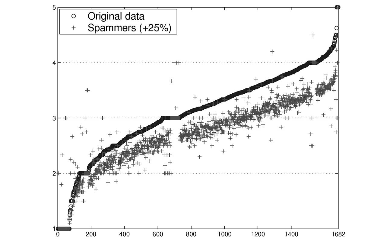
Figure 5. X-Axis: the sorted movies according to their reputations before the addition of spammers. Y-Axis: their reputations according to our algorithm (Top) and to the average (Bottom).

The reputations are again better preserved when using Reputation. Again the reputations given by Reputation take less into account the spammers. As previously, one iteration of the algorithm gives poor information to trust the raters, it is indeed useful to wait until convergence, as seen in Figure 6.

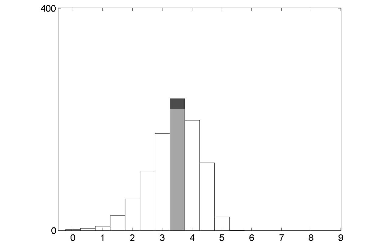
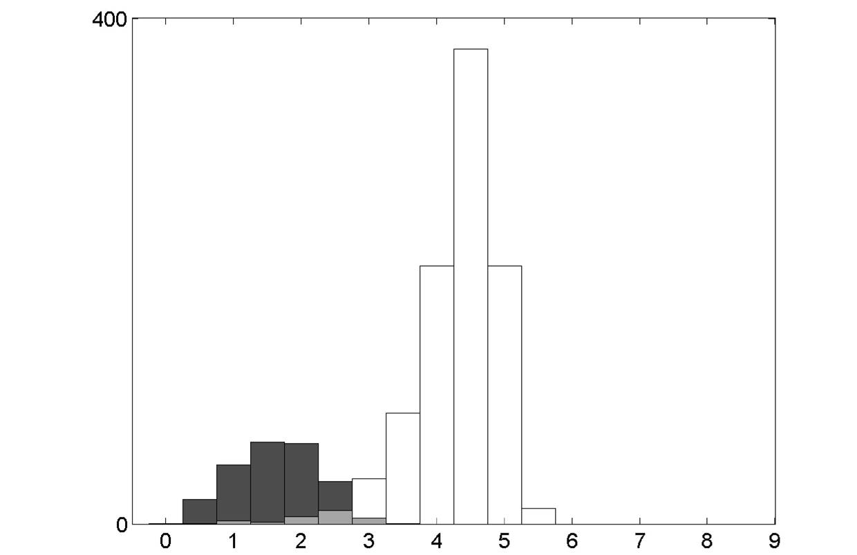
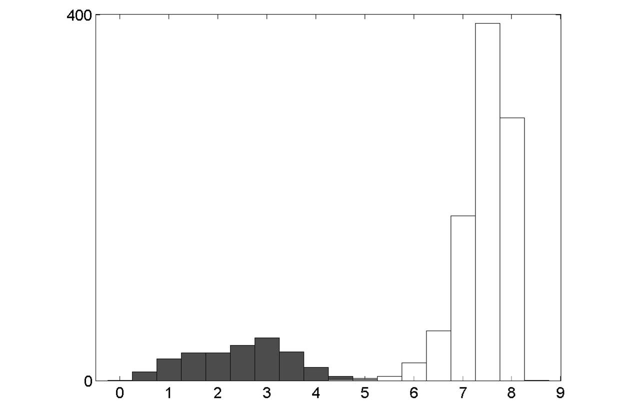
Figure 6. X-Axis: the trust values for the raters. Y-Axis: the density after one iteration (Top), after two iterations (Left), and after convergence (Right). In black: the spammers. In white: the original raters. In grey: both users.

4. Conclusion and Future Work

Our method described in the paper allows us to efficiently refine reputations for evaluated objects from structured data. It is based on the trust we can have in the evaluations of the raters, and also in the raters themselves. The parameters $c_{j}$, introduced in equation 4, make the method flexible, ranging from the average method, i.e. every rater is evenly trusted, until the discriminating method that takes $c_{j}$ as small as possible.

The experiments show interesting results of robustness even though the behavior of the added outliers is somewhat naive. The weights of spammers and random raters are low for the aggregation of the reputation vector. However, other behaviors could be analyzed. For example, clumsy raters could evaluate once correctly and once randomly or we can imagine a more complicated mix of behaviors. Typically, the weights of such raters will be between those of spammers and those of honest raters. Last but not least, the creative cheaters can use engineering to understand the working of the system. The way to proceed is simple: they need to evaluate correctly a group of item and then with that trust, they can rate some target items. In order to significantly change the reputation of these target items, they must have a number of coordinated evaluations larger than the one of honest raters. Therefore such cheaters can easily be disqualified by looking after coordinated ratings to one or several items.

As said at the end of section 2.1, the trust matrix $T$ is the important point for the model. We define it by

$$T_{ij}=c_{j}-d_{i},$$

for any evaluation from $i$ to $j$. Hence, the trust we have in evaluation $T_{ij}$ decreases when the belief divergence $d_{i}$ increases. Other decreasing functions with respect to $d$ make sense. For instance, $T_{ij}=e^{-c_{j}\>d_{i}}$ and $T_{ij}=(c_{j}+d_{i})^{-1}$ may perform well on some data sets. The second definition with $c_{j}=0$ gives the method described in [1]. However, the main difference with our definition lies in the uniqueness of the solution. It turns out that the method in [1] may have several solutions. On the other hand, these solutions can be of interest if they reflect for example two opinion trends.

In section 2.4, the solution is interpreted as the maximizer of the Frobenius norm of $T$. It is possible to maximize other norms of $T$. Then there can be several maximizers and these maximizers will no more satisfy equation (1), but a different one.

We see that our method can be extended towards different directions. Our future work will address the interpretation and the convergence of these extensions.

Acknowledgments.

This paper presents research results of the Belgian Network DYSCO (Dynamical Systems, Control, and Optimization), funded by the Interuniversity Attraction Poles Programme, initiated by the Belgian State, Science Policy Office and supported by the Concerted Research Action (ARC) ”Large Graphs and Networks” of the French Community of Belgium. The scientific responsibility rests with its authors.

References

- [1] P. Laureti, L. Moret, Y.-C. Zhang and Y.-K. Yu, Information Filtering via Iterative Refinement, EuroPhysic Letter 75, pp. 1006-1012, 2006.
- [2] S. Zhang, Y. Ouyang, J. Ford, F. Make, Analysis of a Lowdimensional Linear Model under Recommendation Attacks, Proceedings of the 29th annual International ACM SIGIR conference on Research and development in information retrieval, pp. 517-524, 2006.
- [3] E. Kotsovinos, P. Zerfos, N. M. Piratla, N. Cameron and S. Agarwal, Jiminy: A Scalable Incentive-Based Architecture for Improving Rating Quality, iTrust06, LNCS 3986, pp. 221-236, 2006.
- [4] J. O’Donovan and B. Smyth, Trust in recommender systems, Proceedings of the 10th International Conference on Intelligent User Interfaces, pp. 167-174, 2005.
- [5] L. Page and S. Brin and R. Motwani and T. Winograd, The PageRank Citation Ranking: Bringing Order to the Web, Stanford Digital Library Technologies Project, 1998.
- [6] R. Guha, R. Kumar, P. Raghavan, A. Tomkins, Propagation of Trust and Distrust, Proceedings of the 13th International Conference on World Wide Web, pp. 403-412, 2004.
- [7] G. Akerloff, The Market for Lemons: Quality Uncertainty and the Market Mechanism, Quaterly Journal of Economics, vol. 84 pp. 488-500, 1970.
- [8] S. Kamvar, M. Schlosser and H. Garcia-molina, The Eigentrust Algorithm for Reputation Management in P2P Networks, Proceedings of the 12th International Conference on World Wide Web, pp. 640-651, 2003.
- [9] M. Richardson, R. Agrawal and P. Domingos, Trust Management for the Semantic Web, Proceedings of the 2nd International Conference on the Semantic Web, pp. 351-368, 2003.
- [10] Lik Mui, M. Mohtashemi and A. Halberstadt, A Computational Model of Trust and Reputation, Proceedings of the 35th Annual Hawaii International Conference, pp. 2431-2439, 2002.
- [11] G. Theodorakopoulos and J. Baras, On Trust Models and Trust Evaluation Metrics for Ad Hoc Neworks, Selected Areas in Communications, IEEE Journal on Vol. 24, Issue 2, pp. 318 - 328, 2006.