Tilings of space and superhomogeneous point processes

Abstract

Abstract

We consider the construction of point processes from tilings, with equal volume tiles, of $d$-dimensional Euclidean space $\mathbb{R}^{d}$. We show that one can generate, with simple algorithms ascribing one or more points to each tile, point processes which are “superhomogeneous” (or “hyperuniform”), i.e., for which the structure factor $S({\bf k})$ vanishes when the wavenumber $k$ tends to zero. The exponent of the leading small-$k$ behavior, $S(k\rightarrow 0)\propto k^{\gamma}$, depends in a simple manner on the nature of the correlation properties of the specific tiling and on the conservation of the mass moments of the tiles. Assigning one point to the center of mass of each tile gives the exponent $\gamma=4$ for any tiling in which the shapes and orientations of the tiles are short-range correlated. Smaller exponents, in the range $4-d<\gamma<4$ (and thus always superhomogeneous for $d\leq 4$), may be obtained in the case that the latter quantities have long-range correlations. Assigning more than one point to each tile in an appropriate way, we show that one can obtain arbitrarily higher exponents in both cases. We illustrate our results with explicit constructions using known deterministic tilings, as well as some simple stochastic tilings for which we can calculate $S({\bf k})$ exactly. Our results provide, we believe, the first explicit analytical construction of point processes with $\gamma>4$. Applications to condensed matter physics, and also to cosmology, are briefly discussed.

I Introduction

“Superhomogeneous” Gabrielli et al. (2002) or “hyperuniform” Torquato and Stillinger (2003) point patterns in $d$-dimensional Euclidean space $\mathbb{R}^{d}$ are defined to be those in which infinite wavelength density fluctuations vanish. In other words, the structure factor (or power spectrum) $S({\bf k})$ of the number density field at wave vector $\bf k$ has the following behavior:

$$\lim_{{\bf k}\rightarrow 0}S({\bf k})=0.$$ (1)

This defining characteristic of superhomogeneity (or hyperuniformity) is tantamount to saying that the usual mean-square particle-number fluctuations increases less rapidly than $R^{d}$ for large $R$, where $R$ denotes the linear size of an observation window in $\mathbb{R}^{d}$ Gabrielli et al. (2002); Torquato and Stillinger (2003). Indeed, the magnitude of such local density fluctuations have been suggested as a possible “order metric” to quantify the degree of order (disorder) of an arbitrary point pattern Torquato and Stillinger (2003). Any superhomogeneous point pattern can be seen as a typical configuration of a particular type of “critical” point in that the direct correlation function (defined through the Ornstein-Zernike relation) is long-ranged while the pair correlation function is short-ranged Torquato and Stillinger (2003). Such remarkable behavior is diametric to that seen in usual thermal critical points in which the inverse is true, i.e., the pair correlation is long-ranged and the direct correlation function is short-ranged.

Although it is clear that any periodic point pattern is superhomogeneous, it is less obvious that statistically translationally and even rotationally invariant random point patterns in $\mathbb{R}^{d}$ can have this property. We now know of a variety of intriguing translationally and rotationally invariant random point patterns that are superhomogeneous, including the ground state of liquid ${}^{4}\mbox{He}$ Feynman (1954); Feynman and Cohen (1956); Reatto and Chester (1967), maximally random jammed hard-sphere packings Donev et al. (2005), certain one-component plasmas Baus and Hansen (1980); Gabrielli et al. (2003); Joyce et al. (2005), the matter distribution in the Universe Gabrielli et al. (2002, 2003), and certain aperiodic tilings Gabrielli et al. (2003); Torquato and Stillinger (2003); Hansen et al. (2007). An interesting application of superhomogeneous point patterns in cosmology is in the preparation of initial conditions for gravitational $N$-body simulations Gabrielli et al. (2004a); Gabrielli et al. (2003); Joyce et al. (2005); Hansen et al. (2007). Superhomogeneous distributions also appear in cosmology in the context of the determination of bounds, first derived by Zeldovich Zeldovich (1965), on the mass fluctuations at large scales generated by causal mechanisms (i.e. with physics respecting the causal constraints of cosmological models). Indeed, we note that in this context a simplified form of the analysis we develop here of the small-$k$ behavior of the structure factor is often used (see e.g. Ref. Peebles (1980)).

It is desirable to develop both theoretical and computational methods to generate a wide class of superhomogeneous random point patterns. Recently, a collective coordinate approach Uche et al. (2004, 2006) has been employed to numerically generate translationally invariant superhomogeneous point processes. This procedure enables one to produce point patterns that completely suppress density fluctuations of modes for a positive range of wavenumbers around the origin. In Ref. Gabrielli et al. (2004b) an algorithm for generating discrete processes in one dimension with superhomogeneous mass fluctuations has been given (see also Ref. Fratzl et al. (1991)). An analytical methodology to relate superhomogeneous point processes and Voronoi tilings of space has recently been proposed and studied in Ref. Gabrielli and Torquato (2004).

In this paper, we study the construction of superhomogeneous point patterns starting from generic tilings of Euclidean space $\mathbb{R}^{d}$ with equal volume tiles. We show how to explicitly generate such point processes in which the structure factor for small wavenumbers has the power-law form $S(k)\sim k^{\gamma}$ for positive $\gamma$, where $k\equiv|{\bf k}|$ is the wavenumber. The constructions illustrate the very specific properties of these superhomogeneous point patterns in which the exponent $\gamma$, characterizing the long wavelength fluctuation in $k$ space, is related to the detailed arrangement of the points on small scales. Our study also shows how the exponents of the small-$k$ behavior of the structure factor for these point processes encode properties of the tilings, and could thus possibly be used as a method for classifying them. In a related article by two of us Gabrielli and Joyce the two-point correlation properties of point processes generated by replacing each particle, in a point process with known two point properties, by a “cloud” of particles are derived. One of us Uche et al. (2006) numerically generated disordered point distributions within a cubical box under periodic boundary conditions with $\gamma>4$. However, to our knowledge, prior to this paper and Gabrielli and Joyce , explicit analytical constructions of point processes with $\gamma>4$ have not been given previously in the literature.

It is instructive to recall qualitatively why tilings are a natural starting point for the construction of superhomogeneous point processes. A tiling or tessellation is a partition of Euclidean space $\mathbb{R}^{d}$ into closed regions whose interiors are disjoint regions To02 . Let us suppose we have a tiling of space by tiles which are (i) of equal volume $\|T\|$, and (ii) bounded, with maximal length $\Lambda$ in any direction. Let us now place one point in each tile and consider the number fluctuations in the point process so generated. If $N(R)$ is the number of points in a sphere of radius $R$, and of volume $V(R)$, it is simple to see that

$$\frac{V(R-\Lambda)}{\|T\|}\leq N(R)\leq\frac{V(R+\Lambda)}{\|T\|}\,.$$ (2)

The lower bound is the minimal number of tiles which can overlap the sphere of radius $R-\Lambda$ [and all such tiles must contribute a point to $N(R)$], the upper bound is the maximal number of tiles which are fully enclosed in the sphere of radius $R+\Lambda$ [and only such tiles can contribute to $N(R)$]. For $R\rightarrow\infty$ we have therefore

$$|\Delta N(R)|\leq cR^{d-1}$$ (3)

where $c$ is a constant, and $\Delta N(R)=N(R)-\overline{N}(R)$ with $\overline{N}(R)=V(R)/\|T\|$. Averaging over configurations (or randomly placed centers for the spheres) one anticipates that the slowest possible scaling of number fluctuations is

$$\langle\Delta N^{2}(R)\rangle\propto R^{d-1}$$ (4)

where $\langle...\rangle$ denotes the ensemble (or volume) average. This behavior of the variance, proportional to the surface, is a characteristic of superhomogeneous point processes. If there is appropriate long-range correlation in the tiling at arbitrarily large scale, the fluctuations could however, in principle, add coherently to give the more rapid growth up to

$$\langle\Delta N^{2}(R)\rangle\propto R^{2(d-1)}\,,$$ (5)

which corresponds to the limit equality in Eq. (3). While in $d=1$ this still corresponds to surface fluctuations, for any $d\geq 2$ it implies only the limiting small-$k$ behavior $S(k)\propto k^{\gamma}$ with $\gamma\geq-d+2$, which means that the point processes are not necessarily superhomogeneous for $d\geq 2$. We will recover this result below, with the only difference that the bound is found to be $\gamma>-d+4$, which implies that even long-range correlations between tiles give superhomogeneous processes for $d\leq 4$. The difference between this result and our naive estimate is simply due to the fact that below we constrain the particles to lie at the center of mass, rather than placing them randomly. In fact we will show here that by assigning more than one point in an appropriately constrained manner to each tile, we can increase these bounds on the exponents without limit, and realize superhomogeneous processes with an arbitrary positive exponent, in any dimension.

II Point distributions from tilings: one point per tile

We consider in this section point processes generated by ascribing one point to each tile. We first give a general analysis of the small-$k$ properties of the structure factor of the density fluctuations, and derive how the leading behavior is determined by the properties of the tiling. We then describe some specific explicit constructions which illustrate the result.

II.1 Density fluctuations and long-wavelength limit

We start from a generic (regular or irregular) tiling of $d$-dimensional Euclidean space $\mathbb{R}^{d}$ into equal volume tiles, which we denote $T_{i}$. We consider the point distribution generated by ascribing one point to each tile, and placing it at position xⁱ, which coincides with the center of mass of the tile $T_{i}$, i.e.,

$${\bf x}_{i}=\frac{1}{\|T\|}\int_{T_{i}}d^{d}x\,{\bf x}$$ (6)

where $\|T\|$ is the volume of the tiles. The density fluctuation field is thus

$$\delta n({\bf x})=\sum_{i}\delta^{(d)}\left({\bf x}-{\bf x}_{i}\right)-n_{0}$$ (7)

where $n_{0}$ is the mean number density in the infinite-volume limit, and $\delta^{(d)}({\bf x})$ is the Dirac delta function in $d$ dimensions. The structure factor (SF) is defined as

$$S({\bf k})=\lim_{V\rightarrow\infty}\frac{|\tilde{\delta n}({\bf k};V)|^{2}}{n_{0}V}=1+n_{0}{\tilde{h}}({\bf k})$$ (8)

where $V$ is the system volume,

$$\tilde{\delta n}({\bf k};V)=\int_{V}d^{d}xe^{-i{\bf k}\cdot{\bf x}}\delta n({\bf x})\,,$$ (9)

and

$${\tilde{h}}({\bf k})=\int_{\mathbb{R}^{d}}d^{d}xe^{-i{\bf k}\cdot{\bf x}}h({\bf r})$$ (10)

is the infinite-space Fourier transform of the total pair correlation function $h({\bf r})$, which vanishes for disordered systems when the distance $r\equiv|{\bf r}|$ tends to infinity Torquato and Stillinger (2003); Gabrielli and Torquato (2004).

For our point process it follows directly that

$$\tilde{\delta n}({\bf k};V)=\sum_{i}e^{-i{\bf k}\cdot{\bf x}_{i}}\left[1-\tilde{W_{i}}({\bf k})\right]$$ (11)

where the sum runs over the points enclosed in the volume $V$, and $\tilde{W_{i}}({\bf k})$ is the normalized characteristic function of the tile $T_{i}$, given by

$$\tilde{W_{i}}({\bf k})=\frac{1}{\|T\|}\int_{T_{i}(0)}d^{d}xe^{-i{\bf k}\cdot{\bf x}}\,,$$ (12)

where $T_{i}(0)$ denotes that the center of mass of the tile has been taken as the origin of axes. If we assume that $\tilde{W_{i}}$ is an analytic function at ${\bf k}=0$, we can expand it in Taylor series, to obtain

$$\tilde{W_{i}}({\bf k})=1+\sum_{m=2}^{\infty}\frac{(-i)^{m}}{m!}k_{\alpha_{1}}...k_{\alpha_{m}}M_{\alpha_{1}...\alpha_{m}}(i)$$ (13)

where

$$M_{\alpha_{1}...\alpha_{m}}(i)=\frac{1}{\|T\|}\int_{T_{i}(0)}d^{d}x\,x_{\alpha_{1}}...x_{\alpha_{m}}$$ (14)

is a (fully symmetric) tensor of rank $m$ corresponding to the $m$-th moment of the mass distribution of the tile $T_{i}$ (normalized by the volume/total mass) and $\alpha_{j}=1,\ldots,d$ are indices for the Cartesian components. Note that we have used Eq. (6), which makes the linear term in the expansion (13) (corresponding to the dipole moment) vanish. The assumption of analyticity corresponds to the requirement that all these moments are finite. This is true in particular if the tiles are of finite extent. We will discuss briefly in our conclusions the possibility of relaxing this assumption.

Using these expressions in the definition of $S({\bf k})$ we now obtain

$$S({\bf k})=$$ (15)

$$\sum_{n=2}^{\infty}\sum_{m=2}^{\infty}\frac{(-i)^{m}(i)^{n}}{m!\,n!}k_{\alpha_{1}}...k_{\alpha_{n}}k_{\beta_{1}}...k_{\beta_{m}}{\cal I}_{\alpha_{1}...\alpha_{n}\beta_{1}...\beta_{m}}({\bf k})$$

where

$${\cal I}_{\alpha_{1}...\alpha_{n}\beta_{1}...\beta_{m}}({\bf k})=\lim_{V\rightarrow\infty}\frac{1}{N}\sum_{i}\sum_{j}e^{-i{\bf k}\cdot({\bf x}_{i}-{\bf x}_{j})}$$

$$\times M_{\alpha_{1}...\alpha_{n}}(i)M_{\beta_{1}...\beta_{m}}(j)$$ (16)

where the sums run over the $N$ particles contained in the volume $V$. It is straightforward to verify that the coefficient of the leading term in $k$ (at order $k^{4}$) is non-negative, and that the coefficients of all powers of $k$ are real. Indeed the SF $S({\bf k})$ is by definition a real non-negative quantity, and Eq. (15) is just the specific form of its Taylor expansion around ${\bf k}=0$ for the particular class of distributions we are considering.

It is convenient to rewrite the latter expression as

$${\cal I}_{\alpha_{1}...\alpha_{n}\beta_{1}...\beta_{m}}({\bf k})=\lim_{V\rightarrow\infty}\frac{1}{n_{0}V}\int d^{d}x\,d^{d}y\,e^{-i{\bf k}\cdot({\bf x}-{\bf y})}$$

$${\cal M}_{\alpha_{1}...\alpha_{n}}({\bf x}){\cal M}_{\beta_{1}...\beta_{m}}({\bf y})$$ (17)

where

$${\cal M}_{\alpha_{1}...\alpha_{n}}({\bf x})=\sum_{i}\delta^{(d)}({\bf x}-{\bf x}_{i})M_{\alpha_{1}...\alpha_{n}}(i)\,.$$ (18)

The distribution ${\cal M}({\bf x})$ can be viewed as a weighted particle density. The weight associated with each particle is the appropriate component of the mass moment of the tile to which the particle belongs.

Up to now we have considered implicitly a single particle placed deterministically in each tile. We now consider averaging over an appropriately defined ensemble of such tilings. If the tiling is statistically translationally invariant, we have that

$$\langle{\cal M}_{\alpha_{1}...\alpha_{n}}({\bf x}){\cal M}_{\beta_{1}...\beta_{m}}({\bf y})\rangle\equiv g^{n,m}({\bf x}-{\bf y})\,,$$ (19)

where $\langle...\rangle$ denotes the ensemble average. We have adopted here for the correlation function $g^{n,m}({\bf x})$ the tensorial notation in which the indices are left implicit. In this notation we can write our result for the SF $S({\bf k})$ as

$$S({\bf k})=\frac{1}{n_{0}}\sum_{n=2}^{\infty}\sum_{m=2}^{\infty}\frac{(-i)^{m}(i)^{n}}{m!\,n!}{\bf k}^{n}\cdot\tilde{g}^{n,m}({\bf k})\cdot{\bf k}^{m}$$ (20)

where $\tilde{g}^{n,m}({\bf k})$ is the Fourier transform of $g^{n,m}({\bf x})$ defined as

$$\tilde{g}^{n,m}({\bf k})=\int d^{d}x\,e^{-i{\bf k}\cdot{\bf x}}g^{n,m}({\bf x})\,,$$ (21)

and ${\bf k}^{n}$ denotes a tensor of order $n$, given by the tensor product of $n$ vectors ${\bf k}$, i.e.,

$${\bf k}^{n}_{\alpha_{1}...\alpha_{n}}\equiv[{\bf k}\otimes{\bf k}...\otimes{\bf k}]_{\alpha_{1}...\alpha_{n}}=k_{\alpha_{1}}k_{\alpha_{2}}..k_{\alpha_{n}}\,.$$ (22)

The symbol $\cdot$ in Eq. (20) denotes the contraction of the corresponding tensor indices. If the ensemble is also statistically isotropic the product ${\bf k}^{n}\cdot\tilde{g}^{n,m}({\bf k})\cdot{\bf k}^{m}$, and thus $S({\bf k})$, is a function of $k=|{\bf k}|$ only.

The behavior of $S({\bf k})$ at small $k$ is thus manifestly determined by that of $\tilde{g}^{n,m}({\bf k})$ in this limit. These quantities are in fact the (tensor) SFs associated to the discrete stochastic field defined by Eq. (18), the two point correlation function of which is $g^{n,m}({\bf x})$. They thus encode information about the tiling, and more specifically about the correlation properties of the second and higher moments of the tiles. We restrict ourselves to the case that all these moments are finite, and strictly bounded (which also ensures, as noted above, the validity of the expansion of the characteristic function $\tilde{W_{i}}({\bf k})$ we have performed). As noted above, each component of the tensor stochastic field ${\cal M}^{n}({\bf x})$ defined in Eq. (18) above is then a discrete stochastic process in which the points are located at the same positions as in the point process we are studying, but have “masses” given by the corresponding component of the tensor $M^{n}(i)$ (or rather “charges” as they are not strictly positive) which are bounded (above and below). Just as for a generic stochastic point process such a discrete (or indeed continuous) process can be classified into three categories according to the small-$k$ behavior of the $\tilde{g}^{n,m}({\bf k})$:

1. $\tilde{g}^{n,m}({\bf k}=0)={\rm const.}>0$: this means that the correlation functions $g^{n,m}({\bf x})$ of the higher order moments are integrable at large $x$, and the corresponding integral is equal to a positive constant, i.e., the higher moments of the tiles have short-range correlations dominated by the positive contributions. For the generated point process we have then the leading behavior $S({\bf k}\rightarrow 0)\propto k^{4}$.

2. $\tilde{g}^{n,m}({\bf k}=0)=0$: the integral of the correlation functions $g^{n,m}({\bf x})$ converges to zero, i.e., the shapes and orientations of the tiles have themselves superhomogeneous properties (i.e. in which the positive and negative correlations balance exactly in the integral). In this case we will obtain a leading behavior $S({\bf k}\rightarrow 0)\propto k^{\gamma}$ with $\gamma>4$ [and with a value depending on the leading behavior of the $\tilde{g}^{n,m}({\bf k})$ at small-$k$].

3. $\tilde{g}^{n,m}({\bf k}=0)=\infty$, with $\tilde{g}^{n,m}({\bf k}\rightarrow 0)\propto k^{\alpha}$ and $-d<\alpha<0$. In this case, in which the correlation functions $g^{n,m}({\bf x})$ are non-integrable, i.e., the higher moments of the tiles have themselves long-range correlations, we can obtain a leading behavior for our point process $S({\bf k}\rightarrow 0)\propto k^{\gamma}$ with $4-d<\gamma<4$.

Several remarks on this result are important. Firstly, for simplicity we have assumed above that the $\tilde{g}^{n,m}({\bf k})$ are in the same class for all $m$ and $n$. This is, of course, a priori, not necessarily the case. In the more general case that the different $\tilde{g}^{n,m}({\bf k})$ are in different classes, the determination using Eq. (20) of the exponent $\gamma$ of the leading small-$k$ behavior of $S({\bf k})$ is nevertheless straightforward. Furthermore, it is simple to verify that the bounds we have given on this exponent remain valid.

Secondly, we have assumed that the $\tilde{g}^{n,m}({\bf k})$ obey the condition

$$\lim_{k\rightarrow 0}k^{d}\tilde{g}^{n,m}({\bf k})=0\,.$$ (23)

This assumption corresponds to the requirement that the discrete processes defined by Eq. (18) have well-defined mean values, i.e, the normalized fluctuations (e.g. integrated in a sphere) of the moments of the tiles converge to zero in the infinite-volume limit. While this seems a very weak assumption, it is not a priori true of all tilings.

II.2 Explicit constructions

We now give various explicit constructions to illustrate the above results.

II.2.1 Regular lattice tilings

Consider first the tiling given by the Voronoi cells of any Bravais lattice. In a Bravais lattice, the space $\Re^{d}$ can be geometrically divided into identical regions $F$ called fundamental cells, each of which contains just one point of the lattice. A Voronoi cell associated with a point at ${\bf r}$ in a point distribution is defined to be the region of space nearer to the point at ${\bf r}$ than to any other point. Since all Voronoi cells or tiles of a Bravais lattice have the same shape and orientation, the mass moments $M^{n}(i)$ in Eq. (14), calculated with respect to the center of mass, are identical for all tiles, i.e., $M^{n}(i)$ does not depend on $i$. The discrete processes specified by Eq. (18) are then simply, up to a constant, equal to the density field of the lattice, and thus it follows that all the correlation functions $g^{n,m}({\bf x})$ are proportional to the two point correlation function of the original lattice. Thus $\tilde{g}^{n,m}({\bf k})$, and also $S({\bf k})=0$, is zero in some finite region around ${\bf k}=0$. This result is in fact evident: the point process generated by placing points at the center of mass of every cell is of course simply the lattice itself. In this case, of course, neither the tiling nor the point process are statistically isotropic (where the statistical average is taken over lattices rigidly translated within the elementary lattice cell)

The same result can evidently be generalized to any tiling of equal volume cells constructed from a periodic point pattern.

II.2.2 Congruent rotationally invariant tilings

We consider next deterministic congruent tilings with the additional property of rotational invariance, i.e., in which all orientations of the identical tiles are equiprobable. Known examples are the pinwheel tiling Radin (1995) in $d=2$ (see Fig. 1) and the quaquaversal tiling Conway and Radin (1998) in $d=3$. In these cases each tile $T_{i}$ can be characterized solely by its center of mass ${\bf x}_{i}$ and by a matrix $R(i)\in 0(d)$, the latter giving the orientation with respect to some arbitrary chosen orientation.

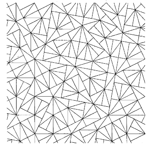
Figure 1: Portion of a pinwheel tiling. The prototile of the pinwheel tiling is a right triangle with sides of length one, two, and $\sqrt{5}$. The tiling is produced by performing certain “decomposition” and “inflation” operations on the prototile. In the first step, the prototile is subdivided into five copies of itself and then these new triangles are expanded to the size of the original triangle. These decomposition and inflation operations are repeated ad infinitum until the triangles completely cover the plane.

We can then write, in tensorial notation,

$${\cal M}^{n}({\bf x})=\sum_{i}\delta^{(d)}({\bf x}-{\bf x}_{i})R^{n}(i)\cdot{\cal\tilde{M}}^{n}$$ (24)

where $R^{n}(i)$ is the tensor product, giving a tensor of rank $2n$ of which $n$ indices are contracted with the corresponding moment ${\cal\tilde{M}}^{n}$ of a tile with the reference orientation, i.e.,

$$[R(i)^{n}\cdot{\cal\tilde{M}}^{n}]_{\alpha_{1}...\alpha_{n}}\equiv R_{\alpha_{1}\beta_{1}}(i)...R_{\alpha_{n}\beta_{n}}(i){\cal\tilde{M}}^{n}_{\beta_{1}...\beta_{n}}$$ (25)

where, as everywhere above, the sums over the indices which appear twice are implicit. The correlation functions $g^{n,m}({\bf x})$ are thus direct measures of the correlation of the orientations of tiles with center of mass separated by ${\bf x}$.

The case of the quaquaversal tiling has been studied numerically in Ref. Hansen et al. (2007), and an approximate small-$k$ behavior $S({\bf k})\propto k^{4}$ found. In Ref. Wang and White it is noted, however, that the numerical results agree better with $S({\bf k})\propto k^{\gamma}$ and $\gamma\approx 3.4$. While the former behavior would correspond, as discussed above, to a short-range correlation of the orientation of the tiles, the latter would instead correspond to a weak long-range correlation (with a correlation function characterizing the orientations decaying with distance $r$ as $\sim r^{-2.4}$). Further, superimposed on this power-law behavior there are residual peaks at certain wavenumbers, with a spacing which appears to be consistent Hansen et al. (2007) with the hierarchical nature of the tiling Radin (1999). As we have discussed the small-$k$ behavior of the constructed point process thus probes the correlation properties of the underlying tiling.

II.2.3 Random Binary Rectangular (RBR) tiling

It is instructive to illustrate our result with a non-trivial example which, albeit not statistically isotropic, allows us to calculate exactly the SF of a point process constructed by the algorithm we have described. The example we now give is of a stochastic congruent tiling. For simplicity we work in $d=2$, but a generalization to any $d$ is straightforward.

We generate the tiling as follows. We start from a regular tiling of the plane with congruent squares. We then divide each square tile in half, defining two identical rectangular sub-tiles, as shown in Fig. 2.

Figure 2: Elementary binary rectangular tiling, with a unit mass particle in the center of mass of each rectangle, and its description in terms of an Ising-like spin variable.

The choice of the orientation of each tile is given by a stochastic process, which can be cast as the value of a simple up-down spin variable. The density of the point process generated using the algorithm analyzed in the previous section, in which a point is placed at the center of mass of each tile, can then be written

$$n({\bf x})=\sum_{{\bf R}}\sum_{n=1}^{2}\delta\left[x-R_{x}-\frac{1+\sigma_{\bf R}}{2}(-1)^{n}\right]$$

$$\times\delta\left[y-R_{y}-\frac{1-\sigma_{\bf R}}{2}(-1)^{n}\right]$$ (26)

where ${\bf R}\equiv(R_{x},R_{y})$ are the lattice sites of the underlying square lattice placed at the center of each square cell, and $\sigma_{\bf R}=\pm 1$ is the spin variable specifying the orientation of the two elementary rectangular tiles at the lattice site ${\bf R}$ as in Fig. 2. We assume that the lattice spacing of the underlying square lattice is $l$. Consequently the volume of the elementary rectangular tile is $l^{2}/2$ and therefore the average number density of the point process is $n_{0}=2/l^{2}$. It is simple to show that the Fourier transform (FT) of $[n({\bf x})-n_{0}]$ is

$$\tilde{\delta n}({\bf k};V)=2\sum_{{\bf R}}e^{-i{\bf k}\cdot{\bf R}}\left[\cos\left(k_{x}l\frac{1+\sigma_{\bf R}}{8}+k_{y}l\frac{1-\sigma_{\bf R}}{8}\right)\right.$$

$$\left.-\frac{\sin(k_{x}l/2)}{k_{x}l/2}\frac{\sin(k_{y}l/2)}{k_{y}l/2}\right]\,.$$ (27)

To calculate the SF averaged over the ensemble of possible configurations of the binary tiles we assume that $\left<\sigma_{\bf R}\right>=0$ (i.e. both orientations of the binary tiles are equiprobable), and write $\chi({\bf R})=\left<\sigma_{{\bf R}_{0}}\sigma_{{\bf R}_{0}+{\bf R}}\right>$ using the lattice statistical translational invariance. Moreover, since $\sigma_{\bf R}=\pm 1$, we have that

$$\cos\left(k_{x}l\frac{1+\sigma_{\bf R}}{8}+k_{y}l\frac{1-\sigma_{\bf R}}{8}\right)$$

$$=\frac{1+\sigma_{\bf R}}{2}\cos\left({k_{x}l\over 4}\right)+\frac{1-\sigma_{\bf R}}{2}\cos\left({k_{y}l\over 4}\right)\,.$$ (28)

It is then straightforward to obtain the following exact expression for the SF:

$$S({\bf k}) = \frac{[\cos(k_{x}l/4)-\cos(k_{y}l/4)]^{2}}{2}\sum_{\bf R}e^{-i{\bf k}\cdot{\bf R}}\chi({\bf R})$$ (29)

$$+ S_{ML}({\bf k})$$

where

$$S_{ML}({\bf k})=A({\bf k})\sum_{\bf R}e^{-i{\bf k}\cdot{\bf R}}=\pi^{2}\sum_{{\bf H}\neq 0}A({\bf H})\delta({\bf k}-{\bf H})$$ (30)

is a “modulated lattice” SF which is different from zero only at the non-zero reciprocal lattice vectors ${\bf H}$, and

$$A({\bf k}) = \frac{1}{2}\left[\cos\left({k_{x}l\over 4}\right)+\cos\left({k_{y}l\over 4}\right)\right.$$ (31)

$$- \left.2\frac{\sin(k_{x}l/2)}{k_{x}l/2}\frac{\sin(k_{y}l/2)}{k_{y}l/2}\right]^{2}\,.$$

At small-$k$ only the first term of Eq. (29) contributes, and expanding the factor outside the sum we thus obtain a leading small-$k$ behavior

$$S({\bf k})\simeq\left({l\over 4}\right)^{4}(k_{x}^{2}-k_{y}^{2})^{2}\tilde{\chi}({\bf k})$$ (32)

where

$$\tilde{\chi}({\bf k})=\lim_{N\rightarrow\infty}\frac{1}{N}\sum_{\bf R}e^{-i{\bf k}\cdot{\bf R}}\chi({\bf R})\,.$$ (33)

This exact result is of course a special case of the general analysis given above, in which the moments characterizing the tiles are particularly simple as there are only two orientations. All the two-point properties of the point process are then contained in the single correlation function $\chi({\bf R})$ of these orientations for pairs of tiles with centers separated by ${\bf R}$. As $\tilde{\chi}({\bf k})$ is a power spectrum of a stochastic process with a well defined mean, at small $k$ we have $\tilde{\chi}(k)\sim k^{b}$ with $b>-d\equiv-2$. If $\tilde{\chi}(0)=c>0$, i.e., in the case in which the orientations of the tiles are short-range correlated, then $S({\bf k})=O(k^{4})$ at small $k$. If instead $\tilde{\chi}(k\rightarrow\infty)=\infty$ there are long-range positive correlations in the orientations of the tiles which induce a slower decay of the fluctuations in the associated point process at large scales. Finally if $\tilde{\chi}(0)=0$ the stochastic spin process is itself superhomogeneous, with a balance between positive and negative correlations creating a sort of “stochastic order” in the spin configuration. In this case $S({\bf k})$ vanishes faster than $k^{4}$ at small $k$. In Appendix A we describe explicitly an algorithm for generating such spin configurations.

III Point distributions from tilings: $n>1$ points per tile

The algorithm described in Sect. II.2.3 can in fact be thought of in a different way to that in which we have presented it: one can consider it instead as a direct assignment of two points to the tiles of the original square lattice, without any construction of an intermediate SBR tiling. The pair of particles then have two possible orientations, which are chosen stochastically. Note that in each case the center of mass of the particles is located at the center of the square cell. Our results above shows that if this stochastic process is short-ranged correlated we obtain a small-$k$ behavior $S(k)\propto k^{4}$, while with a single point at the center of mass of the lattice cell we recovered (evidently) the lattice. We now consider quite generally what small-$k$ behavior of $S(k)$ of a point process we can obtain by ascribing more than one point per tile in a generic tiling with equal volume tiles.

III.1 Density fluctuations and long-wavelength limit

We ascribe $p$ points to each tile, denoting their positions by

$${\bf x}^{i,\ell}={\bf x}^{i}+{\bf u^{i,\ell}}$$ (34)

with $\ell=1...p$ and ${\bf x}^{i}$ is, as above, the center of mass of the tile $T_{i}$ (so that ${\bf u^{i,\ell}}$ is the position relative to the center of mass). We assume further that the center of mass of the points coincides with that of the tile, i.e.,

$$\sum_{\ell=1}^{p}{\bf u^{i,\ell}}=0\,.$$ (35)

Following the same steps as in Sect. II, we arrive at

$$\tilde{\delta n}({\bf k};V)=\sum_{i}e^{-i{\bf k}\cdot{\bf x}^{i}}\left[\frac{1}{p}\sum_{\ell=1}^{p}e^{-i{\bf k}\cdot{\bf u}^{i,\ell}}-\tilde{W_{i}}({\bf k})\right]$$ (36)

where $\tilde{W_{i}}({\bf k})$ is precisely the same normalized characteristic function of the tile as defined in Eq. (12) [and $1/p$ is the fraction of the mass of the tile ascribed to each particle]. Expanding in Taylor series we obtain

$$\frac{1}{p}\sum_{\ell=1}^{p}e^{-i{\bf k}\cdot{\bf u}^{i,\ell}}-W_{i}({\bf k})=\sum_{m=2}^{\infty}\frac{(-i)^{m}}{m!}k_{\alpha_{1}}...k_{\alpha_{m}}M_{\alpha_{1}...\alpha_{m}}(i)$$ (37)

where now

$$M_{\alpha_{1}...\alpha_{m}}(i)=\frac{1}{p}\sum_{\ell=1}^{p}u^{i,\ell}_{\alpha_{1}}...u^{i,\ell}_{\alpha_{m}}-\frac{1}{\|T\|}\int_{T_{i}(0)}d^{d}x\,x_{\alpha_{1}}...x_{\alpha_{m}}$$ (38)

is the totally symmetric rank $m$ tensor corresponding to the difference of the $m$-th moments of the mass distribution of the points associated with the tile $T_{i}$ and that of the tile itself. As in the derivation with one point, we have assumed the analyticity of the quantity we expanded. This means that we require that all the moments in Eq. (38) are finite, which is true in particular if all the tiles are of finite extent and the lengths of the vectors ${\bf u}^{i,\ell}$ are bounded.

All the expressions, and notably the result for $S({\bf k})$ in Eq. (20), derived in the case with one point per tile, are thus valid. The only difference is that the tensors $M^{n}(i)$ [and correspondingly ${\cal M}^{n}({\bf x})$] are now given by Eq. (38). The small-$k$ properties thus depend, assuming statistical translational invariance, on those of the FT of the correlation functions of the differences of the moments of the discrete mass distribution of the points ascribed to each tile and that of the continuous mass distribution represented by the tile itself.

The most important implication of this result is the following: the coefficients in the small-$k$ expansion of Eq. (37) are now proportional to a difference of two quantities in Eq. (38). Any given coefficient will vanish identically if our assignment of the $p$ points satisfies the constraints

$$\frac{1}{p}\sum_{\ell=1}^{p}u^{i,\ell}_{\alpha_{1}}...u^{i,\ell}_{\alpha_{m}}b=\frac{1}{\|T\|}\int_{T_{i}(0)}d^{d}x\,x_{\alpha_{1}}...x_{\alpha_{m}}$$ (39)

in each tile, i.e., if the (tensorial) moments of the mass distribution of the points are equal to those of the tile in which they are placed. With a sufficiently large number of points per tile one can evidently make any desired finite number of terms vanish in the expansion of $S({\bf k})$, i.e., construct a stochastic point mass distribution for each tile which has all moments up to a certain order equal to those of the continuous mass distribution of the tile.

This procedure allows one to obtain an arbitrarily large exponent $\gamma$ in the small-$k$ behavior of the SF of the point process.

III.2 Explicit constructions

We again illustrate these results with some explicit examples.

III.2.1 Regular lattice tiling

In a Bravais lattice, as we have discussed above, the tensorial moments of all tiles are equal so that the second term in Eq. (38) does not contribute to $S({\bf k})$ in a finite region around ${\bf k}=0$. This can most easily be seen by using Eq. (38) directly in the expressions Eqs. (15) and (II.1) for $S({\bf k})$: the $i$-independent second term in each component of the tensor $M^{n}(i)$, when summed over $i$, gives a delta function proportional to the SF of the lattice. If we have more than one point per tile (i.e., $p\geq 2$) we may have, however, an $i$-dependent contribution from the first term in Eq. (38), i.e., from the moments of the mass distribution constituted by the points assigned to the single tile, which are not constrained (beyond the dipole moment). If we allow the distribution of these points to vary stochastically from cell to cell, we will generically have a non-zero contribution for the SF (ensemble averaged over the stochastic process) at all $k$, i.e., we will have a continuous SF.

As a simple example let us consider first the RBR algorithm analyzed above, cast as the ascription of two points to each cell of a simple cubic lattice, but now allowing the pair of particles ascribed to each cubic cell have a random orientation, i.e., we take two points in each lattice cell with coordinates

$${\bf x}_{1}({\bf R})={\bf R}+{\bf u}({\bf R})\,,\qquad{{\bf x}}_{2}({\bf R})={\bf R}-{\bf u}({\bf R})$$ (40)

where ${\bf R}$ is the generic lattice site (which is the center of mass of the corresponding tile), and the vectors ${\bf u}({\bf R})$ are generated by a stochastic process. We assume further that the vectors ${\bf u}({\bf R})$ in different lattice cells are uncorrelated. The ensemble is thus fully specified by the one point probability distribution function $p({\bf u})$. We call this stochastic point process the split shuffled lattice , as it is a generalization of the shuffled lattice discussed in Ref. Gabrielli et al. (2002) (see also Refs. Gabrielli (2004); Gabrielli et al. (2004a)), in which one point is randomly displaced off a perfect lattice.

The leading small-$k$ behavior of $S({\bf k})$ in this case may be found easily by taking the ensemble average of the leading term in Eq. (15):

$$S({\bf k})=\frac{1}{4}k_{\alpha}k_{\beta}k_{\gamma}k_{\delta}\langle{\cal I}_{\alpha\beta\gamma\delta}({\bf k})\rangle$$ (41)

where, using Eq. (38) in Eq. (II.1), we have

$$\langle{\cal I}_{\alpha\beta\gamma\delta}({\bf k})\rangle=\lim_{V\rightarrow\infty}\frac{1}{N}\sum_{{\bf R}}\sum_{{\bf R}^{\prime}}e^{-i{\bf k}\cdot({{\bf R}}-{{\bf R}^{\prime}})}$$

$$\times\langle u_{\alpha}({\bf R})u_{\beta}({\bf R})u_{\gamma}({\bf R}^{\prime})u_{\delta}({\bf R}^{\prime})\rangle\,.$$ (42)

Since the vectors ${\bf u}({\bf R})$ are, by assumption, uncorrelated at different sites, we have

$$\langle u_{\alpha}({\bf R})u_{\beta}({\bf R})u_{\gamma}({\bf R}^{\prime})u_{\delta}({\bf R}^{\prime})\rangle=\langle u_{\alpha}u_{\beta}\rangle\langle u_{\gamma}u_{\delta}\rangle\,.$$ (43)

for ${\bf R}\neq{\bf R}^{\prime}$. Using the fact, again, that the sum $\frac{1}{N}\sum_{{\bf R}}\sum_{{\bf R}^{\prime}}e^{-i{\bf k}\cdot({{\bf R}}-{{\bf R}^{\prime}})}$ is proportional to the SF of the original lattice, which is zero around ${\bf k}=0$, we can then write the leading small-$k$ behavior as

$$S({\bf k})=\frac{1}{4}\left[\langle({\bf k}\cdot{\bf u})^{4}\rangle-\langle({\bf k}\cdot{\bf u})^{2}\rangle^{2}\right]\,.$$ (44)

If we choose a probability distribution which is isotropic in ${{\bf u}}$, i.e., $p({{\bf u}})\equiv p(u)$ (with $u=|{{\bf u}}|)$, we then have

$$S({\bf k})=\frac{k^{4}}{4d^{2}}\left[C(d)\langle u^{4}\rangle-\langle u^{2}\rangle^{2}\right]\,.$$ (45)

where $C(d)\geq 1$ is a constant [$C(1)=1$, $C(3)=9/5$]. We thus obtain the same exponent $\gamma$ as in the RBR tiling model, but now the fluctuations at small $k$ are isotropic at leading order because of the isotropy in the attribution of the displacement vectors. Note that we have assumed here, as we do throughout this paper, that the moments of the mass distribution in each tile are finite, which requires here manifestly in Eq. (45) the finiteness of at least the first four moments of $p(u)$. It is simple, however, to generalize this kind of model to the case when moments of order lower than the fourth diverge, just as done for the shuffled lattice in Ref. Gabrielli (2004) (see also Gabrielli et al. (2004b)). In this case one can obtain any small-$k$ behavior ($0<\gamma\leq 4$).

This kind of algorithm can easily be generalized, conserving a sufficiently large number of moments in such a way as to obtain higher powers of the small-$k$ behavior, in principle producing any desired leading behavior. Let us suppose that we generate mass moments $M^{n}({\bf R})$ at each lattice site ${\bf R}$ defined by Eq. (38), with an uncorrelated stochastic process, i.e., so that

$$\langle M^{n}({\bf R})M^{m}({\bf R}^{\prime})\rangle=\langle M^{n}({\bf R})\rangle\langle M^{m}({\bf R}^{\prime})\rangle$$ (46)

for each tensor component of the tensor product, for ${\bf R}\neq{\bf R}^{\prime}$, (and any $n$, $m$). As in the example given above starting from Eqs. (15) and (II.1), it is straightforward to show that $S({\bf k})$ may then be written, in a finite region around ${\bf k}=0$, as

$$S({\bf k})=\sum_{n=2}^{\infty}\sum_{m=2}^{\infty}\frac{(-i)^{m}(i)^{n}}{m!\,n!}$$ (47)

$$\times{\bf k}^{n}\cdot\left[\langle M^{n}M^{m}\rangle-\langle M^{n}\rangle\langle M^{m}\rangle\right]\cdot{\bf k}^{m}$$

where all the tensors $M^{n}$ are evaluated at the same arbitrary lattice cell, i.e.,

$$[\langle M^{n}M^{m}\rangle]_{\alpha_{1}...\alpha_{n}\beta_{1}...\beta_{m}}\equiv\langle M_{\alpha_{1}...\alpha_{n}}({\bf R})M^{m}_{\beta_{1}...\beta_{m}}({\bf R})\rangle$$ (48)

and $k^{n}\equiv k_{\alpha_{1}}k_{\alpha_{2}}...k_{\alpha_{n}}$ etc..

Thus, for example, we can obtain $\gamma=6$ with an algorithm of this type which allows the third moment $M^{3}$ of the mass distribution to vary from cell to cell while keeping the second (quadrupole) moment $M^{2}$ fixed. This can be done in a rotationally invariant manner by using a configuration of points with a quadrupole moment (relative to its center of mass) proportional to the identity matrix, e.g., points placed at the corners of a regular tetrahedron in $d$ dimensions. Placing such a configuration at each lattice site, but rotated by a random rotation in $SO(d)$, the variance in the second moment of the cell is thus zero. However it is easy to verify that the random rotation engenders a variation in the third moment, so that one obtains the leading small-$k$ behavior $S({\bf k})\propto k^{6}$. The coefficient of the $k^{6}$ term can most easily be made zero by taking instead a configuration whose quadrupole moment is again diagonal, but whose third mass moment $M^{3}$ is zero. Since the latter is in fact zero for any configuration of points which is invariant under inversion symmetry, a possible choice is to add to each tetrahedron a reflection of itself in its center of mass. Alternatively, and using fewer points, one can use a randomly rotated configuration consisting of $d$ couples of points with equal separation placed orthogonally with common center of mass. In this case we obtain a leading order small-$k$ behavior $S({\bf k})\propto k^{8}$. Further discussion of this kind of point process generation can be found in Ref. Gabrielli and Joyce . In this context they arise as a special case of “cloud processes”, in which points in a generic initial point process, of which the correlation properties are assumed known, are replaced by a “cloud” of point particles.

III.2.2 Congruent rotationally invariant tilings

We have seen that superhomogeneous point processes with a small-$k$ behavior $S({\bf k})\propto k^{\gamma}$ and $\gamma>4$ can be generated starting from a regular lattice tiling, by using a stochastic process to determine the positions of an appropriately constrained set of points in each cell. While the point process so generated is not statistically translationally and rotationally invariant, we saw that a leading behavior proportional to $k$ was obtained if the stochastic process assigning the points had itself no preferred direction. Thus at large scales the system approximates very well statistical translational and rotational invariance.

Starting from a translation and rotation invariant tiling we can obtain a statistically translation and rotation invariant point process in an analogous way. It suffices in this case, however, to assign the points deterministically to each tile, in the same way relative to each tile (e.g. at the center of mass of the tile). We do not need now the additional stochasticity provided either by taking more points per tile or random positions inside the tile. The reason is that the moments of the tiles given by Eq. (14) already depend on the tile itself because of the orientation. Consequently the quantities $\tilde{g}^{n,m}({\bf k})$ are non-zero around ${\bf k}=0$ just as in the case when we had one point per tile. The difference is, as we have discussed at length above, that we can make certain terms zero so that the leading term appears at higher order in $k$.

To see how this can be done in a little more detail, let us consider, to be specific, a pinwheel tiling ($d=2$) or quaquaversal tiling ($d=3$) as in Sect. II.2.2 above. It is convenient to study the SF $S({\bf k})$ as given in Eq. (20), where now the $M^{n}$ in Eq. (14) are given by the expressions in Eq. (38). To define a point distribution in which the leading term in this expression vanishes, one can proceed as follows. First one determines the location of the center of mass and the quadrupole moment of the elementary tile. From the latter one can then find the principal axes, in which it is diagonal. In each tile of the tiling one then places on each such axis a pair of points, with their center of mass at that of the tile, at the appropriate distance to produce the component of the second moment along the corresponding axis. The leading contribution to $S({\bf k})$ should then be determined by the small-$k$ behavior of $\tilde{g}^{3,3}({\bf k})$, i.e., by the correlation properties of the third moment $M^{3}$ as in Eq. (38). Because of the inversion symmetry in the point distribution in each tile, the first term in Eq. (38) vanishes. It is therefore the correlation properties of the third moment of the tiles alone which determines the coefficient of the term at order $k^{6}$. Given the results discussed above of the numerical studies Hansen et al. (2007) for the quaquaversal tiling with a single point at the center of mass, we expect that such correlations are short-range, or at most very weakly long-range. One would expect therefore to obtain an $S(k)\propto k^{\gamma}$ with $\gamma\approx 6$.

The generalization of this algorithm to higher orders is, in principle, straightforward (albeit evidently cumbersome as the order increases). Further one can seek to determine the minimal number of points per tile required to make the desired number of terms in Eq. (20) vanish. Indeed the specific algorithm described above uses $2d$ points, while it is easy to see that one needs only a smaller number to make the leading term in Eq. (20) vanish: in $d=2$, for example, it suffices to have three (rather than four) points to represent the quadrupole moment of the elementary triangular tile of the pinwheel tiling.

IV Discussion and conclusions

We have studied a class of point processes generated by placing one or more points in each tile of a tiling of $\mathbb{R}^{d}$. We have assumed that the tiles have equal volume as this is expected to lead to the suppression of fluctuations at large scales characteristic of superhomogeneous point processes. We have shown explicitly that one can build superhomogeneous point processes with an arbitrarily large exponent characterizing the small-$k$ behavior of the structure factor, and we have presented various examples. To our knowledge exact constructions of such point processes for the case $\gamma>4$ have not previously been given in the literature.

We have shown how in these algorithms the exponent $\gamma$ depends (i) on the arrangements of the points ascribed to the tiles in the algorithm, and (ii) on the correlation properties of the shapes and orientations of the tiles. For the specific case of regular lattice tilings a non-trivial contribution to the small-$k$ behavior of $S({\bf k})$ arises only from the former, with the coefficients in the small-$k$ expansion depending explicitly only on the variance of the (tensorial) mass moments of the points assigned to each cell. By arranging a sufficient number of points in a way which makes this variance zero for the first $n$ moments, one can obtain $\gamma>2n$. In the case of an irregular tiling — we have considered the example of pinwheel and quaquaversal tilings — an identical arrangement of the points in each tile can be sufficient to produce continuous SF and translational and rotational invariant superhomogeneous point processes. The exponent $\gamma$ then encodes information about the correlation properties of the shapes and orientations of the tiles. If these are short-range correlated, one obtains $\gamma=4$ placing a single point at the center of mass of each tile, and $\gamma=2(n+1)$ if one places a number of points with all mass moments up to the $n$-th equal to that of the elementary tile. If there is, on the hand, long-range correlation in the shapes and orientations of tiles, the exponent obtained will be modified in a way which depends on the nature of this correlation.

Our results shed light on the meaning of the exponent $\gamma>0$ characterizing a superhomogeneous point process. Up to the value $\gamma=4$ previous explicit constructions of discrete processes (see, e.g., Gabrielli (2004); Gabrielli et al. (2004b)) have shown that the increase of $\gamma$ can be associated with a suppression of fluctuations at large scales. Here we have seen that values $\gamma>4$ correspond indeed to an increased order in the arrangement of the points, but now at small scales: it is by changing how points are arranged within each tile, i.e., below a finite length scale (but subject always to the global constraints on fluctuations imposed by the tiling), that we can increase the exponent. Thus to “undo” the order represented by an exponent $\gamma>4$ with respect to a system with $\gamma=4$ requires only the rearrangement of the system at small scales, while to “undo” that in a system with $\gamma\leq 4$ require a coherent rearrangement of points on arbitrarily large scales (i.e. on scales inverse to the wavenumber range in which the exponent is measured).

We have mentioned that our results are relevant in cosmology. Firstly the analysis given here makes more rigorous certain heuristic arguments used in this context regarding “causal constraints” on the generation of fluctuations from a uniform background Zeldovich (1965); Peebles (1980). An algorithm like that described here, for the case of a single point placed at the center of mass of each tile, has been considered Peebles (1980) as a toy model for the generation of fluctuations starting from an exactly uniform mass density, by a physical process which conserves mass and momentum locally. The result $\gamma=4$ is obtained by assuming that space is divided into finite cells whose positions are uncorrelated. The latter assumption is in fact not consistent: the division of space into equal volume cells implies that their positions are necessarily correlated. Our more rigorous analysis shows that this exponent $\gamma=4$ does result generically, however, if the shapes and orientations of these cells (i.e. tiles) are short-range correlated, i.e., have integrable correlation functions.

Secondly, the generation of very uniform point processes is of relevance to the generation of initial conditions for numerical simulations of structure formation in the universe. In this context, to represent a given set of initial conditions, one must perturb appropriately (see Joyce and Marcos (2007) for a detailed discussion) a point distribution representing as well as possible the uniform (unperturbed) universe. To understand the effects coming from this chosen point distribution (which are non-physical) it is desirable to have different algorithms which can generate such configurations. It is for this reason that a special case of the algorithm we have studied here has been built explicitly and studied numerically in this context Hansen et al. (2007). The analytical results we have given here complement these studies and give further algorithms for producing even more uniform point processes which may be useful in this context. We note again in this respect that explicit algorithms for producing $\gamma>4$ have not previously been given. Such distributions in themselves provide interesting initial conditions (without any perturbation) for gravitational clustering, which have not previously been studied.

We conclude with some further remarks on our results and some other directions for further work:

• In our constructions of point processes we have always constrained the center of mass of the points in each tile to coincide with that of the tile. We have done so because our goal here has been to generate point processes which are as uniform as possible. It is a simple exercise to redo our calculation leading to Eqs. (15) and (II.1) when this constraint is relaxed, i.e., allowing the center of mass of the particles (or particle) in each tile to be displaced randomly from that of the tile. The result is that the leading term in Eqs. (15) is now at order $k^{2}$ rather than $k^{4}$. For short-range correlated tilings the leading behavior of the SF will then be proportional to $k^{2}$. This result will be valid if the displacements of the center of mass of the particles within a tile with respect to the center of mass of the associated tiles have a finite variance. On the other hand, if the variance of these displacements diverges, the small-$k$ behavior of the SF is given by $S({\bf k})\propto k^{\gamma}$ where $0<\gamma<2$, the value of the exponent depending on the precise behavior displacements PDF for large arguments. A detailed calculation of these cases for a randomly perturbed lattice can be found in Ref. Gabrielli (2004); Gabrielli et al. (2004a).

• While we have shown analytically the existence of point processes with arbitrarily large exponents $\gamma$, we have not done so for a case which is statistically translation and rotation invariant. In the latter case our results for the exponent are expressed in terms of the small-$k$ behavior of the ${\tilde{g}}^{n,m}({\bf k})$ which encode, as we have explained, information about the correlation properties of the shapes and orientations of the tiles. For the one such example which has been numerically studied (in Ref. Hansen et al. (2007), the quaquaversal tiling with a single point at the center of mass) the result indicates an asymptotic behavior close to (but, as noted in Ref. Wang and White , slightly different to) that which would arise from a purely short-range correlation of the orientations of the tiles. Further numerical and analytical study of these points processes would clearly be of interest, in particular of the simpler pinwheel tiling.

• We have made in our derivations here an assumption of analyticity at ${\bf k}=0$ of the window function of the tiles, which corresponds to all moments of their mass distribution being finite. This is certainly valid if the tiles are of finite extent. It may, however, include other cases which might be of interest, e.g., in $d>1$ one may envisage that there is a non-trivial distribution of the shapes of the equal volume tiles, in which the extent of a tile is not limited. One could also consider relaxing the assumption that the volumes of the tiles are strictly equal, admitting a distribution of volumes with specified correlation properties. In analogy with what has been found in certain algorithms for $\gamma\leq 4$ Gabrielli (2004); Gabrielli et al. (2004b), one would expect that such modifications would allow the generation of point processes with leading non-analytic behavior, and any value of the exponent $\gamma$. Indeed one would expect non-analytic exponents to be related either to the divergence of moments of such a distribution of extent or volume or to the presence of long-range tile-tile correlations.

• While all our explicit examples have employed tilings which are congruent, our results for the small-$k$ behavior of the SF $S({\bf k})$ all apply only on the much weaker assumption of equal volume of the tiles. Thus for example we can apply these results to any tiling generated by a deformation of tiles which leaves their volume fixed, which could encompass a large range of systems of physical interest (cells, foams, etc.). We recall in this respect, as remarked above, that a point placed randomly in each cell, rather than at the center of mass, leads to the restoration of the order $k^{2}$ term in the expression given in Eqs. (15).

• It is useful to briefly remark on the physical realizability of superhomogeneous point distributions with arbitrary positive but bounded values of $\gamma$. Such distributions are disordered to some degree and, although they are unusual, can be physically constructed. For example, the maximally random jammed (MRJ) state in three dimensions To00 is a special disordered sphere packing that can be regarded to be a prototypical glass because it is perfectly rigid and yet is maximally disordered. It is a superhomogeneous point distribution characterized by an exponent $\gamma=1$ Donev et al. (2005), but it is inherently a system out of equilibrium. While we have examples like the equilibrium one-component plasma that has $\gamma=2$, can one devise equlibrium superhomogeneous point distributions in which $\gamma$ is arbitrarily large? The answer is apparently in the affirmative but it requires more than just pair interactions, namely, two-, three- and four-body interactions as shown in Ref. Uche et al. (2004).

MJ and AG thank ST for hospitality at Princeton University during a visit in May 2006. MJ thanks B. Jancovici and J. Lebowitz for useful discussions. ST gratefully acknowledges the support of the Office of Basic Energy Sciences, DOE, under Grant No. DE-FG02-04ER46108.

Appendix A From Gaussian to spin fields

In this appendix we show explicitly how to generate a regular lattice spin configuration with a given two-point correlation function. Such a configuration has been used as the starting point in the RBR algorithm described in Sect. II.2.3.

The algorithm we propose is based on a mapping between a set of correlated Gaussian variables $\{x({\bf R})\}$ with zero mean, and the spin set $\{s({\bf R})\}$ (where ${\bf R}$ is, as above, the generic lattice vector). We do so because to generate a lattice set of correlated Gaussian variables with any possible desired correlation function is very simple.

We denote by

$$c({\bf R})=\left<x({\bf R}_{0})x({\bf R}_{0}+{\bf R})\right>$$ (49)

and

$$\chi({\bf R})=\left<s({\bf R}_{0})s({\bf R}_{0}+{\bf R})\right>$$

the two-point correlation functions of the Gaussian and the spin sets, respectively. We have used here the statistical lattice translational invariance. Both $c({\bf R})$ and $\chi({\bf R})$ must have non-negative FTs as required by the Khintchine theorem for stochastic processes (see e.g. Ref. Gabrielli et al. (2004a)).

The starting point is the two variable joint PDF for correlated and monovariate Gaussian variables. Denoting by $x_{1}$ and $x_{2}$ two Gaussian variables at two lattice sites separated by the vector ${\bf R}$, we have

$$p(x_{1},x_{2};{\bf R}) =\frac{1}{2\sqrt{\sigma^{4}-c^{2}({\bf R})}}$$ (50)

$$\times\exp\left[-\frac{\sigma^{2}(x_{1}^{2}+x_{2}^{2}-2c({\bf R})x_{1}x_{2}}{2[\sigma^{4}-c^{2}({\bf R})]}\right]\,,$$

where $c({\bf R})$ is defined in Eq. (49), and $\sigma^{2}=c(0)$ is the common variance of the Gaussian variables.

The mapping we consider is the simplest possible: at the site ${\bf R}$ we fix $s({\bf R})=1$ if $x({\bf R})>0$ and $s({\bf R})=-1$ otherwise. We want now to find the relation between $\chi({\bf R})$ and $c({\bf R})$. This can be done simply by noting that we can write

$$s({\bf R})=2\theta[x({\bf R})]-1\,,$$

where $\theta(x)$ is the usual Heaviside step function. Therefore we can write

$$\chi({\bf R}) =4\int_{0}^{+\infty}\int_{0}^{+\infty}\frac{dx_{1}\,dx_{2}}{2\sqrt{\sigma^{4}-c^{2}({\bf R})}}$$ (51)

$$\times\exp\left[-\frac{\sigma^{2}(x_{1}^{2}+x_{2}^{2}-2c({\bf R})x_{1}x_{2}}{2[\sigma^{4}-c^{2}({\bf R})]}\right]-1\,.$$

Performing the double change of integration variables

$$\left\{\begin{array}[]{l}y_{1}=x_{1}\\ y_{1}=x_{2}-[c({\bf R})/\sigma^{2}]x_{1}\end{array}\right\}$$

it is simple to rewrite Eq. (51) as

$$\chi({\bf R})=2\int_{0}^{\infty}\frac{dy_{1}}{\sqrt{2\pi\sigma^{2}}}e^{-y_{1}^{2}/(2\sigma^{2})}\mbox{erf}(Ay_{1})\,,$$ (52)

where $A=\frac{c({\bf R})}{\sigma\sqrt{2[\sigma^{4}-c^{2}({\bf R})]}}$ and

$$\mbox{erf}(x)=\frac{2}{\sqrt{\pi}}\int_{0}^{x}dt\,e^{-t^{2}}$$

is the usual error function. We now use the known equality:

$$\int_{0}^{\infty}dx\,e^{-px^{2}}\mbox{erf}(qx)=\frac{1}{\sqrt{\pi p}}\mbox{arctg}\left({a\over\sqrt{p}}\right)$$

which implies finally that

$$\chi({\bf R})=\frac{2}{\pi}\mbox{arctg}\left[\frac{c({\bf R})}{\sqrt{\sigma^{4}-c^{2}({\bf R})}}\right]\,.$$ (53)

Therefore, given a lattice set of monovariate correlated Gaussian variables, we can map it onto a lattice set of spin variables with $\left<s({\bf R})\right>=0$ and $\chi({\bf R})$ given by Eq. (53).

A.1 Asymptotics

From Eq. (53) it is simple to verify that

$$\chi(0)=\left<\sigma^{2}\right>=1\,.$$

Moreover, as for $R=|{\bf R}|\to\infty$ the correlation function $c({\bf R})$ must vanish, it is simple to verify that for sufficiently large $R$ we have

$$\chi({\bf R})\simeq{2\over\pi}{c({\bf R})\over\sigma^{2}}$$

, i.e., $\chi({\bf R})$ and $c({\bf R})$ have the same asymptotic behavior. In particular if the Gaussian variables are long-/short-range correlated the spin variables are also long-/short-range correlated with the same scaling behavior.

We can also give the condition of superhomogeneity for the spin lattice set. For the spin system this condition is simply

$$\sum_{{\bf R}}\chi({\bf R})=0\,.$$

which gives the following more complicated relation for the correlation function of the Gaussian variables:

$$\sum_{{\bf R}}\frac{2}{\pi}\mbox{arctg}\left[\frac{c({\bf R})}{\sqrt{\sigma^{4}-c^{2}({\bf R})}}\right]=0\,.$$

References

- Gabrielli et al. (2002) A. Gabrielli, M. Joyce, and F. Sylos Labini, Phys. Rev. D 65, 083523 (2002).
- Torquato and Stillinger (2003) S. Torquato and F. H. Stillinger, Phys. Rev. E68, 041113 (2003), publisher’s note: Phys. Rev. E, 68, 069901 (2003). Note that the horizontal axis of Fig. 9 in this paper is mislabeled: should be .
- Feynman (1954) R. P. Feynman, Phys. Rev. 94, 262 (1954).
- Feynman and Cohen (1956) R. P. Feynman and M. Cohen, Phys. Rev. 102, 1189 (1956).
- Reatto and Chester (1967) L. Reatto and G. Chester, Phys. Rev. 155, 88 (1967).
- Donev et al. (2005) A. Donev, F. Stillinger, and S. Torquato, Phys. Rev. Lett. 95, 090604 (2005).
- Baus and Hansen (1980) M. Baus and J.-P. Hansen, Physics Reports 59, 1 (1980).
- Gabrielli et al. (2003) A. Gabrielli, B. Jancovici, M. Joyce, J. L. Lebowitz, L. Pietronero, and F. Sylos Labini, Phys. Rev. D67, 043506 (2003).
- Joyce et al. (2005) M. Joyce, D. Levesque, and B. Marcos, Phys. Rev. D72, 103509 (2005).
- Hansen et al. (2007) S. Hansen, O. Agertz, M. Joyce, J. Stadel, B. Moore, and D. Potter, Astrophys.J. 656, 631 (2007), eprint astro-ph/0606148.
- Gabrielli et al. (2004a) A. Gabrielli, F. Sylos Labini, M. Joyce, and L. Pietronero, Statistical Physics for Cosmic Structures (Springer, 2004a).
- Zeldovich (1965) Y. B. Zeldovich, Adv. Astron. 3, 241 (1965).
- Peebles (1980) P. J. E. Peebles, The Large-Scale Structure of the Universe (Princeton University Press, 1980).
- Uche et al. (2004) O. Uche, F. H. Stillinger, and S. Torquato, Phys. Rev. E70, 046112 (2004).
- Uche et al. (2006) O. Uche, S. Torquato, and F. H. Stillinger, Phys. Rev. E74, 031104 (2006).
- Gabrielli et al. (2004b) A. Gabrielli, M. Joyce, B. Marcos, and P. Viot, Europhys. Lett. 66, 1 (2004b), eprint astro-ph/0303169.
- Fratzl et al. (1991) P. Fratzl, J. Lebowitz, O. Penrose, and J. Amar, Phys. Rev. B44, 4794 (1991).
- Gabrielli and Torquato (2004) A. Gabrielli and S. Torquato, Phys. Rev. E70, 041105 (2004).
- (19) A. Gabrielli and M. Joyce, Two point correlation properties of stochastic cloud processes, eprint arXiv:0711.0270.
- (20) S. Torquato, Random Heterogeneous Materials: Microstructure and Macroscopic Properties (Springer-Verlag, New York, 2002).
- Radin (1995) C. Radin, Notices Amer. Math. Soc. 42, 26 (1995).
- Conway and Radin (1998) J. Conway and C. Radin, Inventiones Math. 132, 179 (1998).
- (23) J. Wang and S. White, Discreteness effects in simulations of hot/warm dark matter, astro-ph/0702575.
- Radin (1999) C. Radin, J. Stat. Phys. 95, 827 (1999).
- Robinson and Wandelt (1996) J. Robinson and B. Wandelt, Phys. Rev. D53, 618 (1996), eprint astro-ph/9507043.
- Gabrielli (2004) A. Gabrielli, Phys. Rev. E70, 066131 (2004), eprint cond-mat/0409594.
- Joyce and Marcos (2007) M. Joyce and B. Marcos, Phys. Rev. D75, 063516 (2007), eprint astro-ph/0410451.
- (28) S. Torquato, T. M. Truskett, and P. G. Debenedetti, Phys. Rev. Lett. 84, 2064 (2000).