A Large Sky Simulation of the Gravitational Lensing of the Cosmic Microwave Background
Abstract
Large scale structure deflects cosmic microwave background (CMB) photons. Since large angular scales in the large scale structure contribute significantly to the gravitational lensing effect, a realistic simulation of CMB lensing requires a sufficiently large sky area. We describe simulations that include these effects, and present both effective and multiple plane ray-tracing versions of the algorithm, which employs spherical harmonic space and does not use the flat sky approximation. We simulate lensed CMB maps with an angular resolution of . The angular power spectrum of the simulated sky agrees well with analytical predictions. Maps generated in this manner are a useful tool for the analysis and interpretation of upcoming CMB experiments such as PLANCK and ACT.
Subject headings:
cosmic microwave background — gravitational lensing — large-scale structure of universe — methods: N-body simulations — methods: numerical1. Introduction
While the current generation of CMB experiments have had a significant impact on cosmology by helping to establish a standard paradigm for cosmology (Spergel et al., 2003, 2007), the upcoming generation of CMB experiments still has the potential to provide novel new insights into cosmology. PLANCK111http://www.rssd.esa.int/index.php?project=Planck and ground based experiments, such as the Atacama Cosmology Telescope (ACT)222http://www.physics.princeton.edu/act, will be mapping the CMB sky with significantly higher angular resolution than ever before. Secondary anisotropies on small angular scales encode important information about the late time interaction of CMB photons with structure in the Universe. One of the most basic of these interactions is the gravitational effect of the large scale structure potentials deflecting the paths of the photons, an effect justifiably referred to as the Gravitational Lensing of the CMB.
The effect of gravitational lensing can be thought of as a remapping of the unlensed CMB field by a line-of-sight averaged deflection field (for a recent review, see Lewis & Challinor, 2006). Therefore, lensing does not change the one-point properties of the CMB. However, it does modify the two and higher-point statistics, and generates non-Gaussianity (Seljak, 1996; Zaldarriaga & Seljak, 1999; Zaldarriaga, 2000). Although the typical deflection suffered by a CMB photon during its cosmic journey is about three arcminutes, the deflections themselves are coherent over several degrees, which is comparable to the typical size of the acoustic features on the CMB. Thus lensing causes coherent distortions of the hot and cold spots on the CMB, and thereby broadens their size distribution. This leads to redistribution of power among the acoustic scales in the CMB, and shows up in the two-point statistics as a smoothing of the acoustic peaks. At smaller scales, where the primordial CMB is well approximated by a local gradient, deflectors of small angular size produce small-scale distortions in the CMB, thereby transferring power from large scales in the CMB to the higher multipoles. Also, although the primordial CMB can be safely assumed to be a Gaussian random field (Komatsu et al., 2003), and the large scale lensing potential can also be well approximated by a Gaussian random field, the lensed CMB— being a reprocessing of one Gaussian random field by another— is itself not Gaussian. The effect of lensing on the power spectrum of the CMB is important enough that it should be taken into account while deriving parameter constraints with future higher resolution experiments. But what is even more interesting is that the non-Gaussianity in the lensed CMB field should enable us to extract information about the projected large scale structure potential, and thereby constrain the late time evolution of the Universe and Dark Energy properties. Therein lies the main motivation of studying this effect in utmost detail. Progress in this area has been slow. Measurements of the CMB precise enough to enable a detection of weak lensing were not available in the pre-WMAP era. Also, picking out non-Gaussian signatures in the measured CMB sky by itself is extremely difficult, due to confusion from systematics, foregrounds, and limited angular resolution.
Rather than looking at signatures of lensing only in the CMB, one can also measure to what extent the deflection field estimated from the CMB correlates with tracers of the large scale structure which contributed to the lensing. It is easily realized that this approach is powerful (Peiris & Spergel, 2000) because many of the systematics disappear upon cross-correlating data sets. This approach was taken in recent years by Hirata et al. (2004) and Smith et al. (2007), using WMAP 1-year and 3-year data respectively. The former work looked at the cross correlation with SDSS luminous red galaxies (LRG), while the latter used the NRAO-VLA Sky Survey (NVSS) radio sources as their large scale structure tracers. As the lensing efficiency for the CMB is highest between redshifts of one and four, higher redshift tracers should show greater cross correlation signal, which makes the NVSS radio sources better tracers for such study; Smith et al. (2007) report a detection. An independent analysis by Hirata et al. (2008) looking for this effect in the WMAP 3-year data in cross correlation with SDSS LRG+QSO and NVSS sources find this signal at the level. With these pioneering efforts and with higher resolution CMB data from experiments such as ACT, PLANCK and the South Pole Telescope (SPT)333http://spt.uchicago.edu on the horizon, we are entering an era where robust detection and characterization of this effect will become a reality. Also, with upcoming and proposed large scale structure projects (LSST444http://www.lsst.org/lsst_home.shtml, SNAP555http://snap.lbl.gov/, ADEPT666http://universe.nasa.gov/program/probes/adept.html, DESTINY777http://destiny.asu.edu/, etc.) there will in future be many more datasets to cross-correlate with the CMB.
One of the immediate results of such cross-correlation studies will be a measurement of the bias of the tracer population. Because such cross correlations tie together early universe physics from the CMB and late time evolution from large scale structure, they will also be sensitive to Dark Energy parameters (Hu et al., 2006) and neutrino properties (Smith et al., 2006a; Lesgourgues et al., 2006), and can potentially break several parameter degeneracies in the primordial CMB (M. Santolini, S. Das and D. N. Spergel, in preparation). Combination of galaxy or cluster lensing of the CMB with shear measurements from weak lensing of galaxies can also provide important constraints on the geometry of the Universe (S. Das and D. N. Spergel, in prep; Hu et al., 2007). Again, with high enough precision of CMB data, it is possible to estimate, using quadratic (Okamoto & Hu, 2003) or maximum likelihood (Hirata & Seljak, 2003) estimators, the deflection field that caused the lensing. Such estimates can be turned into strong constraints of the power spectrum of the projected lensing potential (Hu & Okamoto, 2002), which is also sensitive to the details of growth of structure. The estimated potential from the lensed CMB alone, or the potential estimated from weak lensing surveys (Marian & Bernstein, 2007), can be also used to significantly de-lens the CMB. This is particularly important in the detection of primordial tensor modes via measurements of CMB polarization. This is because (even though detection of the so-called B modes in CMB polarization is hailed as the definitive indicator of the presence of gravitational waves from the inflationary era) these mode can be potentially contaminated by the conversion of E-modes into B-modes via gravitational lensing. De-lensing provides a way of cleaning these contaminating B-modes produced by lensing and thereby probing the true gravitational wave signature.
In this paper, we describe a method for simulating the gravitational lensing of the CMB temperature field on a large area of the sky using a high resolution Tree-Particle-Mesh (TPM; Bode et al., 2000; Bode & Ostriker, 2003) simulation of large scale structure to produce the lensing potential. The reason for considering a large area of the sky is twofold. First, the deflection field has most of its power on large scales (the power spectrum of the deflection field peaks at in the best-fit cosmological model), and much of the power redistribution in the acoustic peaks of the CMB occurs via coupling of modes in the CMB with these large coherent modes in the deflection field. A large sky allows for several such modes to be realized. It is estimated that a small (flat) sky simulation that misses these modes would typically underestimate the lensing effect by about in the acoustic regime, and more in the damping tail (Hu, 2000). Second, one of the major goals of simulations such as this is to produce mock observations for upcoming CMB experiments. PLANCK is an all-sky experiment, and many of the future CMB experiments (including ACT and SPT) will observe relatively large patches of the sky. Therefore, simulating CMB fields on a large area of the sky is a necessity. This method fully takes into account the curvature of the sky. Although presented here for a polar cap like area, it can be trivially extended to the full sky.
The value of a simulation as described here is multifaceted, particularly in the development of algorithms for detection and characterization of the CMB lensing effect for a specific experiment. Since each experiment has a unique scanning mode, beam pattern, area coverage, and foregrounds, operations and optimizations performed on the data to extract the lensing information will have to be tailored to the specific experiment. A large-sky lensed CMB map acting as an input for a telescope simulator provides the flexibility of exploring various observing strategies, and also allows for superposition of known foregrounds. Another important aspect of this simulation is that the halos identified in the large scale structure simulation can be populated with different tracers of interest. Also, other signals, such as the Thermal and Kinetic Sunyaev Zel’dovich effects and weak lensing of galaxies by large scale structure, can be simulated using the same large scale structure. This opens up the possibility of studying the cross-correlation of the CMB lensing signal with various indicators of mass, and thereby predicting the level of scientific impact that a specific combination of experiments can have.
As noted in Lewis (2005), the exact simulation of the lensed CMB sky, which requires the computation of spin spherical harmonics on an irregular grid defined by the original positions of the photons on the CMB surface, is computationally expensive and requires robust parallelization. Lewis (2005) suggested an alternative in which one would resample an unlensed CMB sky, generated with finer pixelation, at these unlensed positions. This method was implemented in the publicly available LensPix888http://cosmologist.info/lenspix code that was based on Lewis (2005). However, producing a high resolution lensed map requires a much higher resolution unlensed map, the generation of which becomes computationally more expensive as resolution increases. Here we put forward another alternative, in which we do the resampling with a combination of fast spherical harmonic transform on a regular grid followed by a high order polynomial interpolation. This interpolation scheme has been adapted from Hirata et al. (2004), and is called the Non-Isolatitude Spherical Harmonic Transform (NISHT). This method is accurate as well as fast, and does not require parallelization or production of maps at a higher resolution. Another added advantage of this method is that the same algorithm can be used to generate the gradient of a scalar field on an irregular grid. Since the deflection field is a gradient of the lensing potential, this opens up the possibility of performing a multiple plane ray tracing simulation. This is because the rays, as they propagate from one plane to another, end up on irregular grids, so the deflection fields on the subsequent planes have to be evaluated on irregular grids. At the time of the development of this project, LensPix did not include an interpolation scheme, and used the methods as described originally in that paper. Concurrently with the completing of the current work, an interpolation scheme (Akima, 1996) different from the one described here has been added to that code. Another notable difference of our results with LensPix, is that while the latter uses a Gaussian Random realization of the deflection field, we have used a large scale structure simulation to produce the same, thereby including all higher order correlations due to non-linearities.
The paper is laid out as follows. In §2 we explain the lensing algorithm, describing the governing equations in §2.1 and their discretization in §2.2. Then we discuss the effective lensing approach (§2.3) as well as the multiple plane ray tracing approach (§2.4). At the heart of the lensing algorithm lies the non-isolatitude spherical harmonic transform algorithm adapted from Hirata et al. (2004), which is reproduced in some detail for completeness in §2.5. As discussed earlier, we have employed a light cone -body simulation and adopted a special polar cap like geometry for generating the lensing planes (§3). For comparison of the simulated fields with theoretical prediction, we compute the angular power spectra on the polar cap window; in §4 we describe some of the subtleties involved in computing the power spectra. We present our results in §5 and describe the tests that we have performed in §6. Conclusions are presented in §7.
2. The Lensing Algorithm
2.1. Basic Equations
We would like to note here that while the calculations for the simulation described here has been done for a flat universe, our approach is generalizable to non-flat geometries.
The deflection angle of a light ray propagating through the space is
| (1) |
where is is the deflection angle, is the Newtonian potential, denotes the spatial gradient on a plane perpendicular to light propagation direction and is the radial comoving distance. The transverse shift of the light ray position at due to a deflection at is given by
| (2) |
where is the comoving angular diameter distance.
The final angular position is therefore given by
| (3) | |||||
where is the total effective deflection.
2.2. Discretization
We will now discretize the above equations by dividing the radial interval between the observer and the source into concentric shells each of comoving thickness . We project the matter in the -th shell onto a spherical sheet at comoving distance which is halfway between the the edges of the shell ( increases as one moves away from the observer). Since we shall be working in spherical coordinates it is advantageous to use angular differential operators instead of spatial ones. We rewrite equation 1 in terms of the angular gradient as
| (4) |
At the -th shell at , the deflection angle due to the matter in the shell can be approximated by an integral of the above:
| (5) | |||||
| (6) |
where we have defined the 2-D potential on the sphere as
| (7) |
Here, the notation signifies that the potential is evaluated at the conformal look-back time , when the photon was at the position . The potential can be related to the mass overdensity in the shell via Poisson’s equation, which reads
| (8) |
being the mean matter density of the universe at redshift . By integrating the above equation along the line of sight, one can arrive at a two dimensional version of the Poisson equation (Vale & White, 2003),
| (9) |
where the surface mass density
| (10) |
Note that in going from the three dimensional to the two dimensional version, the term containing the radial derivatives of the Laplacian can be neglected (Jain et al., 2000). One can show that this term is small by expanding the potential in Fourier modes , with components parallel to the line of sight and transverse to it. Then, the ratio of the components of the line of sight integral in the parallel and transverse directions will be . Due to cancellation along the line of sight, only the modes with wavelengths comparable to the line of sight depth of each slice will survive the radial integral. These would be the modes with . On the other hand, the transverse component gets most of its contribution from scales smaller than Mpc i.e. Mpc-1. Under the effective lensing approximation, the projection is along the entire line of sight from zero redshift to the last scattering surface, Mpc, giving Mpc-1. Therefore, in this case the ratio of the radial and transverse components of the integral will be . For a multiple plane case, we would typically employ lensing planes for which this ratio would be . The approximation will break down if we employ thin shells.
Defining the field as
| (11) |
equation 9 takes the form
| (12) |
It is convenient to define an angular surface mass density as the mass per steradian,
| (13) |
The surface mass density defined in equation 10 is related to this through the relation
| (14) |
This implies the following form of equation 11,
| (15) |
Equation (15) is the key equation here. The quantity can be readily calculated once the mass density is radially projected onto the spherical sheet. Expanding both sides of equation 12 in spherical harmonics, one has the following relation between the components:
| (16) |
It is interesting to note that the apparently divergent monopole modes in the lensing potential can be safely set to zero in all calculations, because a monopole term in the lensing potential does not contribute to the deflection field. Being the transverse gradient of the potential, the deflection angle is a vector (spin 1) field defined on the sphere and can be synthesized from the spherical harmonic components of the potential in terms of vector spherical harmonics, as will be described in § 2.5.
2.3. Connection with effective lensing quantities

In weak lensing calculations, one often takes an effective approach, in which one approximates the effect of deflectors along the entire line of sight by a projected potential or a convergence which is computed along a fiducial undeflected ray (often referred to as the Born approximation). One therefore defines an effective lensing potential out to comoving distance as
| (17) |
In terms of the projected potential, the effective deflection (see Eq. 3) is given by the angular gradient, . An effective convergence is also defined in a similar manner:
| (18) | |||||
In terms of the fields and defined on the multiple planes, these quantities are immediately identified as the following sums,
| (19) | |||
| (20) |
Once is obtained one can go through the analog of equation (16) and take its transverse gradient to obtain the effective deflection . Using this, one can find the source position corresponding to the observed position :
| (21) |
In §5, we shall use this effective or single plane approximation to lens the CMB.
Equation (21) is to be interpreted in the following manner (Challinor & Chon, 2002). The effective deflection angle is a tangent vector at the undeflected position of the ray. The original position of the ray on the source, or unlensed, plane is to be found by moving along a geodesic on the sphere in the direction of the tangent vector and covering a length of an arc. The correct remapping equations can be easily derived from identities of spherical triangles (Lewis, 2005). For completeness, we give the derivation here.
In Fig. 1, let the initial and final position of the ray in question be the points A and B, respectively. The North pole of the sphere is indicated as C, so that the dihedral angle at A is also the angle between and , so that
| (22) |
Now, applying the spherical cosine rule to the triangle ABC, we have
| (23) |
and applying the sine rule
| (24) |
We use these equations to remap points on the CMB sky and on the intermediate spherical shells in the multiple plane case, as described below.
2.4. Multiple plane ray tracing

In the multiple plane case, we shoot ray outwards from the common center of the spherical shell (i.e. the observer) and follow their trajectories out to the CMB plane, thereby studying the time reversed version of the actual phenomenon. We assume all intermediate deflections are small, as is really the case. Here we describe how we keep track of a ray propagating between multiple planes, as shown in Fig. 2. We assume a flat cosmology for this purpose. At some intermediate stage of the ray propagation, let a ray be incident on the -th plane at the point A, where it gets deflected and reaches the +1-th plane at the point D. The ray incident at A will not in general lie on the same plane as defined by the deflected ray and the center O of the sphere, which we also consider as the plane of the figure. Assuming that we know the incidence angle , we can obtain the additional angle of deflection due to the matter on plane and compute the net deflection . Let us denote by , the effective angle, by which a ray has to be remapped from its observed position to its current position on plane i, so that
| (25) |
Obviously, and . Therefore, the effective angle by which the ray has to be remapped from point B to point D on the shell +1 can be readily calculated from two descriptions of the arc BD,
| (26) |
In order to repeat this process for the (+2)-th shell, one needs to know the value of the new incidence angle . We now equate two ways of finding the length of the arc AC,
| (27) |
Substituting from equation 26,
| (28) |
Since we shoot the rays radially on the first plane, ; therefore equations (26) and (28) can be used to propagate the ray back to the CMB surface, which we take to be the -th plane, i.e. . Although we only discuss results obtained with the effective or single plane approximation here, the multiple plane version is straightforward to perform and will be reported elsewhere.
2.5. Interpolation on the sphere
In practice we have used the HEALPix 999http://healpix.jpl.nasa.gov (Gorski et al., 2005) scheme to represent fields on the sphere. At various stages of the lensing calculation, an accurate algorithm for interpolation on the sphere becomes a necessity. In the effective lensing approximation, the original positions of the rays will in general be off pixel centers. This implies that the lensed CMB field is essentially generated by sampling the unlensed CMB surface at points which are usually not pixel centers. Hence, obtaining the lensed CMB field is essentially an interpolation operation. In the case of multiple lensing planes, it is again obvious that (except for the first plane, on which we can shoot rays at pixel centers by way of convenience) the deflection field itself has to be evaluated at off-center points on all subsequent planes. So, together with the interpolation of the temperature map. we need to go between spin-0 and spin-1 fields on an arbitrary grid. Therefore, one needs, in general, a spherical harmonic transform algorithm that can deal with an irregular grid on the sphere.
For this purpose, we adopt the Non-isolatitude Spherical Harmonic Transform (NISHT) algorithm proposed by Hirata et al. (2004); details of the algorithm can be found in Appendix A of that paper. Here we have reproduced the key equations for clarity, and described the salient features of the general algorithm with special attention to aspects which are relevant for the current application.
The basic operation for generating the lensed CMB maps can be broken
up into two steps:
L1. generating the deflection field on the sphere at
points where the rays land from the previous plane, and
L2. sampling the unlensed CMB surface at the source-plane
positions of the rays to generate the lensed CMB field.
Of course, in case of the effective lensing simulation, one can conveniently generate the deflection field at the pixel centers in step L1 above. As step L2 is a series of operations involving scalars and therefore conceptually simpler, we shall explain the NISHT algorithm in relation to this step. Step L1, which involves spin-1 fields on the sphere, is conceptually similar to the spin-0 case.
The problem in step L2 is that we know the CMB temperature field on the HEALPix grid as well as the source-plane positions of the rays on the polar cap, and we want to sample the CMB field at . Suppose, by applying the steps for spherical harmonic analysis (as will be described later), we have the spherical harmonic components, of the temperature field. Now, we need to synthesize the field using these ’s at the points . This operation can be formally written as
| (29) |
where is the Nyquist multipole and is set by the resolution of the HEALPix grid as, (cf. equation 40). This synthesis operation can be split into the following four steps (Eqns. 30 through 35 are essentially reproduced for completeness from Appendix A of Hirata et al. 2004):
-
1.
Coarse Grid Latitude Transform
As the first step, we perform a transform in the latitude direction on an equally spaced set of points, , where is an integer in the range and is a small integral multiple of some power of two such that :(30) The above calculation involves operations.
-
2.
Refinement of Latitude Grid
In this step we reduce the grid spacing from to where . We take advantage of the fact the sampling theorem can be applied to a linear combination of spherical harmonics which is band limited in the multipole space, and hence can be written as a Fourier sum,(31) We determine the coefficients via a fast Fourier Transform (FFT) of length and evaluate using an inverse FFT of length . This step saves us the expensive generation of Associated Legendre Polynomials on the finer grid. Each FFT requires operations.
-
3.
Projection onto Equicylindrical Grid
Next, we perform the standard SHT step of taking an FFT in the longitudinal direction to generate ,(32) After this step we have synthesized the map on an Equicylindrical projection (ECP) grid. The operation count for this step is and the total operation count including this step is .
-
4.
Interpolation onto the final grid
In the final step, given a required position , we find the nearest grid point in the ECP grid and determine the fractional offset, between the two points,(33) Then we perform a two dimensional polynomial interpolation using points around the nearest grid point, obtaining the value at the required point as
(34) with the weights computed using Lagrange’s interpolation formula,
(35)
The inverse of the synthesis operation described above is the analysis operation, in which the spherical harmonic coefficients of a map defined on an irregular grid is needed. This can be thought of as the transpose of the above operations applied in reverse, and hence can be accomplished in an equal number of steps.
The above algorithm can be easily extended to deal with vector and tensor fields on the sphere. For a vector (spin 1) field, the natural basis of expansion are the vector spherical harmonics,
| (36) |
where the superscripts and represent the “vector-like” and the “axial-vector-like” components, respectively. In terms of these a vector field can be expanded as,
| (37) |
Therefore, given the () components one can go through the analogs of the above steps for the scalar field synthesis. In fact, to accomplish step L1 of the lensing algorithm, we go from the convergence field to the deflection field,
| (38) | |||||
Therefore, we go from the field on the polar cap to the spherical harmonic components using the analysis algorithm for scalar fields; then we divide the result by . This defines the vector field harmonic components as from which we synthesize the deflection field at the required points.
The accuracy of the interpolation can be controlled by two parameters: the rate at which the finer grid oversamples the field i.e. the ratio , and the order of the polynomial used for the interpolation. Increasing either of these increases the accuracy. In this paper we have used and , which yields a fractional interpolation accuracy per Fourier mode of .
3. Generation of the lensing planes
An -body dark matter simulation was performed to generate the large scale structure; this same simulation has been discussed in Sehgal et al. (2007) and Bode et al. (2007), so we refer the reader to these papers for more details. Briefly, a spatially flat CDM cosmology was used, with a total matter density parameter and vacuum energy density . The scalar spectral index of the primordial power spectrum was set to and the linear amplitude normalized to . The present day value of the Hubble parameter . A periodic box of size was used with particles; therefore the particle mass was . The cubic spline softening length was set to 16.28 .
3.1. From the box to the sphere
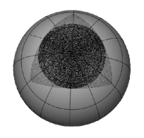
We create the lensing planes on-the-fly from the -body simulation. At each large time step (set by a Courant condition such that no particle moves more than kpc in this time) the positions and velocities of the particles in a thin shell are saved. The mean radius of the shell is the comoving distance to the redshift at that time, and the width (a few ) corresponds to the time step. Each shell is centered on the origin of the simulation and covers one octant of the sky (). Note that for shells with radii greater than the simulation box size, periodic copies of the box are used. Thus a given structure will appear more than once in the full light cone, albeit at different times and viewed from different angles. We then Euler rotate the coordinate axes so that the new -axis passes through the centroid of the octant. This is done to make the centroid correspond to the North Pole on the HEALPix sphere. We use the HEALPix routine vec2pix to find the pixel that contains the particle’s position on the sky. We then place the mass of the particle into that pixel by assigning to it the surface mass density , where is the area of a pixel in steradians (cf. equation 40). Thus, if particles fall inside the beam defined by a pixel, then the pixel ends up having a surface mass density of . To simplify the geometry, we save only those particles which fall inside a Polar Cap like region defined by the disc of maximum radius that can be cut out from the octant (see Fig. 3).
By the end of the run, such planes were produced from the simulation, spanning to . As these are far too many planes for the purpose of lensing, we reduce them into planes by dividing up the original planes into roughly equal comoving distance bins and adding up the surface mass density pixel by pixel for all planes that fall inside a bin to yield a single plane per bin. Hereafter, we shall refer to the original planes from the TPM run as the TPM-planes and the small number of planes constructed by projecting them as the lensing-planes.
The angular radius of the Polar Cap is given by , and the solid angle subtended by it is . Due to pixelation, the true total area of the pixels that make up the Polar Cap is not exactly equal to , but rather
| (39) |
We will denote the surface mass density in pixel as which has units of mass per steradian.
In HEALPix , the resolution is controlled by the parameter NSIDE, which determines the number, of equal area pixels into which the entire sphere is pixelated, through the relation , so that the area of each pixel becomes,
| (40) |
The angular resolution is often expressed through the number . It is also useful to define the fraction area of the sphere covered by the polar cap as,
| (41) |
For results presented in this paper the resolution parameter NSIDE was set to , which corresponds to an angular resolution of .
3.2. From surface density to convergence
To construct the quantities required for lensing, we first convert the surface mass density maps into surface over-density maps as defined in equation 14. It is straightforward to obtain the -maps defined in equation 15 from the above map. Finally, equation 20 is used to obtain the effective convergence map on the Polar Cap. It is evident that the convergence map constructed out of the simulated lensing planes in this way will only contain the contribution from large scale structure up to the redshift of the farthest lensing plane (). However, to accurately lens the CMB we need to add in the contribution from higher redshifts up to the last scattering surface. We do this by generating a Gaussian random field from a theoretical power spectrum of the convergence between and , computed from the matter power spectrum obtained using CAMB, and adding it onto the convergence map from the TPM simulation.
3.3. The unlensed CMB map
We used the synfast facility in HEALPix to generate the unlensed CMB map. This takes as an input a theoretical unlensed power spectrum and synthesizes a Gaussian-random realization of the unlensed CMB field. For computing the theoretical power spectrum we have used the publicly available Boltzmann transfer code CAMB111111http://www.camb.info, with the same set of cosmological parameters as used for the large scale structure simulation.
4. Measuring Angular Power Spectra
At several stages we compute the power spectra of the maps to compare with theory. For example, to verify that we have created the convergence map correctly, the angular power spectrum of the map is computed and compared to the theory. Also, we do the same for the lensed map on the polar cap. We use the map2alm facility of HEALPix to perform a spherical harmonic decomposition of a map on the Polar Cap. The resulting spherical harmonic components, i.e. ’s, are then combined to obtain the pseudo-power spectrum,
| (42) |
There are two effects that need to be taken into account before comparing the above result with theory, namely the finite pixel size, signified by the superscript, and the incomplete sky coverage, represented by the tilde.
To simplify the following discussion of pixelation effects, for the moment we shall ignore the effect of the incomplete sky coverage. Also, we shall use the shorthand notation to denote the sum . Due to the finite pixel size, a field realized on the HEALPix sphere is a smoothed version of the true underlying field, i.e. the value of the field in pixel is given by
| (43) |
where is the window function of the -th pixel as is given by
| (44) |
Expanding the true field in terms of spherical harmonics as
we have
| (45) |
where
| (46) |
is the spherical harmonic transform of the pixel window function. In the HEALPix scheme, due to the azimuthal variation of the pixel shapes over the sky, especially in the polar cap area, a complete analysis would require the computation of these coefficients for each and every pixel. However, even for a moderate NSIDE, this calculation becomes computationally unfeasible. Therefore, it is customary to ignore the azimuthal variation and rewrite equation 46 as
| (47) |
where one defines an azimuthally averaged window function
| (48) |
From equations (47) and (45) it immediately follows that the estimate of the power spectrum of the pixelated field is given by
| (49) |
where one defines the pixel averaged window function,
| (50) |
This function is available for NSIDE in the HEALPix distribution. We take out the effect of the pixel window by dividing the computed power spectrum by the square of the above function. Coming back to the case at hand, where we have both pixel and incomplete sky effects, we recover the power spectrum after correcting for the pixel window function in this manner.
The second and more important effect that one needs to take into account results from the fact that our field is defined only inside the polar cap. This is equivalent to multiplying a full sky map with a mask which has value unity inside the polar cap and zero outside. As is well known, such a mask leads to a coupling between various multipoles, leading to a power spectrum which is biased away from the true value. As this effect tends to move power across multipoles, the problem is more acute for highly colored power spectra like the CMB.
Let us denote the effective all-sky mask with , where
| (51) |
The spherical harmonic components of the masked field is therefore given by
| (52) | |||||
| (53) |
and the measured power spectrum by (see for example Hivon et al., 2002)
| (54) | |||||
where is the true power spectrum and is the mode coupling matrix given by
| (55) |
with the power spectrum of the mask defined as
| (56) |
being the spherical harmonic components of the mask .
For a polar cap with angular radius , this function is analytically known to be (Dahlen & Simons, 2007)
| (57) |
where is a Legendre Polynomial of order and

The window function in equation 51 corresponding to the polar cap is a “tophat” in the sense that it abruptly falls to zero at the edge. The power spectrum (equation 57) of this window has an oscillatory behavior showing a lot of power over a large range of multipoles, an effect sometimes called ringing. Ringing causes the mode coupling matrix, to develop large off-diagonal terms, as illustrated in Fig. 4, and consequently the value of the measured power spectrum at any multipole (equation 54) has non-trivial contributions from many neighboring multipoles. This causes the measured power spectrum to be biased, and its effect is particularly evident for power spectra with a sharp fall-off such as the CMB. As is evident from Fig. 4, the effect of mode coupling due to the polar cap becomes a serious problem for the lensed and unlensed power spectra starting at moderately low multipoles (). Although in principle one could compare the measured power spectrum with a theoretical power spectrum which has been convolved with the same mode coupling matrix, the effect is so strong in this case that the lensed and unlensed spectra almost overlap each other. This problem can be mitigated in principle by inverting a binned version of the mode coupling matrix and thereby decorrelating the power spectra. However an easier and less computationally expensive solution can be achieved in the following manner.
The off diagonal terms of the mode coupling matrix can be reduced significantly by apodizing the polar cap window function. Parenthetically, we note that there exists a general method of generating tapers on a cut-sky map, so as to minimize the effect of mode coupling. This is referred to as the multi-taper method (S. Das, A. Hajian and D. N. Spergel, 2007, in preparation; Dahlen & Simons, 2007). However, for our purpose, it suffices to define a simpler apodizing window as
| (58) |
The power spectrum of this window can be easily computed using HEALPix , and thus the mode coupling matrix can be readily generated using equation 55. We found that an apodization window with degree, corresponding to pixels, works extremely well without eating into too much of the map. A section of the mode coupling matrix and the corresponding convolved power spectrum are displayed in Fig. 4. This figure shows that the power spectrum convolved with the apodized window function has negligible mode coupling. Parenthetically, it is interesting to note that simply scaling the theory power spectrum by the fraction of the sky covered, , seems to do a good job in mimicking the effect of the partial sky coverage, at least for the lower multipoles. In fact, this approximation is an exact result for a white power spectrum. However, when the window is apodized, the effective area of coverage, , goes down a little (by for our apodization). We use scaled theory power spectra only in some plots in this paper. For the analysis, we perform the full mode coupling calculation. Therefore, when comparing the power spectrum of some quantity defined on the polar cap with theoretical predictions, we first multiply the map by the apodized window and compare the resulting power spectrum with the theoretical power spectrum mode-coupled through the same weighting window.
5. Results
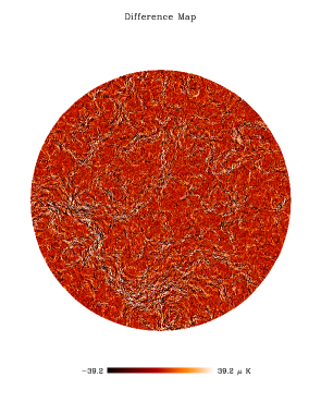
We illustrate the algorithm with an effective lensing simulation at the HEALPix resolution of . Since some rays end up outside the polar cap after lensing, we have actually used an unlensed CMB realization (using the synfast facility of HEALPix ) on an area larger than our fiducial polar cap to accommodate those rays. As the gradient of the lensing potential is ill defined at the edge of the polar cap, we ignore a ring of pixels near the edge of the lensed map for all subsequent analyses. It is particularly instructive to look at the difference of the lensed and the unlensed maps, as shown in Fig. 5, as it shows the large scale correlations imprinted on the CMB due to the large scale modes in the deflection field.
We compute the angular power spectrum of the lensed and unlensed CMB maps using an apodized weighting scheme as discussed in §4. The resulting power spectra are displayed in Fig. 6 for the entire range of multipoles analyzed, and are compared with the mode-coupled theoretical power spectra. The theoretical lensed CMB power spectrum used for the calculation was generated with the CAMB code, using the all-sky correlation function technique (Challinor & Lewis, 2005) and including nonlinear corrections to the matter power spectrum. In Fig. 7, we show a zoomed-in version of the lensed power spectrum, in the multipole range . From visual inspection of these plots it is evident that the simulation does a good job in reproducing the theoretically expected lensed power spectrum, at least in the range of multipoles over which the computation of the theoretical power spectrum is robust. We defer a detailed comparison of the simulation to the theory to §6.3.


6. Tests
6.1. Tests for the mass sheets
In this section we perform some sanity checks to ensure that the projection from the simulation box onto the Polar Cap has been properly performed. We first test that the total mass in each slice is equal to the theoretical mass expected from the mean cosmology, the later being given by
| (59) |
where is the comoving thickness of the slice at a comoving distance . We compare this quantity with
| (60) |
which is the total mass on the plane from the simulation. The percentage difference between the two is depicted in Fig. 8 for the lensing-planes. Notice that the agreement is good to within 0.5% for the high redshift planes, in which the solid angle corresponds to a large comoving area. For low redshifts there are large variations due to the fact that matter is highly clustered and corresponds to a small comoving area. These fluctuations at low redshift represent the chance inclusion or exclusion of large dark matter halos within the light cone.

Next, we make sure that the probability density function (PDF) of the surface mass density is well behaved for each plane, and is well modeled by analytic PDFs such as the lognormal (Kayo et al., 2001; Taruya et al., 2002) or the model proposed by Das & Ostriker (2006). In Fig. 9 we show these two models over-plotted on the PDFs drawn from the forty-five lensing-planes.
The model of Das & Ostriker (2006) is a better fit to the simulation than the lognormal, especially at high surface mass density. Note in that paper the authors used the first year WMAP parameters, whereas the present simulation is run with the WMAP 3-year parameters, including a significantly different . The fact that the model still represents the simulation well suggests that it is quite general.

6.2. Tests for the convergence plane
As described in §3.2, the effective convergence plane was produced by a two step process. First, we computed the effective convergence plane by weighting the surface mass density planes from the simulation with appropriate geometrical factors. Let us call it the map . This map, therefore, includes contribution from the large scale structure only out to the redshift of the farthest TPM plane, . Next we added in the contribution from , by generating a Gaussian random realization of the effective convergence from a theoretical power spectrum (the map ). Therefore the final convergence map is simply . It is interesting to compare the power spectrum of the map with that expected from theoretical considerations. Since CMB lensing is most sensitive to large scale modes, we should make sure that these modes were realized correctly in our simulated convergence plane. Incidentally, these scales are also linear to mildly nonlinear. Therefore, we should expect the power spectrum of the convergence map to be well replicated by the theoretical prediction at least in the quasi-linear range of multipoles () where simple non-linear prescriptions suffice.
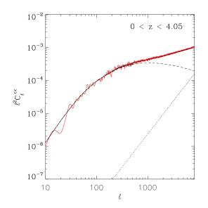
In order to compute the theoretical power spectra for the maps and , we used the Limber approximation to project the matter power spectrum computed from CAMB. The Limber approximation simplifies the full curved-sky calculation, and is valid for . Since for lower values of the multipole we have few realizations of the convergence modes, the power spectrum computed from the simulated map is noisy in this regime, rendering it practically useless for comparison with theory. Therefore, an accurate computation of the theoretical convergence power spectrum for these lowest multipoles is unnecessary, and the Limber calculation suffices. Under the same approximation, the shot noise contribution to the convergence field can be computed as
| (61) |
where , being the total number of particles in the -th shell.
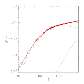
We compute both a linear and a non-linear version of the convergence power spectrum, where the latter includes non-linear corrections to the matter power spectrum from a halo model based fitting formula (Smith et al., 2003). We plot the power spectrum computed from the simulated convergence map , and the corresponding theoretical power spectra, in Fig. 10. As is evident from the figure, the simulated power spectrum is in accord with the linear theory power spectrum for , beyond which the effect non-linearities creep in. However, it is impressive that the non-linear corrections to the power spectrum are in good agreement with the simulation up to relatively high multipoles. The same quantities are plotted for the convergence map out to the redshift of the CMB in Fig. 11. We find in both cases that beyond multipoles of the simulation contains more non-linear power than predicted by the theory.
6.3. Tests for the lensed CMB map
Since CMB lensing is essentially a remapping of points, the one-point statistics should remain unaffected by the lensing. We check for this by drawing up the one-point PDF’s of the unlensed and lensed maps, and find them to be consistent to within . Next, we compare the power spectrum of the simulated lensed map (cf. Figures 6 & 7) with the theoretical predictions as computed with the CAMB code. For a quantitative comparison, we consider a range of multipoles in the acoustic regime. We do not consider the lower multipoles as they exhibit negligible lensing effect. We found that for a fixed input cosmology, the tail () of the lensed CMB power spectrum predicted by CAMB depends somewhat sensitively on input parameters, specifically the combination , which controls the maximum value of the wavenumber for which the matter power spectrum in computed. However, the lensed power spectrum from CAMB is robust towards changes in the auxiliary input parameters for the range of multipoles, . Also, the lensed CMB multipoles beyond this range couple to relatively small scale modes of the deflection field where our simulation has more power than expected from non-linear theory. In fact, beyond the simulated power spectrum is found to deviate systematically from the theoretical spectrum.
As the simulated power spectrum, , was computed using an apodized window as described in §4, the appropriate theoretical curve to compare this result with is the power spectrum from CAMB after it has been convolved with the coupling matrix defined by the same weighting scheme (cf. equation 54 ). We denote the latter quantity by . In order to facilitate the comparison we bin the raw spectrum in . In the multipole range considered , the quantity is flat (see Fig. 7) and therefore a better candidate for binning. We denote the difference between the simulated and the theoretical version of this quantity by
| (62) |
For each of the bins indexed by , we compute the mean, , and the sample variance, , of the observations falling inside that bin. In order to account for that fact that cosmic variance errors will be higher in our case due to incomplete sky coverage, we define an effective variance as .

We quantify the goodness of fit between the simulation and the model by defining a statistic as
| (63) |
We perform the analysis by uniformly binning the power spectra in the range into bins with a bin width of .The binned values along with the error bars are displayed in Fig. 12. We find a value , suggesting an appreciable agreement with the theory.
7. Conclusions
In this paper, we have put forward an algorithm for end-to-end simulation of the gravitational lensing of the cosmic microwave background, starting with an -body simulation and fully taking into account the curvature of the sky. The method is applicable to maps of any geometry on the surface of the sphere, including the whole sky. Our algorithm includes prescriptions for generating spherical convergence planes from an N-body light cone and subsequently ray-tracing through the planes to simulate lensing. The central feature of the algorithm is the use of a highly accurate interpolation method that enables sampling of both the deflection fields on intermediate lensing planes and the unlensed CMB map on an irregular grid. We have provided a detailed description of both a multiple plane ray tracing and an effective lensing version of the algorithm. The latter setting has been used to illustrate the algorithm, by generating an 1 resolution lensed CMB map. We have compared the power spectra of the effective convergence map and the lensed CMB map with theoretical predictions, and have obtained good agreement. After this paper was completed, Fosalba et al. (2007) described a similar method of producing convergence maps in spherical geometry, and Carbone et al. (2007) also described their techniques for simulating CMB lensing maps. The latter used broadly similar techniques to those described here, although they used a different method to obtain the deflection field.
Applications of the algorithm can be manifold. The associated large scale structure planes can be populated with tracers of mass and foreground sources, in order to simulate cross-correlation studies and to investigate the effects of contamination. This lensing portion of the algorithm can be applied to generate lensed maps in large scale structure simulations that produce spherical shells (Fosalba et al., 2007). The multiple plane algorithm can be particularly useful, after trivial modifications, in simulating weak lensing of galaxies or the 21-cm background on a large sky. The lensed CMB maps can be used as inputs to telescope simulators for projects such as ACT and PLANCK, and will help in the analysis and interpretation of data. We intend to release all-sky high resolution lensed CMB maps made using this algorithm in near future.
References
- Akima (1996) Akima, H. 1996, ACM Trans. Math. Softw., 22, 357
- Bode & Ostriker (2003) Bode, P. & Ostriker, J. P. 2003, ApJS, 145, 1
- Bode et al. (2007) Bode, P., Ostriker, J. P., Weller, J., & Shaw, L. 2007, ApJ, 663, 139
- Bode et al. (2000) Bode, P., Ostriker, J. P., & Xu, G. 2000, ApJS, 128, 561
- Carbone et al. (2007) Carbone, C., Springel, V., Baccigalupi, C., Bartelmann, M., & Matarrese, S. 2007, ArXiv e-prints, 711
- Challinor & Chon (2002) Challinor, A., & Chon, G. 2002, Phys. Rev. D, 66, 127301
- Challinor & Lewis (2005) Challinor, A. & Lewis, A. 2005, Phys. Rev. D, 71, 103010
- Dahlen & Simons (2007) Dahlen, F. A. & Simons, F. J. 2007, ArXiv e-prints, 705
- Das & Ostriker (2006) Das, S. & Ostriker, J. P. 2006, ApJ, 645, 1
- Fosalba et al. (2007) Fosalba, P., Gaztanaga, E., Castander, F., & Manera, M. 2007, ArXiv e-prints, 711, arXiv:0711.1540
- Gorski et al. (2005) Gorski, K. M., Hivon, E., Banday, A. J., Wandelt, B. D., Hansen, F. K., Reinecke, M., & Bartelmann, M. 2005, The Astrophysical Journal, 622, 759
- Hirata et al. (2008) Hirata, C. M., Ho, S., Padmanabhan, N., Seljak, U., & Bahcall, N. 2008, ArXiv e-prints, 801, arXiv:0801.0644
- Hirata et al. (2004) Hirata, C. M., Padmanabhan, N., Seljak, U., Schlegel, D., & Brinkmann, J. 2004, Phys. Rev. D, 70, 103501
- Hirata & Seljak (2003) Hirata, C. M. & Seljak, U. 2003, Phys. Rev. D, 67, 043001
- Hivon et al. (2002) Hivon, E., Górski, K. M., Netterfield, C. B., Crill, B. P., Prunet, S., & Hansen, F. 2002, ApJ, 567, 2
- Hu (2000) Hu, W. 2000, Phys. Rev. D, 62, 043007
- Hu et al. (2007) Hu, W., Holz, D. E., & Vale, C. 2007, ArXiv e-prints, 708
- Hu et al. (2006) Hu, W., Huterer, D., & Smith, K. M. 2006, ApJ, 650, L13
- Hu & Okamoto (2002) Hu, W. & Okamoto, T. 2002, ApJ, 574, 566
- Jain et al. (2000) Jain, B., Seljak, U., & White, S. 2000, ApJ, 530, 547
- Kayo et al. (2001) Kayo, I., Taruya, A., & Suto, Y. 2001, ApJ, 561, 22
- Komatsu et al. (2003) Komatsu, E., Kogut, A., Nolta, M. R., Bennett, C. L., Halpern, M., Hinshaw, G., Jarosik, N., Limon, M., Meyer, S. S., Page, L., Spergel, D. N., Tucker, G. S., Verde, L., Wollack, E., & Wright, E. L. 2003, ApJS, 148, 119
- Lesgourgues et al. (2006) Lesgourgues, J., Perotto, L., Pastor, S., & Piat, M. 2006, Phys. Rev. D, 73, 045021
- Lewis (2005) Lewis, A. 2005, Phys. Rev. D, 71, 083008
- Lewis & Challinor (2006) Lewis, A. & Challinor, A. 2006, Phys. Rep., 429, 1
- Marian & Bernstein (2007) Marian, L. & Bernstein, G. M. 2007, ArXiv e-prints, 710
- Okamoto & Hu (2003) Okamoto, T. & Hu, W. 2003, Phys. Rev. D, 67, 083002
- Peiris & Spergel (2000) Peiris, H. V. & Spergel, D. N. 2000, ApJ, 540, 605
- Sehgal et al. (2007) Sehgal, N., Trac, H., Huffenberger, K., & Bode, P. 2007, ApJ, 664, 149
- Seljak (1996) Seljak, U. 1996, ApJ, 463, 1
- Smith et al. (2006a) Smith, K. M., Hu, W., & Kaplinghat, M. 2006a, Phys. Rev. D, 74, 123002
- Smith et al. (2007) Smith, K. M., Zahn, O., & Doré, O. 2007, Phys. Rev. D, 76, 043510
- Smith et al. (2003) Smith, R. E., Peacock, J. A., Jenkins, A., White, S. D. M., Frenk, C. S., Pearce, F. R., Thomas, P. A., Efstathiou, G., & Couchman, H. M. P. 2003, MNRAS, 341, 1311
- Smith et al. (2006b) Smith, S., Challinor, A., & Rocha, G. 2006b, Phys. Rev. D, 73, 023517
- Spergel et al. (2007) Spergel, D. N., Bean, R., Doré, O., Nolta, M. R., Bennett, C. L., Dunkley, J., Hinshaw, G., Jarosik, N., Komatsu, E., Page, L., Peiris, H. V., Verde, L., Halpern, M., Hill, R. S., Kogut, A., Limon, M., Meyer, S. S., Odegard, N., Tucker, G. S., Weiland, J. L., Wollack, E., & Wright, E. L. 2007, ApJS, 170, 377
- Spergel et al. (2003) Spergel, D. N., Verde, L., Peiris, H. V., Komatsu, E., Nolta, M. R., Bennett, C. L., Halpern, M., Hinshaw, G., Jarosik, N., Kogut, A., Limon, M., Meyer, S. S., Page, L., Tucker, G. S., Weiland, J. L., Wollack, E., & Wright, E. L. 2003, ApJS, 148, 175
- Taruya et al. (2002) Taruya, A., Takada, M., Hamana, T., Kayo, I., & Futamase, T. 2002, ApJ, 571, 638
- Vale & White (2003) Vale, C., & White, M. 2003, ApJ, 592, 699
- Zaldarriaga (2000) Zaldarriaga, M. 2000, Phys. Rev. D, 62, 063510
- Zaldarriaga & Seljak (1999) Zaldarriaga, M. & Seljak, U. 1999, Phys. Rev. D, 59, 123507