Clustering with Transitive Distance and K-Means Duality

Abstract

Recent spectral clustering methods are a propular and powerful technique for data clustering. These methods need to solve the eigenproblem whose computational complexity is $O(n^{3})$, where $n$ is the number of data samples. In this paper, a non-eigenproblem based clustering method is proposed to deal with the clustering problem. Its performance is comparable to the spectral clustering algorithms but it is more efficient with computational complexity $O(n^{2})$. We show that with a transitive distance and an observed property, called K-means duality, our algorithm can be used to handle data sets with complex cluster shapes, multi-scale clusters, and noise. Moreover, no parameters except the number of clusters need to be set in our algorithm.

Index Term – Clustering, duality, transitive distance, ultra-metric.

1 Introduction

Data clustering is an important technique in many applications such as data mining, image processing, pattern recognition, and computer vision. Much effort has been devoted to this research [12], [9], [15], [13], [8], [3], [18], [1]. A basic principle (assumption) that guides the design of a clustering algorithm is:

Consistency: Data within the same cluster are closed to each other, while data belonging to different clusters are relatively far away.

According to this principle, the hierarchy approach [10] begins with a trivial clustering scheme where every sample is a cluster, and then iteratively finds the closest (most similar) pairs of clusters and merges them into larger clusters. This technique totally depends on local structure of data, without optimizing a global function. An easily observed disadvantage of this approach is that it often fails when a data set consists of multi-scale clusters [18].

Besides the above consistency assumption, methods like the K-means and EM also assume that a data set has some kind of underlying structures (hyperellipsoid-shaped or Gaussian distribution) and thus any two clusters can be separated by hyperplanes. In this case, the commonly-used Euclidean distance is suitable for the clustering purpose.

With the introduction of kernels, many recent methods like spectral clustering [13], [18] consider that clusters in a data set may have more complex shapes other than compact sample clouds. In this general case, kernel-based techniques are used to achieve a reasonable distance measure among the samples. In [13], the eigenvectors of the distance matrix play a key role in clustering. To overcome the problems such as multi-scale clusters in [13], Zelnik-manor and Perona proposed self-tuning spectral clustering, in which the local scale of the data and the structure of the eigenvectors of the distance matrix are considered [18]. Impressive results have been demonstrated by spectral clustering and it is regarded as the most promising clustering technique [17]. However, most of the current kernel related clustering methods, including spectral clustering that is unified to the kernel K-means framework in [5], need to solve the eigenproblem, suffering from high computational cost when the data set is large.

In this paper, we tackle the clustering problem where the clusters can be of complex shapes. By using a transitive distance measure and an observed property, called K-means duality, we show that if the consistency condition is satisfied, the clusters of arbitrary shapes can be mapped to a new space where the clusters are more compact and easier to be clustered by the K-means algorithm. With comparable performance to the spectral algorithms, our algorithm does not need to solve the eigenproblem and is more efficient with computational complexity $O(n^{2})$ than the spectral algorithms whose complexities are $O(n^{3})$, where $n$ is the number of samples in a data set.

The rest of this paper is structured as follows. In Section 2, we discuss the transitive distance measure through a graph model of a data set. In Section 3, the duality of the K-means algorithm is proposed and its application to our clustering algorithm is explained. Section 4 describes our algorithm and presents a scheme to reduce the computational complexity. Section 5 shows experimental results on some synthetic data sets and benchmark data sets, together with comparisons to the K-means algorithm and the spectral algorithms in [13] and [18]. The conclusions are given in Section 6.

2 Ultra-metric and Transitive Distance

In this section, we first introduce the concept of ultra-metric and then define one, called transitive distance, for our clustering algorithm.

2.1 Ultra-metric

An ultra-metric $D$ for a set of data samples $V=\{x_{i}|i=1,2,\cdots,n\}\subset R^{l}$ is defined as follows:

• $D:V\times V\rightarrow R$ is a mapping, where $R$ is the set of real numbers.

• $D(x_{i},x_{j})\geq 0$,

• $D(x_{i},x_{j})=0$ if and only if $x_{i}=x_{j}$,

• $D(x_{i},x_{j})=D(x_{j},x_{i})$,

• $D(x_{i},x_{j})\leq\max\{D(x_{i},x_{k}),D(x_{k},x_{j})\}$ for any $x_{i}$, $x_{j}$, and $x_{k}$ in $V$.

The last condition is called the ultra-metric inequality. The ultra-metric may seem strange at the first glance, but it appears naturally in many applications, such as in semantics [4] and phylogenetic tree analysis [14]. To have a better understanding of it, we next show how to obtain an ultra-metric from a traditional metric where the triangle inequality holds.

In Fig. 1,

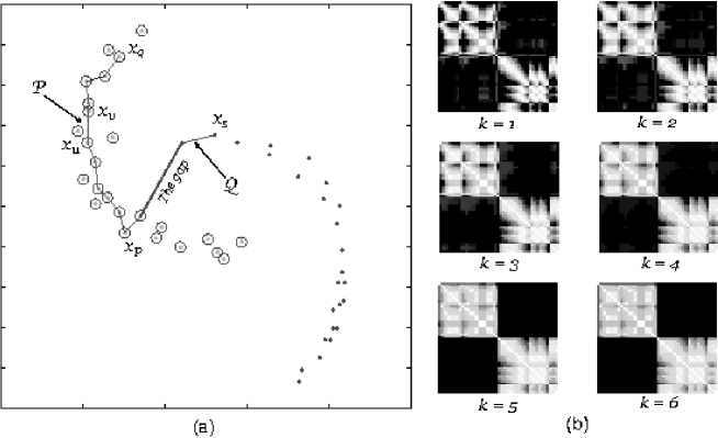
Figure 1: (a) A two-moon data set used to demonstrate the transitive distance, where samples of one cluster are denoted by circles and samples of another cluster are denoted by dots. (b) Maps of transitive distance matrices with different orders.

the distance between samples $x_{p}$ and $x_{q}$ is larger than that between $x_{p}$ and $x_{s}$ from the usual viewpoint of the Euclidean metric. A more reasonable metric on the data set should give a closer relationship (thus smaller distance) between $x_{p}$ and $x_{q}$ than that between $x_{p}$ and $x_{s}$ since $x_{p}$ and $x_{q}$ lie in the same cluster but $x_{p}$ and $x_{s}$ do not. A common method to overcome this difficulty is to create a non-linear mapping

$$\phi:V\subset R^{l}\rightarrow V^{\prime}\subset R^{s},$$ (1)

such that the images of any two clusters in $R^{s}$ can be split linearly. This method is called the kernel trick and is overwhelmingly used in recent clustering schemes. Usually the mapping that can reach this goal is hard to find. Besides, another problem arises when the size of the data set increases; these schemes usually depend on the solution to the eigenproblem, the time complexity of which is $O(n^{3})$ generally.

Can we have a method that can overcome the above two problems and still achieve the kernel effect? In Fig. 1(a), we observe that $x_{p}$ and $x_{q}$ are in the same cluster only because the other samples marked by a circle exist; otherwise it makes no sense to argue that $x_{p}$ and $x_{q}$ are closer than $x_{p}$ and $x_{s}$. In other words, the samples marked by a circle contribute the information to support this observation.

Let us also call each sample a messenger. Take $x_{u}$ as an example. It brings some messsage from $x_{p}$ to $x_{q}$ and vice versa. The way that $x_{p}$ and $x_{q}$ are closer than the Euclidean distance between them can be formulated as

$$D(x_{p},x_{q})\leq\max\{d(x_{p},x_{u}),d(x_{u},x_{q})\},$$ (2)

where $d(\cdot,\cdot)$ is the Euclidean distance between two samples, and $D(\cdot,\cdot)$ is the distance we are trying to find that can reflect the true relationship between samples. In (2), $x_{u}$ builds a bridge between $x_{p}$ and $x_{q}$ in this formulation. When more and more messengers come in, we can define a distance through $k$ of these messengers. Let $\mathcal{P}=x_{u_{1}}x_{u_{2}}\cdots x_{u_{k}}$ be a path with $k$ vertices, where $x_{u_{1}}=x_{p}$ and $x_{u_{k}}=x_{q}$. A distance between $x_{p}$ and $x_{q}$ with $\mathcal{P}$ is defined as

$$D_{\mathcal{P}}(x_{p},x_{q})=\max_{x_{u_{i}}x_{u_{i+1}}\in\mathcal{P}\atop 1\leq i\leq k-1}\{d(x_{u_{i}},x_{u_{i+1}})\}.$$ (3)

We show an example in Fig. 1(a), where a path $\mathcal{P}$ from $x_{p}$ to $x_{q}$ is given. The new distance between $x_{p}$ and $x_{q}$ through $\mathcal{P}$ equals $d(x_{u},x_{v})$, which is smaller than the original distance $d(x_{p},x_{q})$. For samples $x_{p}$ and $x_{s}$, there are also paths between them, such as the path $\mathcal{Q}$, which also result in new distances between them smaller than $d(x_{p},x_{s})$. However, no matter how the path is chosen, the new distance between $x_{p}$ and $x_{s}$ is always larger than or equal to the smallest gap between the two clusters as follows.

Given two samples in a data set, we can have many paths connecting them. Therefore we define the new distance, called the transitive distance, between two samples as follows.

Definition 1.

Given the Euclidean distance $d(\cdot,\cdot)$, the derived transitive distance between samples $x_{p},x_{q}\in V$ with order $k$ is defined as

$$D_{k}(x_{p},x_{q})=\min_{\mathcal{P}\in\mathbb{P}_{k}}\max_{e\in\mathcal{P}}\{d(e)\},$$ (4)

where $\mathbb{P}_{k}$ is the set of paths connecting $x_{p}$ and $x_{q}$, each such path is composed of at most $k$ vertices, $e\stackrel{{\scriptstyle def}}{{=}}x_{i}x_{j}$, and $d(e)\stackrel{{\scriptstyle def}}{{=}}d(x_{i},x_{j})$.

In Fig. 1(b), we show the maps of transitive distance matrices for the data set in Fig. 1(a) with orders from $1$ to $6$, where a larger intensity denotes a smaller transitive distance. In this data set, there are 50 samples, and the samples in each cluster are consecutively labeled. From these maps, we can see that when $k$ is larger, the ratios of the inter-cluster transitive distances to the intra-cluster transitive distances tend to be larger. In other words, if more messengers are involved, the obtained transitive distances better represent the relationship among the samples.

When the order $k=n$, where $n$ is the number of all the samples, we denote $D_{n}$ with $D$ for simplicity. The following proposition shows that $D$ is an ultrametric.

Proposition 1.

The transitive distance $D$ is an ultrametric on a given data set.

The proof of Proposition 1 is simple and omitted here. So given a data set $V$ and its distance matrix $E$, we can obtain another ultrametric distance matrix $E^{\prime}$ through Definition 1. In [6], an $O(n^{3})$ algorithm is given to derive $E^{\prime}$ from $E$. In Section 4, we propose an algorithm which is almost $O(n^{2})$ to obtain $E^{\prime}$.

It is worth mentioning that although we use $d(\cdot,\cdot)$ to denote the Euclidean distance for convenience in the previous discussion, we can replace $d(\cdot,\cdot)$ with any other traditional distance (metric) in Definition 1 and still have Proposition 1. Therefore, in what follows, $d(\cdot,\cdot)$ is used to denote any traditional distance.

2.2 Kernel Trick by the Transitive Distance

In this section, we show that the derived ultra-metric well reflects the relationship among data samples and a kernel mapping with a promising property can be obtained. First we introduce a lemma from [11] and [7].

Lemma 1.

Every finite ultrametric space consisting of $n$ distinct points can be isometrically embedded into a $n-1$ dimensional Euclidean space.

With Lemma 1, we have the mapping

$$\phi:(V\subset R^{l},D)\rightarrow(V^{\prime}\subset R^{s},d^{\prime}),$$ (5)

where $\phi(x_{i})=x^{\prime}_{i}\in V^{\prime}$, $s=n-1$, and $n$ is the number of points in a set $V$. We also have $d^{\prime}(\phi(x_{i}),\phi(x_{j}))=D(x_{i},x_{j})$, where $d^{\prime}(\cdot,\cdot)$ is the Euclidean distance in $R^{s}$, i.e., the Euclidean distance between two points in $V^{\prime}$ equals its corresponding ultrametric distance in $V$.

Before giving an important theorem, we define the consistency stated in Section 1 precisely.

Definition 2.

A labeling scheme $\{(x_{i},l_{i})\}$ of a data set $V=\{x_{i}|i=1,2,\cdots,n\}$, where $l_{i}$ is the cluster label of $x_{i}$, is called consistent with some distance $d(\cdot,\cdot)$ if the following condition holds: for any $y\notin C$ and any partition $C=C_{1}\cup C_{2}$, we have $d(C_{1},C_{2})<d(y,C)$, where $C\subset V$ is some cluster, $y\in V$, $d(C_{1},C_{2})\stackrel{{\scriptstyle def}}{{=}}\min_{{x_{i}\in C_{1}}\atop{x_{j}\in C_{2}}}d(x_{i},x_{j})$ is the distance between the two sets $C_{1}$ and $C_{2}$, and $d(y,C)\stackrel{{\scriptstyle def}}{{=}}\min_{x\in C}d(y,x)$ is the distance between a point $y$ and the set $C$.

The consistency requres that the intra-cluster distance is strictly smaller than the inter-cluster distance. This might be too strict in some practical applications, but it helps us reveal the following desirable property for clustering.

Theorem 1.

If a labeling scheme of a data set $V=\{x_{i}|i=1,2,\cdots,n\}$, is consistent with a distance $d(\cdot,\cdot)$, then given the derived transitive distance $D$ and the embedding $\phi:(V,D)\rightarrow(V^{\prime},d^{\prime})$, the convex hulls of the images of the clusters in $V^{\prime}$ do not intersect with each other.

The proof of the theorem can be found in Appendix A. An example of the theorem is illustrated in Fig. 2. A data set $V$ with $50$ points in $R^{2}$ is mapped (embedded) into $R^{49}$, a much higher dimensional Euclidean space, where the convex hulls of the two clusters do not intersect. Moreover, the Euclidean distance between any two samples in $V^{\prime}$ is equal to the transitive distance between these two samples in $V$. The convex hulls of the two clusters intersect in $R^{2}$ but do not in $R^{49}$, meaning that they are linearly separable in a higher dimensional Euclidean space. We can see that the embedding $\phi$ is a desirable kernel mapping.

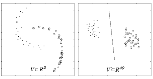
Figure 2: Mapping a set of 50 data samples in $V\subset R^{2}$ to $V^{\prime}\subset R^{49}$.

Obviously, the clustering of $V^{\prime}$ is much easier than the clustering of $V$. It seems that the K-means algorithm can be used to perform the clustering of $V^{\prime}$ easily. Unfortunately, we only have the distance matrix $E^{\prime}=[d^{\prime}_{ij}]=[D_{ij}]$ of $V^{\prime}$, instead of the coordinates of $x^{\prime}_{i}\in V^{\prime}$, which are necessary for the K-means algorithm. In Section 3, we explain how to circumvent this problem.

3 K-Means Duality

Let $E=[d_{ij}]$ be the distance matrix obtained from a data set $V=\{x_{i}|i=1,2,\cdots,n\}$. From $E$, we can derive a new set $Z=\{z_{i}|i=1,2,\cdots,n\}$, with $z_{i}\in R^{n}$ being the $i$th row of $E$. Then we have the following observation, called the duality of the K-means algorithm.

Observation (K-means duality): The clustering result obtained by the K-means algorithm on $Z$ is very similar to that obtained on $V$ if the clusters in $V$ are hyperellipsoid-shaped.

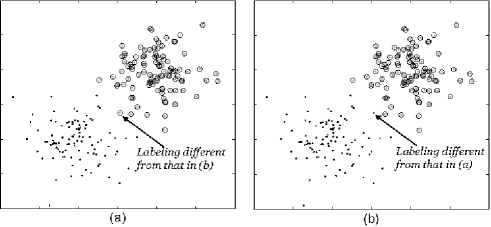
Figure 3: (a) Clustering result obtained by the K-means algorithm on the original data set $V$. (b) Clustering result obtained by the K-means algorithm on $Z$ derived from the distance matrix of $V$. Only one sample has different labelings from the two results.

We have this observation based on a large number of experiments on different data sets. Most data sets were randomly generated with multi-Gaussian distributions. From more than 100 data sets where each set contains 200 samples, we compared the results obtained by the K-means alogrithms on original data sets $V$’s and their corresponding sets $Z$’s. As a whole, the sample labeling difference is only 0.7%. One example is shown in Fig. 3, in which only one sample is labeled differently by the two clustering methods.

The matrix perturbation theory [16] can be used to explain this observation. We begin with an ideal case by supposing that the inter-cluster sample distances are much larger than the intra-cluster sample distances (obviously, the clustering on this kind of data sets is easy). In the ideal case, let the distance between any two samples in the same cluster be $0$. If the samples are arranged in such a way that those in the same cluster are indexed by successive integers, then the distance matrix will be such a matrix:

$$\hat{E}=\left(\begin{array}[]{cccc}E_{1}&\cdots&\cdots&\cdots\\ \cdots&E_{2}&\cdots&\cdots\\ \cdots&\cdots&\cdots&\cdots\\ \cdots&\cdots&\cdots&E_{k}\end{array}\right)\begin{array}[]{cl}\}&n_{1}~{}rows\\ \}&n_{2}~{}rows\\ {}\hfil&{}\\ \}&n_{k}~{}rows\end{array}$$ (6)

where $E_{i}=\mathbf{0},1\leq i\leq k$, represents the distance matrix within the $i$th cluster, $n_{1}+n_{2}+\cdots+n_{k}=n$, and $k$ denotes the number of clusters. Let $\hat{Z}=\{\hat{z}_{i}|i=1,2,\cdots,n\}$ with $\hat{z}_{i}$ being the $i$th row of $\hat{E}$. Then in this ideal case, we have $\hat{z}_{1}=\hat{z}_{2}=\cdots=\hat{z}_{n_{1}},\hat{z}_{n_{1}+1}=\hat{z}_{n_{1}+2}=\cdots=\hat{z}_{n_{1}+n_{2}},\cdots,\hat{z}_{n-n_{k}+1}=\hat{z}_{n-n_{k}+2}=\cdots=\hat{z}_{n}$. Therefore, if $\hat{Z}$ is considered as a data set to be clustered, the distance between any two samples in each cluster is still $0$. On the other hand, for two samples in different clusters, say, $\hat{z}_{1}$ and $\hat{z}_{n_{1}+1}$, we have

$$\hat{z}_{1} =(\overbrace{0,\cdots,0}^{n_{1}},d_{1,{n_{1}+1}},\cdots,d_{1,{n_{1}+n_{2}}},\cdots),$$ (7)

$$\hat{z}_{n_{1}+1} =(d_{n_{1}+1,1},\cdots,d_{n_{1}+1,n_{1}},\underbrace{0,\cdots,0}_{n_{2}},d_{n_{1}+1,n_{1}+n_{2}+1},\cdots),$$ (8)

and

$$d(\hat{z}_{1},\hat{z}_{n_{1}+1})\geq\sqrt{\sum_{j=n_{1}+1}^{n_{1}+n_{2}}d_{1,j}^{2}+\sum_{j=1}^{n_{1}}d_{n_{1}+1,j}^{2}}\gg 0.$$ (9)

Thus, the distance between any two samples in different clusters is still large. The distance relationship in the original data set is preserved completely in this new data set $\hat{Z}$. Obviously, the K-means algorithm on the original data set can give the same result as that on $\hat{Z}$ in this ideal case. In general cases, a perturbation $P$ is added to $\hat{E}$, i.e., $E=\hat{E}+P$, where all the diagonal elements of $P$ are zero. The matrix perturbation theory [16] indicates that the K-means clustering result on the data set $Z$ that is derived from $E$ is similar to that on $\hat{Z}$ if $P$ is not dominant over $\hat{E}$. Our experiments and the above analysis support the observation of the K-means duality.

Now we are able to give a solution to the problem mentioned at the end of Section 2.2. From Theorem 1, we can map a data set $V$ to $V^{\prime}\subset R^{n-1}$ where the clustering is easier if the clusters with the original distance are consistent in $V$. The problem we need to handle is that in $R^{n-1}$ we only have the distance matrix instead of the coordinates of the samples in $V^{\prime}$. From the analysis of the K-means duality in this section, we can perform the clustering based on the distance matrix by the K-means algorithm. Therefore, the main ingredients for a new clustering algorithm are already available.

4 A New Clustering Algorithm

Given a data set $V=\{x_{i}|i=1,2,\cdots,n\}$, our clustering algorithm is described as follows.

Algorithm 1 Clustering Based on the Transitive Distance and the K-means Duality

• Construct a weighted complete graph $G=(V,E)$ where $E=[d_{ij}]_{n\times n}$ is the distance matrix containing the weights of all the edges and $d_{ij}$ is the distance between samples $x_{i}$ and $x_{j}$.

• Compute the transitive distance matrix $E^{\prime}=[d^{\prime}_{ij}]=[D_{ij}]$ based on $G$ and Definition 1, where $D_{ij}$ is the transitive distance with order $n$ between samples $x_{i}$ and $x_{j}$.

• Perform clustering on the data set $Z^{\prime}=\{z^{\prime}_{i}|i=1,2,\cdots,n\}$ with $z^{\prime}_{i}$ being the $i$th row of $E^{\prime}$ by the K-means algorithm and then assign the cluster label of $z^{\prime}_{i}$ to $x_{i}$, $i=1,2,\cdots,n$.

In step 2), we need to compute the transitive distance with order $n$ between any two samples in $V$, or equivalently, to find the transitive edge, which is defined below.

Definition 3.

For a weighted complete graph $G=(V,E)$ and any two vertices $x_{p},x_{q}\in V$, the transitive edge for the pair $x_{p}$ and $x_{q}$ is an edge $e=x_{u}x_{v}$, such that $e$ lies on a path connecting $x_{p}$ and $x_{q}$ and $D_{pq}=D(x_{p},x_{q})=d(x_{u},x_{v})$.

An example of a transitive edge is shown in Fig. 1(a). Because the number of paths between two vertices (samples) is exponential in the number of the samples, the brutal searching for the transitive distance between two samples is infeasible. It is necessary to design a faster algorithm to carry out this task. The following Theorem 2 is for this purpose.

Without loss of generality, we assume that the weights of edges in $G$ are distinct. This can be achieved by slight perturbations of the positions of the data samples. After this modification, the clustering result of the data will not be changed if the perturbation are small enough.

Theorem 2.

Given a weighted complete graph $G=(V,E)$ with distinct weights, each transitive edge lies on the minimum spanning tree $\widetilde{G}=(V,\widetilde{E})$ of $G$.

The proof of Theorem 2 can be found in Appendix B. This theorem suggests an efficient algorithm to compute the transitive matrix $E^{\prime}=[d^{\prime}_{ij}]_{n\times n}$ which is shown in Algorithm 2. Next we analyze the computational complexity of this algorithm.

Algorithm 2 Computing the transitive distance matrix $E^{\prime}=[d^{\prime}_{ij}]_{n\times n}$

• Build the minimum spanning tree $\widetilde{G}=(V,\widetilde{E})$ from $G=(V,E)$.

• Initialize a forest $F\leftarrow\widetilde{G}$.

• Repeat

• For each tree $T\in F$ do

• • Cut the edge with the largest weight $w_{T}$ and partition $T$ into $T_{1}$ and $T_{2}$.

• For each pair $(x_{i},x_{j})$, $x_{i}\in T_{1}$, $x_{j}\in T_{2}$ do

• $d^{\prime}_{ij}\leftarrow w_{T}$

• End for

• End for

• Until each tree in $F$ has only one vertex.

Building the minimum spanning tree from a complete graph $G$ needs time very close to $O(n^{2})$ by the algorithm in [2]. When Algorithm 2 stops, total $n$ non-trivial tree have been generated. The number of the edges in each non-trivial tree is not larger than $n$. Therefore, the total time taken by searching for the edge with the largest weight on each tree (step 5) in the algorithm is bounded by $O(n^{2})$. Steps 6–8 are for finding the values for the elements of $E^{\prime}$. Since each element of $E^{\prime}$ is visited only once, the total time consumed by steps 6–8 is $O(n^{2})$. Thus the computational complexity of Algorithm 2 is about $O(n^{2})$.

Considering the time $O(n^{2})$ for building the distance matrix $E$, and the fact that the complexity of the K-means algorithm is close to $O(n^{2})$, we conclude that the computational complexity of Algorithm 1 is about $O(n^{2})$.

Although the minimum spanning tree is used to help clustering in both the hierarchical clustering and our algorithm, the motivations and effects are quite different. In our case, the minimum spanning tree is for generating a kernel effect (to obtain the relationship among the samples in a high dimensional space according to Theorem 1), with which the K-means algorithm provides a global optimization function for clustering. Whereas in the hierarchical clustering, each iteration step only focuses on the local sample distributions. This difference leads to distinct algorithms in handling the data obtained from the minimum spanning tree. We carry out the K-means algorithm on the derived $Z^{\prime}$ according to the K-means duality, while the hierarchical clustering cuts $c-1$ largest edges from the minimum spanning tree, where $c$ is the number of clusters. In Fig. 4, we show a data set clustered by the two approaches. The multi-scale data set makes the hierarchical clustering give an unreasonable result.

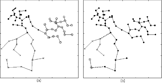
Figure 4: (a) The minimum spanning tree and the clustering result by our algorithm. (b) The minimum spanning tree and the clustering result by the hierarchical clustering. The dashed lines are the cutting edges. The number of clusters is 3.

5 Experiments

We have applied the proposed algorithm to a number of clustering problems to test its performance. The results are compared with those by the K-means algorithm, the NJW spectral clustering algorithm [13] and the self-tuning spectral clustering algorithm [18]. For each data set, the NJW algorithm needs manually tuning of the scale and the self-tuning algorithm needs to set the number of nearest neighbors. On the contrary, no parameters are required to set for our algorithm. In this comparisons, we show the best clustering results that are obtain by adjusting the parameters in the two spectral clustering algorithms. All the numbers of clusters are assumed to be known.

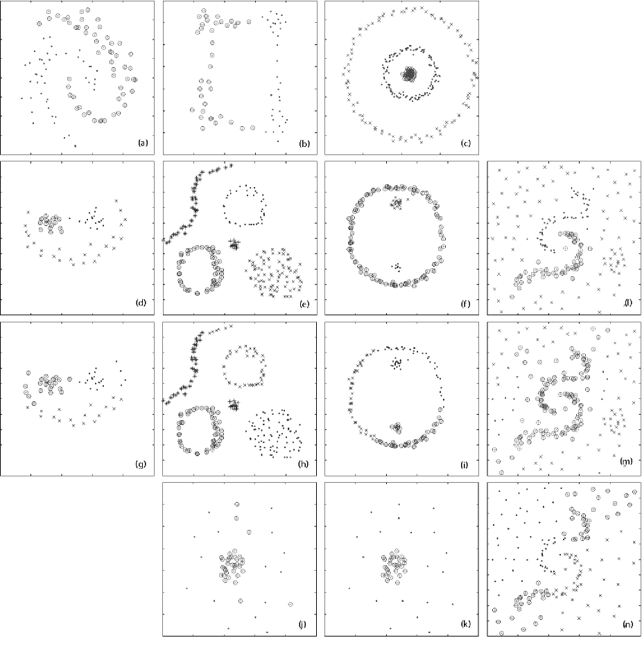
Figure 5: Clustering results by our algorithm and the two spectral algorithms. (a)(b)(c) Results by the three algorithms. (d)(e)(f) Results by the NJW algorithm and ours. (g)(h)(i) Results by the self-tuning algorithm. (j) Result by the NJW algorithm. (k) Result by the self-tuning algorithm and ours. (l)(m)(n) Results by our algorithm, the NJW algorithm, and the self-tuning algorithm, respectively.

5.1 Synthetic Data Sets

Eight synthetic data sets are used in the experiments. Bounded in a region $(0,1)\times(0,1)$, these data sets are with complex cluster shapes, multi-scale clusters, and noise. The clustering results are shown in Fig. 5. Note that the results obtained by the K-means algorithm are not given because it is obvious that it cannot deal with these data sets.

In Figs. 5(a)–(c), all the three algorithms obtain the same results. Figs. 5(d)–(f) and (g)–(i) show three data sets on which the self-tuning algorithm gives different results from the other two algorithms. The self-tuning algorithm fails to cluster the data sets no matter how we tune its parameter. Figs. 5(j) and (k) show two clustering results where the data set is with multi-scale clusters. The former is produced by the NJW algorithm and the latter by the self-tuning and our algorithms. To cluster the data set in Figs. 5(l)–(n) is a challenging task, where two relatively tightly connected clusters are surrounded by uniformly distributed noise samples (the third cluster). Our algorithm obtains the more reasonable result (Fig. 5(l)) than the results by another two algorithms (Figs. 5(m) and (n)).

From these samples, we can see that our algorithm performs similar to or better than the NJW and self-tuning spectral clustering algorithms. This statement applies to many other data sets we have tried, which are not shown here due to the limitation of space.

5.2 Data Sets from the USPS Database

USPS database is an image database provided by the US Postal Service. There are 9298 handwriting digit images of size $16\times 16$ from “0” to “9” in the database, from which we construct ten data sets from this database. Each set has 1000 images selected randomly with two, three, or four clusters. Each image is treated as a point in a 256-dimensional Euclidean space. The following figure shows the error rates of the four algorithms on these sets. In this experiments, the parameters for the NJW and self-tuning algorithms are tuned carefully to obtain the smallest error rates. These results show that as a whole, our algorithm achieves the smallest error rate, and the K-means and self-tuning algorithms perform worst.

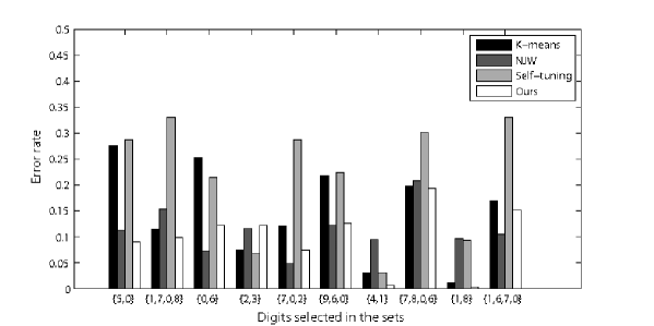
Figure 6: The error rates of the four algorithms on the ten data sets constructed from the USPS database.

5.3 Iris and Ionosphere Data Sets

We also test the algorithms on two commonly-used data sets, Iris and Ionosphere, in UCI machine learning database. Iris consists of 150 samples in 3 classes, each with 50 samples. Each sample has 4 features. Ionosphere contains 354 samples in 2 classes and each sample has 34 features. In Table 1 we show the error rates of the four algorithms clustering on these data sets. For the NJW and self-tuning algorithms, we have to adjust their parameters ($\delta$ and $N$) to obtain the smallest error rates, which are shown in the table. Our algorithm results in the smallest error rates among the four algorithms.

Table 1: Error rates of the four algorithms on Iris and Ionosphere data sets

	K-means	NJW	Self-tuning	Ours
Iris	0.11	0.09 ($\delta=0.40$)	0.15 ($N=5$)	0.07
Ionosphere	0.29	0.27 ($\delta=0.20$)	0.30 ($N=6$)	0.15

5.4 Remarks

From the experiments, we can see that compared with the K-means algorithm, our algorithm and the spectral algorithms can handle the clustering of a data set with complex cluster shapes. Compared with the spectral algorithms, our algorithm has comparable or better performance and does not need to adjust any parameter. In the above experiments, since we have the ground truth for each data set, we can try different parameters in the NJW and self-tuning algorithms so that they produce the best results. However, we do not know which parameters should be the best for unsupervised data clustering in many applications. Another advantage of our algorithm over the spectral algorithms is that its computational complexity is close to $O(n^{2})$, while the spectral algorithms’ complexities are $O(n^{3})$.

6 Conclusion

In this paper, we have built a connection between the transitive distance and the kernel technique for data clustering, By using the transitive distance, we show that if the consistency conditions is satisfied, the clusters of arbitrary shapes can be mapped to a new space where the clusters are easier to be seperated. Based on the observed K-means duality, we have developed an efficient algorithm with computational complexity $O(n^{2})$. Compared with the two popular spectral algorithms whose computational complexities are $O(n^{3})$, our algorithm is faster, without the need to tune any parameters, and performs very well. Our algorithm can be used to handle challenging clustering problems where the data sets are with complex shapes, multi-scale clusters, and noise.

7 Appendix A: Proof of Theorem 1

It is reasonable to assume that each cluster has at least two samples. Let $x_{i}$, $x_{j}\in C$, $x_{k}\notin C$, $x_{i}$, $x_{j}$, $x_{k}\in V$, where $C\subset V$ is some cluster. Then their images after the mapping $\phi$ are $x^{\prime}_{i}$, $x^{\prime}_{j}$, $x^{\prime}_{k}\in V^{\prime}$, where $x^{\prime}_{i}$, $x^{\prime}_{j}\in C^{\prime}$, $x^{\prime}_{k}\notin C^{\prime}$, and $C^{\prime}=\phi(C)$.

• First, we verify that if $d^{\prime}(x^{\prime}_{i},x^{\prime}_{j})\geqslant d_{0}\in R^{+}$, then there exists a partition $C_{1}\cup C_{2}=C$ such that $d(C_{1},C_{2})\geqslant d_{0}$. Such a partition can be obtained by the following steps:

  • Initialize $H=C$, $m=1$, $C_{1}=\emptyset$, and $C_{2}=\emptyset$.

  • Find a path $\mathcal{P}$ including the transitive edge from $x_{i}$ to $x_{j}$ in $H$.

  • Cut the transitive edge on the path $\mathcal{P}$. Let $\mathcal{P}_{m}$ ($\mathcal{Q}_{m}$) be the set consisting of the samples on $\mathcal{P}$ that are on the same side with $x_{i}$ ($x_{j}$) after the cutting, except $x_{i}$ ($x_{j}$).

  • $C_{1}\leftarrow C_{1}\cup\mathcal{P}_{m}$, $C_{2}\leftarrow C_{2}\cup\mathcal{Q}_{m}$, $H\leftarrow H\backslash\{\mathcal{P}_{m}\cup\mathcal{Q}_{m}\}$, and $m\leftarrow m+1$.

  • Repeat 2), 3), and 4) until only $x_{i}$ and $x_{j}$ are left in $H$.

  • $\mathcal{P}_{m}\leftarrow\{x_{i}\}$, $\mathcal{Q}_{m}\leftarrow\{x_{j}\}$, $C_{1}\leftarrow C_{1}\cup\mathcal{P}_{m}$, and $C_{2}\leftarrow C_{2}\cup\mathcal{Q}_{m}$.

  In this procedure, from (4) we can see that $d(\mathcal{P}_{s},\mathcal{Q}_{t})\geqslant d^{\prime}(x^{\prime}_{i},x^{\prime}_{j}),~{}1\leqslant s,t\leqslant m$. Since $C_{1}=\mathcal{P}_{1}\cup\mathcal{P}_{2}\cup\cdots\cup\mathcal{P}_{m}$ and $C_{2}=\mathcal{Q}_{1}\cup\mathcal{Q}_{2}\cup\cdots\cup\mathcal{Q}_{m}$, we have $d(C_{1},C_{2})=\min_{1\leqslant s,t\leqslant m}\{d(\mathcal{P}_{s},\mathcal{Q}_{t})\}$. Thus, $d(C_{1},C_{2})\geqslant d^{\prime}(x^{\prime}_{i},x^{\prime}_{j})\geqslant d_{0}$.

• Second, we show that there exist $x_{u}\in C$ and $x_{v}\notin C$ such that $d^{\prime}(x^{\prime}_{i},x^{\prime}_{k})\geqslant d(x_{u},x_{v})$. From Definition 1, we have a path $\mathcal{P}$ connecting $x_{i}$ and $x_{k}$ including the transitive edge. Then there exists an edge $x_{u}x_{v}\in\mathcal{P}$ such that $x_{u}\in C$ and $x_{v}\notin C$, and from (4), we have $d^{\prime}(x^{\prime}_{i},x^{\prime}_{k})\geqslant d(x_{u},x_{v})$.

• Third, we show that

  $$d^{\prime}(x^{\prime}_{i},x^{\prime}_{j})\leqslant\min\{d^{\prime}(x^{\prime}_{i},x^{\prime}_{k}),d^{\prime}(x^{\prime}_{j},x^{\prime}_{k})\}.$$ (10)

  Assume, to the contrary, that $d^{\prime}(x^{\prime}_{i},x^{\prime}_{j})>d^{\prime}(x^{\prime}_{i},x^{\prime}_{k})$. From (i) and (ii), we have a partition $C_{1}\cup C_{2}=C$, and $x_{u}\in C$, $x_{v}\notin C$ such that $d(C_{1},C_{2})\geqslant d^{\prime}(x^{\prime}_{i},x^{\prime}_{j})$ and $d^{\prime}(x^{\prime}_{i},x^{\prime}_{k})\geqslant d(x_{u},x_{v})$. Thus $d(C_{1},C_{2})\geqslant d^{\prime}(x^{\prime}_{i},x^{\prime}_{j})>d^{\prime}(x^{\prime}_{i},x^{\prime}_{k})\geqslant d(x_{u},x_{v})\geqslant d(C,x_{v})$, which contradicts the consistency of $V$. Therefore, (10) holds.

• Let $C=\{x_{c_{1}},\cdots,x_{c_{m}}\}$ be a cluster in $V$, with its image $C^{\prime}=\phi(C)=\{x^{\prime}_{c_{1}},\cdots,x^{\prime}_{c_{m}}\}\subset V^{\prime}$. Let $\widetilde{C}^{\prime}$ be the convex hull of $C^{\prime}$. Now we verify that no samples not in $C^{\prime}$ are in $\widetilde{C}^{\prime}$. Assume, to the contrary, that there exists a sample $y^{\prime}\in\widetilde{C}^{\prime}$, $y\notin C^{\prime}$. Consider a sample $x^{\prime}\in C^{\prime}$. Let $P$ be the hyperplane, each point on which has the same distance to $x^{\prime}$ and $z^{\prime}$. Then there must exist another sample $z^{\prime}\in C^{\prime}$ such that $y^{\prime}$ and $z^{\prime}$ are in the same side of $P$, which leads to $d^{\prime}(x^{\prime},z^{\prime})>d^{\prime}(y^{\prime},z^{\prime})$, a contradiction to (10).

In (iv), we have verified that for any cluster $C^{\prime}\in V^{\prime}$, no samples from other clusters can be in the convex hull of $C^{\prime}$. Thus, the convex hulls of all the clusters in $V^{\prime}$ are not intersecting each other.

8 Appendix B: Proof of Theorem 2

For any two distinct vertices $x_{1}$ and $x_{2}$ in $G$, let $\mathcal{P}=x_{k_{1}}x_{k_{2}}\cdots x_{k_{s}}$ be the path connecting them including the transitive edge $x_{k_{i}}x_{k_{i+1}}$, where $k_{1}=1$ and $k_{s}=2$. Then from Definition 1, we have

$$d(x_{k_{m}},x_{k_{m+1}})<d(x_{k_{i}},x_{k_{i+1}}),~{}m=1,2,\cdots,i-1,i+1,\cdots,s.$$ (11)

Next we verify that the edge $x_{k_{i}}x_{k_{i+1}}$ is in $\widetilde{G}$. Let $\widetilde{G}_{\mathcal{P}}=\widetilde{G}\cup\mathcal{P}$. Assume, to the contrary, that $x_{k_{i}}x_{k_{i+1}}\notin\widetilde{G}$. Then the edge $x_{k_{i}}x_{k_{i+1}}$ must be on a loop $\mathcal{O}\subseteq\widetilde{G}_{\mathcal{P}}$. Consider the following two cases:

• For any edge $x_{u}x_{v}\in\widetilde{G}\cap\mathcal{O}$, $d(x_{u},x_{v})<d(x_{k_{i}},x_{k_{i+1}})$.

• There exists an edge $x_{l_{j}}x_{l_{j+1}}\in\widetilde{G}\cap\mathcal{O}$ such that $d(x_{l_{j}},x_{l_{j+1}})>d(x_{k_{i}},x_{k_{i+1}})$.

Suppose that case (i) is true. Then for any edge on the path $(\mathcal{P}\cup\mathcal{O})\backslash\{x_{k_{i}}x_{k_{i+1}}\}$ that also connects $x_{1}$ and $x_{2}$, we have its length smaller than the transitive edge for $x_{1}$ and $x_{2}$. Thus case (i) cannot be true.

Suppose that case (ii) is true. Since $\widetilde{G}^{*}=(\widetilde{G}\cup\{x_{k_{i}}x_{k_{i+1}}\})\backslash\{x_{l_{j}}x_{l_{j+1}}\}$ is a spanning tree of $G$, and the sum of the edge weights in $\widetilde{G}^{*}$ is smaller than that in $\widetilde{G}$, we have a contradiction to the fact that $\widetilde{G}$ is the minimum spanning tree. Thus case (ii) cannot be true either, which completes the proof.

References

- [1] Y. Boykov and V. Kolmogorov. An experimental comparison of min-cut,max-flow algorithms for energy minimization in vision. IEEE Transactions on Pattern Analysis and Machine Intelligence, 26(9):1124–1137, 2004.
- [2] B. CHAZELLE. A minimum spanning tree algorithm with inverse-Ackermann type complexity. Journal of the ACM, 47(6):1028–1047, 2000.
- [3] D. Comaniciu and P. Meer. Mean shift: a robust approach toward feature space analysis. IEEE Transactions on Pattern Analysis and Machine Intelligence, 24(5):603–619, 2002.
- [4] JW de Bakker and JI Zucker. Denotational semantics of concurrency. Proceedings of the 14th Annual ACM Symposium on Theory of Computing, pages 153–158, 1982.
- [5] I.S. Dhillon, Y. Guan, and B. Kulis. Kernel k-means: spectral clustering and normalized cuts. Proceedings of the 2004 ACM SIGKDD International Conference on Knowledge Discovery and Data Mining, pages 551–556, 2004.
- [6] C. Ding, X. He, H. Xiong, and H. Peng. Transitive closure and metric inequality of weighted graphs: detecting protein interaction modules using cliques. International Journal of Data Mining and Bioinformatics, 1(2):162–177, 2006.
- [7] M. Fiedler. Ultrametric sets in euclidean point spaces. Electronic Journal of Linear Algebra, 3:23–30, 1998.
- [8] M. Girolami. Mercer kernel-based clustering in feature space. IEEE Transactions on Neural Networks, 13(3):780–784, 2002.
- [9] A. K. Jain, M. N. Murty, and P. J. Flynn. Data clustering: a review. ACM Computing Surveys, 31(3):264–323, 1999.
- [10] S.C. Johnson. Hierarchical clustering schemes. Psychometrika, 32(3):241–254, 1967.
- [11] A.Y. Lemin. Isometric imbedding of isosceles (non-Archimedean) spaces into Euclidean ones. Dokl. Akad. Nauk SSSR, 285:558–562, 1985.
- [12] J. MacQueen. Some methods for classification and analysis of multivariate observations. Proceedings of 5th Berkeley Symposium on Mathematical Statistics and Probability, Berkeley, 1:281–297, 1967.
- [13] A.Y. Ng, M. Jordan, and Y. Weiss. On spectral clustering: Analysis and an algorithm. Advances in Neural Information Processing Systems, 14(2):849–856, 2001.
- [14] R.D.M. Page, E. Holmes, and D.E.C. Holmes. Molecular Evolution: A Phylogenetic Approach. Blackwell Publishing, 1998.
- [15] J. Shi and J. Malik. Normalized cuts and image segmentation. IEEE Transactions on Pattern Analysis and Machine Intelligence, 22(8):888–905, 2000.
- [16] G.W. Stewart and J. Sun. Matrix Perturbation Theory, Computer Science and Scientific Computing, 1990.
- [17] D. Verma and M. Meila. A comparison of spectral clustering algorithms. Technical report 03-05-01, Department of Computer Science and Engineering, University of Washington, 2003.
- [18] L. Zelnik-Manor and P. Perona. Self-tuning spectral clustering. Advances in Neural Information Processing Systems, 17:1601–1608, 2004.