The WFCAM Science Archive

Abstract

We describe the WFCAM Science Archive (WSA), which is the primary point of access for users of data from the wide–field infrared camera WFCAM on the United Kingdom Infrared Telescope (UKIRT), especially science catalogue products from the UKIRT Infrared Deep Sky Survey (UKIDSS). We describe the database design with emphasis on those aspects of the system that enable users to fully exploit the survey datasets in a variety of different ways. We give details of the database–driven curation applications that take data from the standard nightly pipeline–processed and calibrated files for the production of science–ready survey datasets. We describe the fundamentals of querying relational databases with a set of astronomy usage examples, and illustrate the results.

1 Introduction

The term ‘science archive’ is first seen in the astronomy literature in Barrett (1993) which describes the High Energy Astrophysics Science Archive Research Centre (HEASARC). This system is much more than a simple repository of data – HEASARC provides an online resource to enable scientific exploitation of high–energy astronomy missions via provision of science data, software, analysis tools and descriptive information. For example, the data holdings in the HEASARC amount to many terabytes (TB; 1 TB=10¹² bytes) so wholesale download is impractical; recognising this, a server–side analysis facility (i.e. a facility co-located with the data and hence remote to the typical user) is provided to enable large–scale processing given an arbitrary astronomical usage scenario. In this way, data download is limited to user–defined subsets, sometimes processed in a manner specified by the user at access time.

The advent of the large Schmidt photographic plate digitisation programmes (Hambly et al. 2001a and references therein) and infrared surveys such as DENIS (Epchtein et al. 1994) and 2MASS (Kleinmann et al. 1994) presented similar challenges for ground–based missions. Data distribution for the digitised Schmidt surveys was originally done on removable, permanent storage media (‘compact disc’ read–only memory), but this became impractical so online services rapidly developed for these also. However, it is probably fair to say that it was with the challenges posed by the Sloan Digital Sky Survey (SDSS; York et al. 2000) that the ground–based astronomical science archive became fully developed (Gray et al. 2002). The first SDSS (the so–called Sloan Legacy Survey) is now complete, and $\sim 2\times 10^{8}$ sources have been measured and characterised, producing a catalogue of several TB in size with associated imaging data and $\sim 10^{6}$ spectra amounting to a total volume of $\sim 10$ TB (Adelman–McCarthy et al. 2007 and references therein); the state–of–the–art SDSS science archive is described in Thakar et al. (2003a).

The challenges and opportunities presented by the current generation of ground–based infrared surveys were noted by Lawrence et al. (2002). In particular, they cited the advent of a new wide–field camera for the 4-m United Kingdom Infrared Telescope (WFCAM for UKIRT; Casali et al. 2007) and the even greater challenges posed by the new dedicated 4-m telescope for infrared surveys VISTA (Emerson 2001). These ambitious survey missions gave rise to a systems–engineered data management project, the VISTA Data Flow System (VDFS; Emerson et al. 2004) which included provision of pipeline processing and science archiving for WFCAM and VISTA data. Here, we concentrate on the first VDFS science archive known as the WFCAM Science Archive (WSA). From the outset, the design of the WSA has been science–driven with the main science stake–holders being users of the UKIRT Infrared Deep Sky Survey (UKIDSS; e.g. Warren 2002).

This paper is one of a set of five which provide the reference technical documentation for UKIDSS, although it is of direct relevance to any user of the WFCAM Science Archive. The other four papers in the series describe the infrared survey instrument itself (WFCAM; Casali et al. 2007); the WFCAM photometric system (Hewett et al. 2006); the UKIDSS surveys (Lawrence et al. 2007); and the pipeline processing system (Irwin et al. 2007).

This paper is arranged as follows. In Section 2, we describe the design of the WSA, concentrating on the development of the science requirements into data models (i.e. the database design) as presented to the end–user at access time. In Section 3 we discuss various detailed implementation issues that in particular inform the user as to how science–ready survey catalogues are generated from the standard flat file products processed by the nightly pipeline. Section 4 then goes on to discuss some illustrative science examples by concentrating on the expression of certain specific science usage modes in Structured Query Language (SQL), the lingua franca of relational database users. Following the usual conclusion, acknowledgements and bibliography we present as appendices some supplementary information to aid first–time users of the WSA.

2 Design

In this paper, we concentrate on those aspects of the design that are relevant to the end user, assumed to be an astronomer interested in exploiting the archive for the purposes of scientific research. Further background information, and in particular technical details of the Information Technology aspects of the overall VISTA Data Flow System can be obtained from a set of papers appearing in recent volumes of the Astronomical Data Analysis and Software Systems (ADASS) and the International Society for Optical Engineering (SPIE) publications series – see Hambly et al. (2004a), Collins et al. (2006), Emerson et al. (2006) and Cross et al. (2007). The design of the WSA is based, in part, on that of the science archive system for the SDSS (Thakar et al. 2003a and references therein). In particular, we have made extensive use of the relational design philosophy of the SDSS science archive, and have implemented some of the associated software modules (e.g. that for the computation and use of Hierarchical Triangular Mesh indexing of spherical coordinates – see Kunszt et al. 2000). Scalability of the design to terabyte data volumes was prototyped using our own existing legacy Schmidt survey dataset, the SuperCOSMOS Sky Survey (Hambly et al. 2001a and references therein). The resulting prototype science archive system, the SuperCOSMOS Science Archive (SSA) is described in Hambly et al. (2004b) and provides an illustration of the contrast in end–user experience of an old–style survey interface (as described in Hambly et al. 2001) and the new. Note that extensive technical design documentation for the WSA is maintained online.

The following Sections provide more information on the design to a level of detail that will enable a general user of the WSA to understand and to get the highest possible return out of the system.

2.1 Background

The WSA is a system designed to store, curate and serve all observations made by WFCAM, which is described in detail in Casali et al. (2007). The infrared active part of the focal plane consists of four $2048\times 2048$ detectors with plate scale 0.4″ pix^-1 arranged in a square pattern and spaced by 94% of the detector width (e.g. Casali et al. 2007, Figure 2). Hence, a sequence of four pointings is required to produce contiguous areal coverage of 0.78 sq. deg. (this is sometimes called a tile); however the unit of WSA curation (e.g. frame association for source merging – see later) is based around images of the size of one detector (known as a detector frame). Such an image is usually the result of stacking of a set of dithered and/or microstepped individual exposures (known as normal frames in the VDFS). Dithering (also known as jittering) is typically executed in step patterns of several arcseconds about a base position to allow for the removal of poor quality pixels at the processing stage. Microstepping, on the other hand, is sometimes used to recover full PSF sampling as the image quality delivered by WFCAM/UKIRT often can be better than the Nyquist limit of $\sim 0.8$″ given the 0.4″ WFCAM pixels. WFCAM instrument performance is concisely summarised in Casali et al. (2007), Table 3: e.g. median (best) image quality is 0.7″ (0.55″) at zenith at K band.

Observing time with WFCAM on UKIRT is divided between large scale surveys (i.e. UKIDSS and the recently instigated ‘campaigns’), smaller PI–led projects (awarded time via a telescope time allocation group), ‘service’ mode observations for very small projects requiring only a few hours of time, and special projects like observatory/survey infrastructure (calibration) and director’s discretionary time projects. Data from all these is tracked in the WSA, but the design is dictated primarily by the largest surveys, i.e. UKIDSS, which is described in detail in Lawrence et al. (2007).

Briefly, UKIDSS consists of a hierarchy of five surveys that trade depth versus area to cover a multitude of science goals. The Large Area Survey (LAS) aims to cover $\sim 4000$ sq. deg. in four infrared passbands to depths Y $\sim 20.3$, J $\sim 19.8$, H $\sim 18.6$ and K $\sim 18.2$ with two epochs of coverage at J. The Galactic Plane Survey (GPS) aims to cover $\sim 1900$ sq. deg. to depths J $\sim 19.9$, H $\sim 19.0$ and K $\sim 19.0$ with two (originally three) epochs of coverage at K and some coverage at narrow–band H2. The Galactic Clusters Survey (GCS) will survey ten open–cluster/star–formation regions to a total of $\sim 1000$ sq. deg. to depths Z $\sim 20.4$, Y $\sim 20.3$, J $\sim 19.5$, H $\sim 18.6$ and K $\sim 18.6$ with two epochs of coverage at K. The Deep eXtragalactic Survey (DXS) aims to survey four selected areas to a total of $\sim 35$ sq. deg. to depths J $\sim 22.3$, H $\sim 21.8$ and K $\sim 20.8$. Finally, the Ultra Deep Survey (UDS) aims to survey $\sim 0.8$ sq. deg. to depths J $\sim 24.8$, H $\sim 23.8$ and K $\sim 22.8$. UKIDSS LAS (J), GPS (JHK), GCS (K) and DXS (JK) employ $2\times 2$ microstepping (yielding 0.2″ samples) while the UDS employs $3\times 3$ microstepping in all filters (yielding 0.13″ samples). In the VDFS, an image resulting from interleaving microstepped frames is known as a leav frame while an image resulting from stacking a set of dithered exposures is known as a stack. An interleaved, stacked image is known as a leavstack frame – for many more details of VDFS pipeline processing, see Irwin et al. (2007). Survey data quality obtained in practice is summarised in UKIDSS data release papers (e.g. Dye et al. 2006; Warren et al. 2007a). Median seeing at Data Release 1 was $\sim 0.83$″; uniformity of photometric calibration as estimated via field–to–field scatter was between 0.02 and 0.03 mag in Y–J, J–H and H–K; mean stellar ellipticity was $\sim 0.08$. Observing strategies for UKIDSS are discussed extensively in Lawrence et al. (2007). Tiling the wide, shallow surveys, especially at high Galactic latitude, is dictated largely by the availability of suitable guide stars (V $<17$; Casali et al. 2007). This results in varying degrees of frame overlap and non–uniform tiling. The WSA copes with this via a data–driven source merging philosophy, and a flexible seaming algorithm for the production of interim catalogue products during the 7 year UKIDSS observing campaign, as is required to maximise timely scientific exploitation. Furthermore, a requirement exists for associating multiple–epoch visits of the same field, in addition to merely associating different passband visits. Again, a database–driven application ensures that sensible frame associations are made in the presence of incomplete datasets when intermediate releases are required before full survey completion.

In WSA parlance, UKIDSS as a whole is referred to as a survey while the LAS, GPS, DXS etc. are known as programmes (the rest, including PI–led programmes, are known as non–survey programmes). For the purposes of book–keeping at the observatory, observing is broken up into chunks known as projects which have a unique name that may include a Semester identification (e.g. u/07a/32 for non–survey PI–led programme no. 32 in Semester 07A; u/ukidss/gcs5 for UKIDSS GCS project observing set no. 5). The various survey and non–survey processed datasets stored and served in the WSA have proprietary periods ranging from 12 months for non–survey programmes to 18 months for the larger campaigns and surveys. These periods run from the time at which the processed data are made available to the respective proprietors rather than individual frame observing dates. Note that UKIDSS is proprietary to astronomers in the European Southern Observatory member states, while campaign and non–survey datasets are proprietary to the respective PIs and their named collaborators.

2.2 Archive requirements

A set of top–level general requirements was established early in the history of the WSA project. Briefly, requirements were specified in the following broad categories: i) top–level; ii) general contents and functions; iii) detailed functional requirements; and iv) security. Examples include i) broad–brush requirements concerning flexibility, scalability, ease–of–use and scope, e.g. the WSA is required to hold all pipeline–processed WFCAM data, not just that belonging to survey programmes (UKIDSS); ii) minimal requirements concerning contents and functionality, e.g. contents to include pixel, catalogue and associated metadata, along with calibration data; iii) a set of detailed functional requirements from the point of view of the end–user, e.g. searching and visualisation functionality required in the user interface; and finally iv) security rules concerning protection of the data itself, its integrity and any proprietary rights thereof.

In order to progress the design of the WSA from the top–level generalities summarised above, we followed a rational process similar to that employed in the design of the science archive for the SDSS (Thakar et al. 2003a), viz. the development of a set of questions and usage modes that one would ask or require of the archive to fulfill the functional requirements previously identified. This may seem somewhat ad hoc compared with a standard, ‘unified rational process’ (such as is encapsulated in Unified Modelling Language design, e.g. Gaessler et al. 2004 and references therein) but it has been successfully employed in the past (not least in the SDSS science archive design) and is rather powerful, despite its relative simplicity. We developed a set of 20 curation usage modes for the WSA and a set of 20 end–user usage modes in collaboration with the UKIDSS user community (see Appendix A). These were then analysed along with the original top–level requirements to produce a requirements analysis document to inform the detailed design described below. The design documents are all available online.

2.3 Design fundamentals

The WSA receives processed data from the pipeline component of the overall data flow system in the form of FITS (Hanisch et al. 2001) image and catalogue binary table files (Irwin et al. 2007). No raw pixel data are held in the WSA. Processed data consists of instrumentally–corrected WFCAM frames, associated descriptive and calibration data (including confidence frames and calibration images, e.g. darks and flats) and single–passband detection lists derived from the science frames. Calibration information also includes astrometric and photometric coefficients derived using the 2MASS (Skrutskie et al. 2006) point source catalogue as a reference. Metadata, meaning in this context those data that describe the imaging observations and processing thereof (e.g. observing dates/times, filters, instrument state, weather conditions, processing steps, etc.), are defined by a set of descriptor keywords agreed between the archive and pipeline centres, and include all information propagated from the instrument and observatory, along with additional keywords that describe the processing applied to each image and catalogue in the pipeline. Single passband detection catalogues for each science image have a standard set of 80 photometric, astrometric and morphological attributes along with error estimates, and a variety of summary quality control measures (e.g. seeing, average point source ellipticity etc.). For many more details, see Irwin et al. (2007).

The design of the WSA was based, from the outset, on a classical client–server architecture employing a third–party back–end commercial database management system (DBMS). This followed similar but earlier developments for the SDSS science archive, and reflects the great flexibility of such a system from the point of view of both applications development and end–user querying. Furthermore, although originally built (Szalay et al. 2000) on an ‘object oriented’ database, issues with performance and ease of use by the end user led to a switch to a relational database management system (RDBMS; a system that presents data as a group of related tabular data sets) in that project (Thakar et al. 2003b) and the WSA has been based on the relational model from the start. This brings many advantages for astronomy applications (indeed, for applications in any scientific discipline) where related sets of tabular information are familiar. Such advantages will be illustrated below; at this point we emphasise a few fundamental aspects of the relational design.

2.3.1 Default values and ‘not null’

As always in database design, a decision has to be made as to how to deal with the situation when no measurement is available to populate a particular field of a given row. For example, it may be that the data model (see later) requires that a merged source table has columns for infrared colours (J–H). What happens when H, or J, or even both are unavailable for that particular source (perhaps the images in these filters have not been taken yet, but we require to allow users access to the data that do exist for this source – e.g. observations in other filters)? This particular attribute, (J–H), could be set to a specified default value (an appropriately out–of–range but nonetheless real number, say $-0.999999\times 10^{9}$) or it can be allowed to be undefined (‘null’) in the RDBMS. One of the (many) problems with null values is that they complicate querying of the database: it is easier and clearer to ask “give me all the objects with (J–H) in the range 0.5 to 1.0” than it is to ask the same question with the additional predicate “and (J–H) is not null” (necessary because the RDBMS returns null values in results sets as a standard data type to be handled by querying applications). By judicious choice of default values, we can force exclusion of those rows where no measurement is available in an explicit and clear manner (in this case because the default value is outwith the range of a typical colour selection) thus simplifying querying applications. In this simple example this may seem rather unimportant but in more complicated situations the use of default values can greatly simplify querying applications and, as we describe later, the WSA philosophy is to expose the full power of the RDBMS to the end user for complete flexibility in querying. The WSA employs the default values as specified in Table 1 for the various data types listed, and does not allow null attributes in any column of any table.

2.3.2 Physical units

Physical quantities in the WSA are stored in SI units wherever possible. Astronomical convention dictates the usual standards for many astrophysical quantities; a conventional magnitude scale on the natural WFCAM system (Hewett et al. 2006) is employed for calibrated fluxes. All timestamps employed in the data flow system, including the science archive, are ‘Universal Time Coordinate’ (UTC) date/times. Spherical coordinates are stored in equatorial (J2000.0 equinox), Galactic and SDSS $(\lambda,\eta)$ coordinates (Stoughton et al. 2002) for ease of querying in different systems, and all angles (RA, Dec etc.) are stored in units of decimal degrees apart from a small number of image attributes that map directly to FITS keywords delivered by the pipeline. Equatorial coordinates at equinox J2000.0 are labelled with a 20–level Hierarchical Triangular Mesh index (Kunszt et al. 2000) to make spatially limited queries efficient.

2.3.3 Miscellaneous fundamentals

Pixel data are stored as flat files in the WSA system, rather than as ‘binary large objects’ in DBMS tables. This is so that high data volume usages (i.e. those requiring access to pixel data) that are not time–critical will not impact catalogue querying, where more ‘real–time’ performance is required for data exploration and interaction. However, pixel file names and the pixel metadata are tracked in tables within the DBMS so that the image descriptors can be browsed and queried in the same way as, or in conjunction with, catalogue data.

The WSA is organised as a self–describing database. This means that curation information, i.e. information pertaining to database–driven activities (for both invocation and results logging) in preparation of science–ready data products (see later) is contained in the database, along with science data. For example, the requirements for source merging for a survey programme (the filter selection and the number of passes in each filter, the source pairing criterion, etc.) are stored in database tables to drive the relevant curation activity and to inform users of the procedure.

Table 1: Default values for various data types in the WSA database.

Default value	Data type
$-0.9999995\times 10^{9}$	Floating point (single/double precision)
$-99999999$	Integer (4– and 8–byte)
$-9999$	Integer (2–byte)
NONE	Character
9999–Dec–31	Date–times

2.4 The WSA relational model

A good design for a relational database captures the structure inherent in the data to be stored, thereby aiding curation operations and end–user query modes, as these are both likely to reflect that structure. In conventional relational design, this structure is captured in an entity–relational model (ERM), in which a collection of related data is represented by an entity and entities have relationships between them, which can be mandatory or optional and can have one of three cardinalities (one–to–one, one–to–many or many–to–many).

To illustrate this, consider a processed WFCAM image file, as delivered by the pipeline (Irwin et al. 2007). Such a multi–extension FITS (MEF) file consisting of a primary header–data unit with generic descriptive keywords (observation date/time, filename, telescope/instrument parameters etc.) and a set of extensions containing the images and corresponding descriptive data of individual detectors can be represented in relational terms as in Figure 1. Here, we identify entities Multiframe and MultiframeDetector and a one–to–many relationship between them, each entity containing attributes that describe it. A particularly important point to note here is that the arrangement of data as represented in Figure 1 is normalised in the sense that we do not duplicate attributes in entity MultiframeDetector that pertain to a set of individual extension frames in each Multiframe – e.g. we could represent the data using a single entity where each set of detector frames (four in the case of WFCAM MEF file of a typical observation) is described by the generic attributes in entity Multiframe in addition to the specific attributes pertaining to each. Clearly, in terms of storage it is more efficient to have one record of the generic attributes of each set of detector frames, and link each MultiframeDetector to its parent Multiframe using a label and a reference in the RDBMS. Note that there is no requirement here for every Multiframe to have exactly four detector frames. A mosaiced image product can be equally well described by this data model – there will simply be a single extension representing the whole image, and the mosaic Multiframe will simply have one related row in MultiframeDetector.

In designing the WSA relational model, normalisation has been used except in a small number of cases where it makes sense to denormalise and duplicate some attributes for ease of use and better performance at query time; this is illustrated later, along with example usage modes requiring to query a set of normalised tables (‘join’ queries). The principle of normalisation complicates the data model for the novice user, but it is extremely important when designing a system that must scale to very large data volumes.

Experience with the SDSS has shown that scientifically realistic queries often require inclusion of constraints on metadata parameters and selection of rows on the basis of their provenance (e.g. properties of their parent images). To do this requires the user to know the basic structure of the database, so, in the remainder of this Section we describe the principal contents of the WSA in terms of ERMs, at a level which will enable users to define the queries they need to run to do their science.

Figure 1: A simple ‘entity–relationship’ model (ERM) showing in schematic form the relationship between the generic attributes of a multi–extension FITS image (a Multiframe in WSA parlance) and the particular attributes of each constituent image (MultiframeDetector) of that multiple image container file. The one–to–many (in fact one–to–four in the case of WFCAM) relationship between these two entities is represented by the ‘crows foot’ connecting the boxes (see text for a more detailed explanation).

2.4.1 Image data

As noted previously, image metadata are tracked in the WSA database, although the image pixel data themselves are not ingested into the RDBMS – they are stored as flat files on disk. In Figure 2 we show the ERM for pixel data in the WSA. Each entity box represents a database table, and one–to–many relationships between the tables are shown, as before. Note that some relationships are mandatory whereas some are optional. An example of a mandatory relationship is that every Multiframe has one or more MultiframeDetectors (not unreasonably, since a MEF devoid of any detector frames is not particularly useful). An example of an optional relationship, denoted by a dashed line on the side where the relationship is optional, is that every Filter might have one or more Multiframes (again, not unreasonable since there may be unused filters present in WFCAM) and yet every Multiframe has to have one associated filter record only. In this case, the mandatory relationship implies that there must always be a link between the Multiframe and Filter tables, even if that link points to a blank filter record, or if the filter keyword in a given Multiframe was unavailable for some reason, then the link will take a default value (see previously). However, to maintain referential integrity in the database there will need to be a default row in table Filter that can be referenced by the default link. This situation can occur in any part of the WSA data model where a mandatory relationship exists between two tables.

Figure 2: Relational model for image data in the WSA. Each box represents a table in the database; the lists of attributes in each are for illustration only, and are not intended to be complete. The ‘crows feet’ illustrate one–to–many relationships between data entries in each entity; dotted lines indicate optional as opposed to mandatory relationships (see text for further details).

Another useful feature of these ERM schematics is the indication of a unique identifier using the ‘#’ sign in the attribute list (a convention in entity–relationship modelling). Unique identifiers (UIDs) are, of course, key to efficient operation in a DBMS – without them, a table is simply a heap of data in which a specific row cannot be found easily. With a UID, on the other hand, every row of a table is uniquely labelled and can be located quickly, especially if the table data are sorted on that attribute (as is generally the case). Note that barred relationships in Figure 2 indicate where the combination of UIDs in both tables linked by the relationship are used, in the table on the barred side, as a combined UID. In the case of Multiframe and MultiframeDetector, for example, the UID in the former is simply a running number assigned on ingest, while in the latter the UID is a combination of the parent Multiframe UID plus the extension number – in this way, every MultiframeDetector is uniquely identified (it is conventional in ERMs to omit as ‘#’ UID attributes those UIDs from a related table, but we have explicitly noted them for clarity).

Other types of relationship are shown in Figure 2, and they illustrate how the WSA tracks the processing history, or provenance, of each processed image. Entity Provenance tracks the ancestor images of any image in the WSA that is the result of a combinatorial process on other images also tracked in the archive; hence for a Multiframe composed of $N$ other Multiframes (e.g. a stack of individual dithered Multiframes) this would contain $N$ records, each consisting of the UID of the final stack product (the attribute labelled as combiframeID) along with one of each of the $N$ separate constituent Multiframe UIDs; the other optional one–to–many relationship between entities Provenance and Multiframe indicates that every component frame recorded in the former must be present in the latter, while every Multiframe may be included as a constituent frame in one or more combined frame products. Finally, there is an optional self–referencing relationship indicated in the lower right–hand corner of entity Multiframe. This indicates that each Multiframe may be a pixel value correction frame used in the processing of one or more science Multiframes (there is an attribute to distinguish between different Multiframe types); conversely, each Multiframe may have been processed using one or more of each of the correction frame types dark, flat, sky etc. The relationship is optional on both sides since, for example, a flat will not itself be calibrated against a flat; moreover every single calibration frame that is propagated through the system may not get used in the processing of any science frames.

2.4.2 General catalogue data model

In Figure 3 we show a generalised ERM for catalogue data in the WSA. A set of five entities are identified that link with each other and with entity MultiframeDetector (see Figure 2) as shown. Briefly, standard 80–parameter detection lists from science images delivered by the pipeline (Irwin et al. 2007) are tracked in entity Detection; hence every MultiframeDetector may give rise to one or more Detections with a UID that includes the UID of the former. End–user science requirements, however, specify that most science applications need a merged, multi–colour, multi–epoch source list for convenience, so this data model includes an entity Source to track merged source records produced by a standard curation procedure (see later). Each Source is always made up of one or more individual passband Detections. The source merging procedure operates on sets of MultiframeDetectors where a frame set comprises detector frames taken at the same position but in different filters and/or at different times. These frame sets are tracked by entity MergeLog where every MergeLog frame set always consists of one or more MultiframeDetectors while an individual frame in the latter may or may not be a member of a frame set – non–science frames would not be included in frame sets, for example. The final two entities in Figure 3 are included to track enhanced catalogue extraction data from a process known colloquially as list–driven remeasurement. Standard pipeline processing treats each science image separately and extracts sources using a set of standard apertures and adaptive profile models applied at positions having detections above a sky noise–dependent threshold as described in Irwin et al. (2007). In the list–driven remeasurement scenario, a frame set is reanalysed for photometric attributes amongst all individual frames in the set using a master list of sources that are present in the field and a single set of apertures and models to yield photometric attributes consistently measured across the frame set. In this way, attributes such as colours are measured in a usefully consistent way, e.g. at the same position and with the same profile model, across all available passbands. In many ways, entities ListRemeasurement and SourceRemeasurement are analogous to Detection and Source respectively and hence show similar relationships between each other and MultiframeDetector. However, every SourceRemeasurement is driven by one Source – this defines the one–to–one relationship between these entities. Futhermore, certain photometric attributes of the remeasurement entities will have slightly different meanings to their analogues in Detection and Source, most notably flux measurements at positions defined by the driving list. In order to cope with the possibility of marginally detected or negative fluxes, one approach (which has yet to gain wide acceptance in the astronomical literature) is to adopt the magnitude scale of Lupton, Gunn & Szalay (1999) in the remeasurement entities for any calibrated flux attributes to be usefully defined in such a situation. (We note that at the time of writing, list–driven photometry has yet to be implemented in the WSA).

Figure 3: Generalised relational model for catalogue data in the WSA (see text).

It is important to note that the WSA is required to track a number of different science programmes in which the prescription for source merging (i.e. the required filters and number of distinct epoch passes in those filters) will be different. Before illustrating a specific example of the application of the generalised catalogue ERM, we need to discuss the top–level data model of the WSA that describes the observational programmes contained within it.

2.4.3 Top–level metadata

In order to track the various programmes for which the WSA is required to hold data, e.g. survey (UKIDSS), non–survey (private proprietary) and ‘service’ programmes, the set of entities in the schematics in Figures 4 and 5 have been identified. Consider the UKIDSS survey, which consists of five sub–survey components. Once again, in simple relational terms we identify entity Survey with a mandatory one–to–many relationship to a set of Programmes, e.g. the UKIDSS LAS, GPS, GCS etc., with each Programme consisting of one or more Multiframes. Note, however, in this case the relationships between Survey and Programme, and Programme and Multiframe, are propagated via two further entities, SurveyProgrammes and ProgrammeFrame where the latter have optional or mandatory many–to–one relationships with their linked entities. In the case of entity Programme, the generalisation in its relationship to Multiframe allows each image dataset in the latter to belong to none, one, or more than one Programme. This is useful, for example, in the UKIDSS GPS and GCS Programmes which overlap in their surveyed areas, filter coverage and depth, and it is clearly advantageous to use the same data for both rather than duplicate survey observations. Note also that entity RequiredFilter in Figure 4 specifies the prescription for source merging for a given Programme, where every Programme may have one or more RequiredFilters specified. For example, the UKIDSS LAS requires filter combination YJHK with two passes at J, whereas certain non–survey Programmes may not require source merging at all. Every RequiredFilter must of course reference an existing Filter, hence the mandatory many–to–one relationship between those two entities. Finally, entity Release tracks information about releases that have occured for a given survey; every Survey may have one or more releases.

Figure 5 shows the other main aspects of the WSA top–level data model with relevance to the end–user. The WSA holds local copies of external datasets, from various sources, as specified by the UKIDSS consortium early in the requirements capture phase of the project. These large datasets were anticipated as being essential to certain science applications of the infrared surveys, and include the Sloan Digital Sky Survey catalogue data releases, e.g. Data Releases 2, 3 and 5 (Abazajian et al. 2004; Abazajian et al. 2005; Adelman–McCarthy et al. 2007); the 2MASS point and extended source catalogues (Skrutskie et al. 2006); and the SuperCOSMOS Science Archive database (e.g. Hambly et al. 2004b). The data model in Figure 5 illustrates that every ExternalSurvey consists of one or more ExternalSurveyTables (e.g. 2MASS contains distinct point and extended source tables) and every Programme has one or more ProgrammeTables that are required to be joined in pairs as specified in RequiredNeighbours (the joining philosophy and procedure is discussed further in Section 2.4.6 and in detail in Section 3.4.4). For example, the science requirements for the UKIDSS LAS specify that the LAS merged source list should be joined to the corresponding list in the SDSS. The generalisation using entities ProgrammeTable and ExternalSurveyTable allow for arbitrary joins between any tables in the linked surveys rather than linking Programme and ExternalSurvey directly which would result in only one join being allowed for each pair of Surveys.

Figure 4: Relational model for WFCAM surveys and programmes in the WSA (see text).

Figure 5: Relational model for WFCAM and external survey catalogue metadata entities, and joins between them (see text).

2.4.4 Example data model for programme catalogue data

The previous Section illustrates the hierarchy of Surveys, Programmes and their associated descriptive data model. It should be clear now that a distinct entity for each of Source, MergeLog and SourceRemeasurement (Figure 3) is implied for every Programme, since the prescription for source merging in RequiredFilter will be different in each case and the attribute sets in these three merged source entities will be different (imposing the same attribute set on all merged source entities would necessitate a large number of defaults, i.e. unused attributes, for most). In fact each UKIDSS survey Programme tracked in the WSA has the set of five entities shown in Figure 3 for the purposes of storing catalogue data. This is because the single passband entities Detection and ListRemeasurement are closely related to their respective merged source entities within a given programme, and because it can aid performance and housekeeping if large datasets are split into related subsets (in addition to clarifying the data model for the end user). In Figure 6 we give a specific example of the catalogue data model for the UKIDSS LAS. (Note that non–survey Programmes do not include remeasurement and merged source entities unless these are requested by their PIs). In addition to the general description already given in Section 2.4.2, it is worth noting at this point that we denormalise lasDetection and lasSource in that a small subset of the most useful single passband photometric attributes are copied from the former into the latter to facilitate simple end–user querying of what are anticipated to be the main science tables for the survey datasets, in this case the merged source table lasSource. For more details concerning source merging, see Section 3.4.2

2.4.5 Calibration data model

Pipeline processing delivers instrumental astrometric and photometric attributes and calibration coefficients (Irwin et al. 2007). For example, each single passband detection comes with an (x,y) coordinate location, and a set of FITS World Coordinate System (WCS; Calabretta & Griesen 2002) comes with each image for transformation to celestial coordinates. Photometric attributes are also supplied as instrumental fluxes along with a set of calibration coefficients for each image (zeropoints, aperture corrections, etc.) to be applied to put the photometric quantities on a standard magnitude scale. The WSA stores all this information, and stores calibrated quantities according to the the current calibration in further attributes for ease of use. Hence, entity Detection (Figure 3) contains (x,y) and flux attributes along with (RA, Dec, $l$, $b$, $\lambda$, $\eta$) celestial coordinates and a calibrated magnitude for every flux (and flux error) attribute.

The advantage of storing instrumental quantities and calibration coefficients is that updates to the calibration can be tracked – e.g. at some point in the future, when a greater understanding of the WFCAM instrumental behaviour has been gained and a much larger amount of data is available, it may be possible to recalibrate astrometry and photometry. Moreover, for photometry in particular, additional calibration constraints (e.g. over many nights, or employing overlap regions between adjacent frames) are available within the WSA that are not easily implemented in nightly pipeline processing. In Figure 7 we show the relational model for astrometric calibration data to illustrate the approach (photometric coefficient attributes are contained within the entities Multiframe and MultiframeDetector already identified in Figure 2). Astrometric calibration coefficients are stored in entity CurrentAstrometry which has a one–to–one relationship with MultiframeDetector, optional on the side of the latter. These coefficients, and some attributes calibrated using them, are gathered together in this entity to make recalibration more efficient; the optional relationship with Multiframe reflects the fact that not all frames are necessarily astrometric (e.g. darks). The other two entities are included to track recalibration (if/when that occurs): each MultiframeDetector may have one or more PreviousAstrometry calibrations; and each of the latter must be identified with an AstrometryVersion. These last two entities are unlikely to be of use to the end user but are included to illustrate the recalibration aspect of the WSA functionality. Similarly, instrumental photometric calibration attributes are unlikely to be used in most end–user usage modes.

Figure 6: Relational model for UKIDSS LAS catalogue data in the WSA, following on from the general case in Figure 3 and discussed in Section 2.4.2.

Figure 7: Relational model for astrometric calibration data in the WSA. Entities and attributes are included to allow for recalibration.

2.4.6 Data model for neighbouring sources from catalogue joins

As already indicated in Figure 5 and Section 2.4.3, the WSA is required to hold local copies of large survey datasets produced elsewhere to facilitate cross–matched usage modes within the archive system. In the general case, we ideally want some method of associating all nearby sources between two lists rather than merging the lists with some specific procedure that uses, for example, positional coincidence within a small, fixed tolerance to make one association for what is assumed to be the same object in each. Positional errors are non–linearly dependent on brightness; stellar positions change with time due to proper motion; some usage modes may require nearby sources, as opposed to the nearest or coincident source in two datasets. For these reasons, the WSA follows the SDSS system of defining neighbour tables when joining any two datasets where the scientifically useful neighbourhood around any given object is defined by a maximum angular radius. The generalised relational model of neighbour entities is shown in Figure 8. Every WFCAM Source may have one or more cross–neighbours recorded in XNeighbours (one entity for each cross–correlated ExternalSource is required). An analogous relationship exists between the cross–neighbour entity and the external source entity, i.e. a many–to–one relationship, optional on the side of ExternalSource, since once again every externally catalogued source may be a neighbour of one or more WFCAM catalogued objects in Source.

Figure 8: Relational model for neighbouring sources within a WFCAM source table, and between that table and an externally derived source list (e.g. an optical survey).

Figure 8 also models entity Neighbours which is related to Source only. This is a neighbour table: it is analogous to entity XNeighbours, but it records neighbours within Source for every object recorded in the same entity. Hence, two optional one–to–many relationships exist between Source and Neighbours since every Source may have one or more Neighbours while at the same time every Source may be a neighbour of one or more other Sources. The concept of neighbour tables is discussed in more detail in Section 3.4.4 with specific examples, and usage modes are illustrated in Section 4.

2.4.7 Synoptic survey data model

In Figure 3 we illustrate a data model that includes provision for a merged source catalogue having a small, fixed number of passbands/epoch visits via entity Source. For example, the UKIDSS LAS Source prescription is for visits in YJHK with a second epoch in J. Modern imaging surveys, however, increasingly aspire to extensive sampling of the time domain (e.g. Pan–STARRS, Kaiser 2004; GAIA, Perryman 2005; LSST, Claver 2004), and we note that both WFCAM and VISTA synoptic infrared surveys are being undertaken. Such surveys, which have an indefinite and large number of field revisits, require modifications to the data model presented in Figure 3. Figure 9 shows a single–passband synoptic survey data model, where we have imaging MultiframeDetectors giving rise to one or more Detections as before. Neighbour entity DetectionNeighbours provides links between each detection and all other detections of that same object in each case.

Figure 9: Relational model for single–passband synoptic survey data in the WSA, discussed in Section 2.4.7.

The basic relational design for synoptic survey data illustrated here is appropriate for a single–passband transit survey. However, it has a number of disadvantages, including a large level of repeated associations in the DetectionNeighbours entity. For $N$ visits in a given field, there will be at least $N\times(N-1)$ rows in the neighbour table for every source since every combination of the $N$ detections taken two at a time is listed. Moreover, if the survey design is multicolour in $M$ passbands, DetectionNeighbours would rapidly becomes unmanageable as every combination of $N\times M$ taken two at a time is recorded, yielding $NM(NM-1)\approx N^{2}M^{2}$ entries for every source. This is addressed in the revised data model for VISTA synoptic surveys presented in Cross et al. (2007).

3 Implementation

The relational data models presented previously are amenable to implementation in any RDBMS. The WSA is deployed in a commercial software product, Microsoft ‘SQL Server’, a system that is suitable for medium to large–scale applications (this choice was made not least because the SDSS Sky Server catalogue access systems are deployed on the same – see Thakar et al. 2003b). The implementation of the ERMs yields a set of database ‘objects’ known as a schema. The database objects mainly consist of tables, where each entity identified previously maps to a table in the schema. These tables hold the astronomical information (amongst other data) and can be queried via the WSA user interface applications.

The WSA provides a schema browser which gives extensive information on the objects (most notably the tables) in all available databases. The schema browser initially presents the user with a tree–view of databases that are held in the archive. Expanding any one database item yields a sub–tree of objects (also expandable) that includes the items described below.

3.1 Tables and indexes

These browser entries are the primary source of astronomical information for users. Table names are self–explanatory and indicative of their associated data model entities presented previously (e.g. dxsSource, gcsSource, lasSource hold merged multi–colour source entries as modelled in Figure 3 for the UKIDSS DXS, GCS and LAS respectively). Clicking on any table name yields a full description of the table and its columns, including attribute names, data types, units and default values. Further information is available for some attributes (those having small icons) that link to brief ‘tool–tip’ style pop–up windows and glossary entries that provide more detailed information (e.g. for standard pipeline processing catalogue attributes, a summary of relevant algorithmic details is available – see, for example, those for gauSig, aperFlux1 and class etc. in lasDetection). Finally, a small but nonetheless important detail is that some attributes in a table’s list of columns have highlighted background colours in the browser. This indicates that an index exists in the RDBMS for that attribute: execution of queries predicated on indexed quantities is very efficient.

3.2 Views

Views are simply definitions of tabular sets of data derived from the tables available in the database, and can be queried in the same way as those tables. A view may be a subset of a single table (i.e. a subsample of the rows and/or columns available) or a superset of several tables. Views enhance the schema over and above the set of tables without incurring any storage penalty in the RDBMS system since the underlying tables are accessed at query time for the defined view row/column set. As far as the user is concerned, a view is simply a convenient way of accessing, via a single short name, a set of data formed from a selection made from one or more other database objects (normally tables). In the WSA schema browser, expanding the view tree of a given database produces the list of available views defined within it; clicking on a given item produces a description and the formal (SQL) definition of the view. Examples of views in recent UKIDSS database releases are:

• lasPointSource – a subsample of lasSource rows containing point–like sources in the UKIDSS LAS;

• lasYJHKMergeLog – a subsample of lasMergeLog rows containing frame sets with complete YJHK filter coverage in the UKIDSS LAS;

• lasYJHKSource – a subsample of lasSource rows containing objects in areas with complete YJHK filter coverage in the LAS.

Other views are defined for the UKIDSS databases, for example views that select samples trading off completeness versus reliability – consult the schema browser for more details. The view definitions also serve as examples illustrating the SQL syntax required to make a specified selection (but more of this later).

3.3 Functions

Some useful astronomical functions are provided in certain WSA databases, and these are listed in the browser tree–view under ‘Functions’ where available. Functions generally take as arguments an attribute name list: for example, functions are provided to convert RA and Dec expressed in decimal degrees into a more conventional sexagesimal string. Other functions include spherical astronomy routines (e.g. computation of great–circle distance between two points on the celestial sphere) and utility functions to format standardised IAU names for arbitrary sources based on equatorial spherical co-ordinates. Once again, for more details see the schema browser.

3.4 Data manipulation: curation procedures

The WSA design incorporates a set of curation application procedures for the creation of science–ready database releases for users. Curation procedures include transfer of pipeline–processed data, ingest of those data into the DBMS, production of quick–look images for browsing, and source merging. In this Section we give details of the most important procedures from the point of view of the end–user.

3.4.1 Quality control

The design of the WSA includes provision of features to enable general quality control (QC) of ingested data. Such features as a deprecation code attribute in every table subject to ingest modification, and expurgation of deprecated data in final released database products are provided. General QC is necessarily a rather open–ended problem requiring much interaction with the data, at least in the initial stages of survey operations. Although the WSA design does not preclude fully automated QC procedures, presently the UKIDSS data (for example) have a lengthy semi–automated QC process applied, some details of which are given in Dye et al. (2006) and Warren et al. (2007a). Table 2 provides details of the QC checks applied to UKIDSS data as they stand at the time of writing. Note, however, that for UKIDSS released database products all deprecated data are removed, so users will see only those data records having attribute deprecated=0. Presently, none of the above QC procedures are applied to non–survey data held in the WSA.

Table 2: WSA quality control deprecation codes and their meaning.

Deprecation	Description
code
1	Stack frames that have no catalogue
2	Dead detector frames or all channels bad
3	Undefined and or nonsensical critical image metadata attributes
4	Poor sky subtraction (via pipeline sky subtraction scale factor)
5	Incorrect combination of exposure time/number/integrations for survey specific projects
6	Incorrect frame complements within groups/nights (for incomplete observing ‘blocks’)
7	Undefined values of critical catalogue attributes for stacks
8	Seeing=0.0 for a stack
9	High value of sky that compromises the depth
10	Seeing outside specified maximum
11	Photometric zeropoint too bright
12	Average stellar ellipticity too high
13	Depth (as calculated from sky noise and 5$\sigma$ detection in fixed aperture) is too shallow compared to overall
	histogram distribution (i.e. shallower than  0.5mag wrt the modal value) or sky noise is too high for sky level
14	Default aperture correction outlying in distribution of same versus seeing
15	Pipeline photometric zeropoint inconsistent between image, extension and/or catalogue extension keywords
16	Difference in detector sky level wrt to mean of all 4 detectors is outlying in the distribution of the same
18	Provenance indicates that a constituent frame of a combined frame product includes a deprecated frame
19	Inconsistent provenance for a stack or interleaved frame indicating something wrong with the image product (usually
	corrupted FITS keywords confusing the pipeline)
20	Detector number counts indicate some problem, e.g. many spurious detections
21	5$\sigma$ depth of detector frame more than 0.4mag brighter than modal value for a given filter/project/exposure time
22	Astrometry check (pixel size and/or aspect ratio) indicates something is wrong with the image
26	Deprecated because frame is flagged as ignored in pipeline processing
40	Science (stack) frame is not part of a survey (e.g. high latitude sky frames in the GPS)
60	Eyeball check deprecation: trailed
61	Eyeball check deprecation: multiple bad channels
62	Eyeball check deprecation: Moon ghost
63	Eyeball check deprecation: Sky subtraction problem
64	Eyeball check deprecation: Disaster (catchall category for the indescribable)
65	Eyeball check deprecation: Empty detector frame
66	Flat fielding problem
70	Eyeball check requires deprecation, but this is the best that can be done so this should not be reobserved
	(e.g. very bright star in WFCAM field of view)
80	Deprecated because observation (block, object, filter) has been repeated later (shallow surveys only). The latest
	duplication in each case is kept
99	Manually deprecated because of some data flow system issue (e.g. pipeline malfunction)
100	Multiframe deprecated because all detectors have been previously deprecated
101	MultiframeDetector deprecated because parent Multiframe is deprecated
102	Detection deprecated because parent Multiframe Detector deprecated
$>127$	Deprecated because pipeline reprocessing supersedes it (where value $=128+$ deprecation code as defined above)
255	Deprecated database–driven product (e.g. deep stack)

Furthermore, the WSA includes provision for quality bit flagging of catalogue records in common with error condition flagging in similar survey projects and source extraction pipelines, e.g. SDSS (Stoughton et al. 2002), S–Extractor (Bertin & Arnouts 1996) and SuperCOSMOS Sky Survey source extraction (e.g. Hambly et al. 2001b). This procedure consists of the assignment of single bits to represent Boolean true/false conditions in an integer attribute modified during source extraction and/or post–processing of the extracted catalogues. The WSA data model includes provision for both, and Table 3 gives details of the post–processing quality error bit flags currently defined. Following Hambly et al. (2001b) and references therein, the philosophy is to use more significant bits in the flag for more severe quality error conditions. Hence the numerical value of the quality flag can be used as a measure of the relative quality of that catalogue record: the higher the quality error value, the more likely it is that the record is spurious. Of course, individual quality bits can be tested also to see if a given condition is true for a catalogue record – this is achieved using the appropriate bit mask (expressed in hexadecimal in Table 3).

Table 3: Post–processing error quality bit flags currently assigned in the WSA curation procedure for survey data. From least to most significant byte in the 4–byte integer attribute (ppErrBits; see later), byte 0 (bits 0 to 7) corresponds to information on generally innocuous conditions that are nonetheless potentially significant as regards the integrity of that detection; byte 1 (bits 8 to 15) corresponds to warnings; byte 2 (bits 16 to 23) corresponds to important warnings; and finally byte 3 (bits 24 to 31) corresponds to severe warnings. In this way, the higher the error quality bit flag value, the more likely it is that the detection is spurious. The decimal threshold (column 4) gives the minimum value of the quality flag for a detection having the given condition (since other bits in the flag may be set also). The corresponding hexadecimal value, where each digit corresponds to 4 bits in the flag, can be easier to compute when writing SQL queries to test for a given condition (see later).

Byte	Bit	Detection quality issue	Decimal	Hexadecimal
			threshold	bit mask
0	0	Close to a dither edge (not yet implemented)	1	0x00000001
0	2	Near to a bright star (not yet implemented)	4	0x00000004
0	4	Deblended	16	0x00000010
0	6	Bad pixel(s) in default aperture	64	0x00000040
2	16	Close to saturated	65536	0x00010000
2	19	Possible crosstalk artefact/contamination	524288	0x00080000
2	22	Within dither offset of image boundary	4194304	0x00400000

3.4.2 Source merging

Combining single passband and/or single epoch detections into a merged multi–colour, multi–epoch record is one of the major curation activities applied after ingestion of pipeline processed catalogues. The merging philosophy is based on a number of fundamental assumptions that are made in order to provide a procedure that is scalable to billions of individual object records. Primarily, source merging is based on the concept of frame sets (e.g. Sections 2.4.2 and 2.4.4) where the individual passband/epoch detections to be merged are assumed to come from a set of well aligned frames. This has the major advantage that given any one detection, the corresponding detection in another filter or at another epoch is easily and quickly locatable in a tiny subset of all available detections over all frames since the procedure is restricted in its search to one specific frame. One of the disadvantages is that if a survey area is tiled differently between the various passband and epoch visits made, then this assumption is invalid and unmerged detections will appear in the final source list. Another less critical assumption is that a small subset of individual passband/epoch detection attributes is propagated into the source table for each merged source. This subset includes what is considered to be the most useful subset of photometric, astrometric and morphological attributes along with associated errors, and currently includes a selection of four fixed aperture and Petrosian flux measures, model profile flux estimators, individual passband/epoch morphological classifications and image quality attributes. Note, however, that all detection attributes are always available in the detection tables; propagating a few of those more commonly used simply makes end–user querying easier and faster.

In addition to propagating individual detection attributes, the source merging procedure computes new attributes. For example, default point and extended source colours and associated errors are calculated, in pair combinations of filters adjacent in wavelength (e.g. for the UKIDSS LAS YJHK data, colours Y–J, J–H and H–K are computed). Also, a normally distributed merged classification statistic and associated discrete classification code are calculated using the available individual passband/epoch values. The standard 80–parameter detection attributes in the catalogue extraction software (Irwin et al. 2007) include a normally distributed, zero mean, unit variance statistic derived from the radial profile of each detected object. This N(0,1) statistic describes how point–like each object is with respect to an empirically–derived, idealised radial profile set representing the PSF for the frame. A value of 0.0 indicates ideally point–like, increasingly negative values indicate sharper images (e.g. noise–like), and increasingly positive values indicate extended (e.g. resolved galaxies). Because the statistic is normalised over the full magnitude range of the data to the N(0,1) form, a selection between $\pm 2.0$, regardless of magnitude, will yield a sample notionally complete to 95% for example. For merged sources, a merged classification statistic is computed amongst those available from the individual passband detections. This is computed as the sum of those available, $n$, divided by $\surd n$, noting that the result of averaging $n$ individual zero mean, unit variance – i.e. N(0,1) – statistics results in a distribution of RMS $1/\surd n$; hence rescaling the average by $\surd n$ – or, equivalently, dividing the sum by $\surd n$ – results in a combined statistic that is also N(0,1). Where a given passband and/or detection is unavailable, or where calculation of merged attributes is not possible, default values (Section 2.3.1) are used to populate the fields of records affected. A complete description of the attributes in each merged source list is available online at the WSA via the schema browser (see Section 3).

At the core of the WSA source merging procedure there is an efficient pairing algorithm which associates detections between a given pair of passbands/epochs based on proximity within a matching tolerance, or pairing criterion. Table 4 gives the radial pairing criteria currently employed in UKIDSS source merging (these values are stored in the database in table Programme, attribute pairingCriterion for every survey and non–survey programme that requires source merging). Note that these tolerances are large compared with the typical astrometric errors ($\sim 0.1$″) to allow, for example, for pairing of moving sources and very faint sources with larger centroiding errors. Positional offset attributes for each filter/epoch pass are propagated into the merged source tables to allow filtering of the merged source list at query time if a tighter pairing criterion is required (see later).

Table 4: WSA radial pairing tolerances used in UKIDSS source merging.

Survey Radial pairing criterion (arcsec) LAS 2.0 GPS 1.0 GCS 2.0 DXS 1.0 UDS 1.0

Once again, scalability becomes a major issue in a computationally expensive procedure like record matching. The WSA philosophy necessarily requires a compromise between speed and 100% accurate source association for real data (with all its vagaries) in every conceivable situation. Figure 10 illustrates the straightforward scenario where two passes over the same area of sky are source merged. In order to correctly identify the nearest match in each case, the pairing procedure creates a set of pointers from set 1 as master to set 2 as slave, and in reverse from set 2 as master to set 1 as slave. Then, a ‘hand–shaking’ run through the two sets of pointers is used to associate only those matches that agree on each other being the nearest match. This forward/reverse pairing and handshaking between any two detection sets from different passes helps to reduce spurious matches to a minimum – case (c) in Figure 10; case (a) in Figure 11 – at the same time requiring only two passes through the datasets.

Figure 10: Pretend catalogue data illustrating the core pairing algorithm between two filter/epoch pass sets in a small area: (a) close, but well separated objects paired 1a1$\equiv$2a1, 1a2$\equiv$2a2 etc.; (b) isolated moving object 1b1$\equiv$2b1; (c) differently deblended objects, where 1c1$\equiv$2c1, 2c2 remains unpaired since although 1c1 is within the pairing tolerance of 2c2 when set 2 is master, when set 1 is master 2c1 is closest to 1c1 and hence 1c1$\equiv$2c2 fails at the hand–shaking stage (see text for more details).

Of course, this approach has its limitations. In Figure 11 we illustrate a few relatively rare or pathological cases where the pairing algorithm will fail. However, we note that in cases where pairing fails, unpaired records will be propagated into the merged source lists as single passband detections and the end–user always has at their disposal the flexibility provided by the neighbour table (Section 3.4.4) to associate unmatched records of the same source using a more sophisticated algorithm that is appropriate to the particular science application. Clearly it is better to minimise spurious pairings with an efficient algorithm than to attempt to match every last record correctly with an impractically time consuming process and at the same time risking incorrect matches. In this respect, the core pairing algorithm in the WSA is conservative.

Figure 11: As Figure 10, but illustrating some limitations of the current WSA pairing algorithm: (a) very high proper motion star (1) moves past another object detected in both sets – 1a2$\equiv$2a2 satisfies hand–shake pairing and is paired, but 1a1 points to 2a2 and 2a1 points to 1a2 so the fast moving object is not correctly matched, fails hand–shake pairing and remains unpaired; (b) very high proper motion object moves past an object detected only in set 2 – 1b1$\equiv$2b2 satisfies hand–shake pairing and is incorrectly matched, while 2b1 remains unpaired.

Given a frame set of filter/epoch passes, source merging proceeds by taking each combination in pairs (e.g. for a single epoch ZYJHK set, Z would be hand–shake paired with Y, J, H and K; Y with J, H and K; J with H and K; and finally H with K) in order to enable merging of sources even when they are detected in as few as any two passes (note that epoch passes are treated in exactly the same way as different filter passes). Lastly, the full set of pointers is worked through, and merged sources created using the pointer associations. Each detection in each frame in the set is propagated once, and once only, into the merged source list, either as part of a merged record or on its own as a single passband detection. Offsets in local tangent plane co-ordinates are stored in the merged source list; these quantify the distance between the pairings, the shortest wavelength considered as the reference position in each case. In the the single epoch ZYJHK example above, handshake pairs between Z as reference and YJHK as ‘slave’ are propagated into the merged source list first, with offsets from the Z position stored in attributes jXi, jEta, hXi, hEta, etc. Then any remaining Y detections would be considered as reference for JHK slaves, etc.

The combination of i) a relatively large radial pairing criterion, ii) handshake pairing, and iii) storage of offset values between pairs provides maximum flexibility for the end user. The large pairing radius maximises the chances of moving objects or objects with large centroiding errors being paired. At the same time, the handshaking procedure minimises spurious pairings in ambiguous situations and forces nearest neighbour matches to be chosen always. Finally, the availability of the pairing offsets in the merged source list enables the end–user to ‘tune’ the pairing radius at query time – limiting pairing offsets can be specified to a maximum allowed by the radial pairing tolerance, as appropriate to the science application (see later).

Finally, the WSA merged source procedure has a ‘seaming’ feature that enables selection of a science–ready merged source sample. All imaging surveys have some degree of overlap between adjacent fields, perhaps by design (to enable cross–calibration for example) or because of instrument design or guide star limitations. The WFCAM focal plane array (Casali et al. 2007), consisting of $2\times 2$ detectors spaced by $\sim 95$% of the detector width, automatically produces overlap regions in survey areas tiled for contiguous coverage. Moreover, at high Galactic latitudes in particular, guide star limitations can result in overlap regions of increased size. Because repeat measurements of the same objects provide scientifically useful information, the WSA philosophy is to retain duplicates in the merged source lists, noting by means of an attribute flag (see Section 4) when a particular source has duplicates present, and if so, which measurement is considered to be the ‘best’. A source is considered to be duplicated when an adjacent frame set contains a source within 0.8″ using the same pairing/handshaking procedure described earlier. Briefly, the decision logic behind the choice of the best source examines each set of duplicates (there may be two or more to choose between) on a source by source basis. Source records having the most complete passband coverage are favoured primarily; when two or more source records all have the same number of passband measures, the choice of primary source is based on position relative to the edges of the corresponding image (detections furthest from the edges are favoured) amongst the set of duplicates having the fewest quality error bit flags set (Section 3.4.1).

3.4.3 Enhanced image products

Within UKIDSS, the DXS and UDS include image data in the same pointing and same filter that are taken over many observing blocks on the same or different nights. Thus it is necessary to stack these data at the archive to produce final image products of the required depth. Cataloguing of these deep image stacks is also performed at the archive end. In the case of the UDS, the cataloguing is performed on mosaics made up of the 4 pointings so that objects at the boundaries of each pointing are measured at the full depth of the survey and are not broken up into pieces.

The DXS uses the same stacking and cataloguing code used in nightly pipeline processing of the shallow surveys (Irwin et al. 2007) but the UDS images have been stacked and mosaiced by the UDS team (e.g. Foucaud et al. 2007) using the Terapix software SWARP (Bertin et al. 2002), and we have used Source Extractor (Bertin & Arnouts 1996) to catalogue the UDS deep mosaics. Only those intermediate stack images (i.e. the stack products of individual observing blocks) that pass standard survey quality control (e.g. Section 3.4.1) are included in deep stacks/mosaics in the WSA.

3.4.4 Neighbour/cross–neighbour catalogue joins

As described in Section 2.4.6, the concept of a neighbour table provides a generalised cross–matching facility that can service diverse usage modes. The WSA philosophy is to provide neighbour tables for each merged source table, in order to allow, for example, easy and quick internal consistency checks on calibration. Furthermore, cross–neighbour tables are provided between UKIDSS source tables and a selection of other large external survey datasets, again to facilitate rapid cross–matched astronomical usage modes. We note that the generic problem of cross–matching very large datasets (i.e. those containing $\geq$ billions of rows) is receiving attention in the burgeoning Virtual Observatory (e.g. O’Mullane et al. 2005 and references therein); the WSA currently holds local copies of user–required external datasets (e.g. SDSS catalogue data releases, the 2MASS catalogues) in lieu of fast VO–implemented solutions. As far as a scalable implementation is concerned, the WSA employs bulk data egress/ingest facilities provided in the back–end RDBMS, and an application making use of the ‘plane sweep’ algorithm (Devereux et al. 2005) for extremely fast cross–matching.

Further details concerning neighbour tables, the external datasets held in the WSA and corresponding cross–neighbour tables are given online in the schema browser (Section 3). For example, a cross–matching neighbourhood radius of 10″ is used generally although this varies depending on the tables being matched. Illustrative usage examples are given below.

4 Illustrative science examples

Appendix A lists some typical archive usage modes that were identified in collaboration with the user community (i.e. the UKIDSS consortium) early on in the WSA design phase. For casual browsing and usage involving limited data subsets or very small areas of sky, the static web forms provided in the WSA user interface are sufficient to give the user the required data retrieval functionality. However, for large–scale (e.g. large area) and/or complex (e.g. wholesale statistical analysis) usage modes such as those illustrated in Appendix A, the provision to the user of a highly flexible interface is necessary. The WSA design philosophy is to expose the Structured Query Language (SQL) interface of the underlying RDBMS to the user to provide the required flexibility. Allowing users to execute data selections, calculations and statistical computations on a machine co–located with the data (i.e. ‘server–side’, or on the computer that hosts the RDBMS itself) allows many users to access the large data volume without recourse to wholesale distribution of the entire data set.

A free–form SQL interface is provided in the WSA interface, and the example scripts below can be input directly once a user is logged in and/or and appropriate database release has been selected. Options within the interface include upload of a script file in addition to direct typing or cut–and–paste. Note that the WSA free–form SQL interface imposes the following limits on individual queries: maximum execution time 4800 seconds; output rows$\times$columns $=15\times 10^{6}$ (i.e. more attribute columns selected implies fewer rows allowed in the results file). These limits are imposed to prevent inexperienced users locking up the service with erroneous and/or inefficient queries. No limit is currently made on the number of concurrent queries or the frequency with which they can be submitted. Output formats include plain comma–separated text, FITS binary table and VOTable, an XML format designed for international Virtual Observatory (VO) initiatives.

At the time of writing, other interface options are under development; furthermore, the WSA is in the process of being integrated into the VO via deployment of infrastructure developed by the AstroGrid project (e.g. Walton et al. 2006). In particular, UKIDSS database releases are published to the VO using the AstroGrid Data Set Access (DSA) software. This has several advantages. (i) The database is visible in VO resource registries around the world, and so turns up in searches for databases of this kind. (ii) The metadata describing the database (column names, unified content descriptors, table structure) are available through any VO-compatible software. (iii) Our database accepts queries in the IVOA standard query format, Astronomical Data Query Language (ADQL). This means that generic query software, such as the AstroGrid Query Builder, can be used to issue queries to UKIDSS data. (iv) Our database understands calls coming from libraries of routines in the “Astro Runtime”, so that for example, programmable use of the database can be made using high-level languages such as Python.

4.1 Guidance for the use of SQL in the WSA

In Appendix B we give a brief introduction to the fundamentals of SQL data retrieval (SELECT) statements. A more comprehensive guide is given online in the WSA ‘SQL cookbook’, but in this Section we give brief guidance to avoid common mistakes and to get the most from the system.

4.1.1 Use COUNT(*) and TOP N

A good way of checking that a query is sensible is to replace the attribute selection list with COUNT(*) since this skips creation of an output file (including any DBMS look–up stage which can be time consuming for large row counts) and can indicate if something is badly wrong in a query (e.g. an incorrectly specified table join). Consider query B8 in Appendix B, where a list of UKIDSS programmes/filters is required:

SELECT COUNT(*)
FROM   Programme AS t1, RequiredFilters AS t2
/* NB: this is not a good query */

returns a count of 642 which is clearly wrong since there are five UKIDSS programmes with on average $\sim 4$ filter coverage per programme – we would expect a count of $\sim 20$. As noted in Appendix B, the related rows in the tables need to be explicitly filtered using the referencing attribute common to both – in this case, the unique identifier programmeID:

SELECT COUNT(*)
FROM   Programme AS t1, RequiredFilters AS t2
WHERE  t1.programmeID = t2.programmeID

returns a much more reasonable figure of 22 for UKIDSS DR2. Note that summary counts for various survey release tables are available online on the WSA web pages. Furthermore, data analysis plots showing the density of stars and galaxies in colour space are also available – these can be helpful when searching for rare objects in sparsely populated colour ranges.

Note that another useful SQL command is TOP when debugging queries. For example, SELECT TOP 10 ... FROM ... will simply give the first ten rows that satisfy the query and then execution will stop. The reduced results set can be inspected for appropriateness and/or errors before running the same query again without TOP 10.

4.1.2 Use GROUP BY for counts in arbitrary bins

Following on from the use of COUNT(*), the addition of GROUP BY (and furthermore statistical aggregates like AVG() for means, MIN() and MAX() for minimum and maximum etc. – see Appendix B) is very useful for summarising the contents of a selection and/or binning up data with a single pass through the table. For example, what are the source counts in Galactic longitude slices in the UKIDSS GPS? Do not use

SELECT COUNT(*)
FROM   gpsSource
WHERE  l BETWEEN 0.0 AND 1.0

and then another query

WHERE  l BETWEEN 1.0 AND 2.0

and so on. It is much easier and much more efficient to use GROUP BY to bin up in slices defined by longitude rounded to the nearest degree, for example:

SELECT CAST(ROUND(l,0) AS INT) AS longitude,
       COUNT(*)
FROM   gpsSource
GROUP BY CAST(ROUND(l,0) AS INT)
ORDER BY CAST(ROUND(l,0) AS INT)

The query in Section 4.2.4 below illustrates this further for the real survey data; for details of SQL functions like CAST and ROUND consult the WSA online documentation or any standard text on SQL.

4.1.3 Take great care when joining tables

Following on from checking using COUNT(*) as illustrated above, in general follow these simple rules when employing implicit table joins (i.e. when supplying comma–separated lists of tables in a FROM clause):

• for a list of $N$ tables, ensure there are at least $N-1$ WHERE conditions associating related rows in those tables;

• never attempt spatial joins on co-ordinates (e.g. the query SELECT ... FROM lasSource AS s, lasDETECTION AS d with an attempted joining clause of WHERE s.ra=d.ra AND s.dec=d.dec is inadvisable from many standpoints in addition to being dreadfully inefficient);

• always use the relational unique identifiers (i.e. primary keys) that associate related rows in related tables.

For example, suppose a GPS user requires a source selection including an attribute that is not available in the source table, e.g. the modified Julian date of the J observation and the isophotal magnitude in H. The relational model detailed previously shows that the related tables are gpsSource, gpsMergeLog, gpsDetection and Multiframe, since every merged source belongs to a frame set recorded in gpsMergeLog and consists of detections recorded in gpsDetection arising from frames recorded in Multiframe. Examination of the arrangement of the UKIDSS data via the schema browser (Section 3) identifies tables Multiframe and gpsDetection as containing the relevant attributes mjdObs and isoMag respectively. Clearly, these four tables must appear in the FROM clause of the query and it is vital to include filters in the WHERE clause to associate the related rows:

SELECT TOP 10 s.sourceID, s.ra, s.dec,
       m.mjdObs AS jmjd, d.isoMag AS hIsoMag
FROM   gpsSource AS s, gpsMergeLog AS l,
       gpsDetection AS d, Multiframe AS m
WHERE
/* Associate each source with its frame set: */
       s.frameSetID = l.frameSetID AND
/* Pick out the H band detection: */
       l.hmfID = d.multiframeID AND
       l.heNum = d.extNum AND
       s.hseqNum = d.seqNum AND
/* Pick out the J band frame: */
       l.jmfID = m.multiframeID AND
/* Keep only sources having J and H: */
       l.jmfID > 0 AND l.hmfID > 0

Note that the cross–referencing attributes are all defined as primary keys in the referenced table entries in the schema browser; the RDBMS is extremely efficient in locating rows in tables using these.

4.1.4 Use views, especially when new to the data

There are a number of predefined selections based on various optimisations of completeness versus reliability from cuts on various morphological parameters available in survey database releases in the WSA. Users are advised to check the available views (again in the schema browser) when new to the WSA survey datasets to see if there are any that suit a given astronomy application. For example, there is a view of lasSource called reliableLasPointSource, which is a predefined selection with cuts on morphological parameters and a requirement for detection in Y, J and H for a reliable sample of point sources.

4.1.5 Tune paired/cross–matched selections appropriately

When using the merged source tables and/or the neighbour tables for cross–matches between tables, users are advised to think carefully about the maximum angular distance that is applicable to a given astronomy application. The default pairing/cross–matching radii are conservative in that they are set deliberately large to cover as many applications as possible, but they may be too large for a specific case and should be limited at query time. For example, attributes Xi and Eta are available for each passband in the merged source table – if an astronomy application of the GCS does not anticipate any pairings outside a 0.5″ radius, then the following predicates should be included:

WHERE zXi  BETWEEN -0.5 AND +0.5 AND
      zEta BETWEEN -0.5 AND +0.5 AND
      yXi  BETWEEN -0.5 ...

etc., for all passbands as necessary. For the case of cross–matched selections employing neighbour tables, an appropriate limit on the neighbourhood radius should be placed via a predicate on the attribute distanceMins which is the distance in arcminutes between any given ‘master’ source and a ‘slave’ cross–match in the neighbourhood of the former. Further examples of this are given below.

4.2 Example SQL queries for astronomy usages

In this Section we give a set of astronomy SQL query examples that are used as steps in part fulfilment of the usages in Appendix A where in each case, an explanation is given and results are illustrated. As noted in Appendix B, the WSA interface is case–insensitive: mixed case is used in the examples for clarity in distinguishing SQL keywords and database object names. Note also that /*...*/ can be used to enclose comments in the scripts; these are ignored by the WSA DBMS when the script is run. The scripts are available online in the WSA documentation; further examples of WSA SQL queries can be found in Dye et al. (2006) and Lodieu et al. (2007a). The following queries are presented in order of increasing complexity rather than in the order of the usages in Appendix A. Row counts and execution times at the end of the scripts are those for UKIDSS Data Release 2 when selecting FITS output format (for those queries that return many row results sets).

4.2.1 Candidate Galactic cluster members

Usage example U3 in Appendix A requires candidate cluster member selection from the UKIDSS GCS by colour, magnitude and proper motion. Colour selection is straightforward in SQL:

SELECT zAperMag3-jAperMag3 AS zmj,
       zAperMag3           AS z
FROM   gcsPointSource
WHERE
/* Positional cuts for the Sigma Orionis in the
   Orion Nebula Cluster (in degrees for both): */
       ra  BETWEEN +84.00 AND +85.00 AND
       dec BETWEEN  -2.85 AND  -2.30 AND
/* Magnitude cuts to avoid saturated sources: */
       zAperMag3   > 11.3 AND
       yAperMag3   > 11.5 AND
       jAperMag3   > 11.0 AND
       hAperMag3   > 11.3 AND
       k_1AperMag3 >  9.9 AND
/* Magnitude/colour cuts to select out the member
   sequence: */
       zAperMag3 < 5.0*(zAperMag3-jAperMag3) +
                                       10.0 AND
       jAperMag3-hAperMag3 > 0.3
/* UKIDSS DR2 rows returned: 144
   Execution time:           00m 12s  */

where the colour/magnitude selection cuts have been defined by examining colour–magnitude and colour–colour plots of the selection made without the final two predicates. Figure 12 illustrates the results in Z versus Z$-$J colour–magnitude diagrams that clearly show the cluster member sequence. At the time of writing, UKIDSS GCS proper motions are unavailable because second epoch survey observations have yet to start. However, Lodieu et al. (2007a) show that, at least for brighter stars, proper motions can be computed by comparison with 2MASS catalogue positions; see also Lodieu et al. (2007c) where this kind of usage is deomstrated for the Pleiades open star cluster in the UKIDSS GCS.

Figure 12: (a) Colour–magnitude plot of the results set from the example query in Section 4.2.1 without the final two predicates showing the general field population and a clear brown dwarf cluster sequence in the $\sigma$–Orionis cluster; (b) the same plot but using the two additional predicates to select out the cluster sequence.

4.2.2 Counts of objects that are unpaired between epochs

Usage example U4 in Appendix A includes requirements to select a sample of high proper motion stars having total proper motion $\mu>5\sigma_{\mu}$, and to count the number of sources that are unpaired between the two epochs of the UKIDSS LAS J–band imaging. There are a number of ways of achieving this, with increasingly sophisticated searches yielding increasingly reliable candidates (but often at the expense of completeness). As a first step, use of the view reliableLasPointSource is recommended. For the paired high proper motion selection, we note that since

$$\mu^{2}=\mu_{\alpha}^{2}+\mu_{\delta}^{2},$$ (1)

where $\mu_{\alpha}$ and $\mu_{\delta}$ are the components of proper motion (measured in the same units) in RA and Dec respectively, and combining proper motion component errors in quadrature, we have that

$$\sigma_{\mu}=\frac{(\mu_{\alpha}^{2}\sigma_{\mu_{\alpha}}^{2}+\mu_{\delta}^{2}\sigma_{\mu_{\delta}}^{2})^{1/2}}{\mu}.$$ (2)

Hence, the $5\sigma$ condition on total proper motion, $\mu>5\sigma_{\mu}$ becomes

$$(\mu_{\alpha}^{2}+\mu_{\delta}^{2})>5(\mu_{\alpha}^{2}\sigma_{\mu_{\alpha}}^{2}+\mu_{\delta}^{2}\sigma_{\mu_{\delta}}^{2})^{1/2}.$$ (3)

In SQL, the high proper motion selection statement is

SELECT COUNT(*)
FROM   reliableLasPointSource
WHERE  SQUARE(muRA) + SQUARE(muDec) > 5.0*SQRT(
        SQUARE(muRA*sigMuRA)+SQUARE(muDec*sigMuDec)
       )
/* UKIDSS DR2 rows returned: 1 (count=0)
   Execution time:           01m 00s  */

At the time of writing no second epoch observations have been taken for the UKIDSS LAS, so this query returns zero in releases up to and including DR2.

For the count of unpaired objects, use of the view lasReliablePointSource is recommended. Examination of the available table attributes in the view (see Section 3; the attribute list is the same as the base table lasSource from which the view is derived) shows first– and second–epoch attribute names are prefixed by j_1 and j_2 respectively. Default values in one or other of the detection unique identifiers ObjID for a given passband indicate no merged pair in that band, so a count of unpaired sources is simply obtained via

SELECT COUNT(*)
FROM   reliableLasPointSource
WHERE
/* Specify detection at one epoch only:  */
       (j_1ObjID > 0 AND j_2ObjID < 0) OR
       (j_1ObjID < 0 AND j_2ObjID > 0)
/* UKIDSS DR2 rows returned: 1 (count=827968)
   Execution time:           01m 06s  */

where the test condition is for a default detection identifier value (i.e. no detection) at one or other, but not both, of the two epochs. Once again, because no second epoch observations are available presently, this query simply returns a count of all objects in the view since the definition of reliableLasPointSource excludes any object not detected at j_1.

4.2.3 Deep galaxy catalogues

Usage example U5 in Appendix A concerns user–selected galaxy catalogues. The following simple SQL example shows how to do this for the UKIDSS DXS:

SELECT ra, dec,
/* De-reddened Petrosian magnitude and
   fixed aperture colour: */
       jPetroMag-aj as j,
       (jAperMag3-aj)-(kAperMag3-ak) as jmk
FROM   reliableDxsSource
WHERE
/* Classification cut to exclude all point
   sources: */
       mergedClass NOT BETWEEN -1 AND 0 AND
/* Exclude any sources with poorly or undefined
   Petrosian mags: */
       jPetroMagErr BETWEEN 0 AND 0.2 AND
       kPetroMagErr BETWEEN 0 AND 0.2
/* UKIDSS DR2 rows returned: 142,996
   Execution time:           00m 06s  */

Here, we use the available view reliableDxsSource to define a clean (but necessarily incomplete) selection, excluding point–like sources. Several choices are available as regards extended source flux measures – see the entry for the base table dxsSource in the schema browser (described in Section 3). In this case, we have chosen the Petrosian apparent magnitude, dereddened for foreground Galactic extinction (Schlegel, Finkbeiner & Davis 1998; Bonifacio, Monai & Beers 2000) and fixed 2″ diameter apertures for a colour index. A colour–magnitude diagram is shown in Figure 13.

Figure 13: Colour–magnitude diagram in J versus J$-$K showing the results of the query in Section 4.2.3.

The spatial extent of the deep stacked UKIDSS surveys is easily determined in SQL by a number of methods. The simplest is illustrated for the UDS as follows:

SELECT MIN(ra),MAX(ra),MIN(dec),MAX(dec), (
        (MAX(ra)-MIN(ra))*COS(RADIANS(AVG(dec))))*
        (MAX(dec)-MIN(dec)
       ) AS area
FROM   udsSource
/* UKIDSS DR2 rows returned: 1
   Execution time:           00m 03s  */

This query returns the extent of the UDS in RA and Dec and the area covered: 0.89 square degrees (more sophisticated examples concerning areal coverage information are given in Section 4.2.6). As a further example of galaxy catalogue selection, consider the following query:

SELECT CAST(ROUND(kab*2.0,0) AS INT)/2.0 AS K_AB,
       LOG10(COUNT(*)/0.89) AS logN
FROM   (
       SELECT (kPetroMag-ak)+1.900 AS kab
       FROM   udsSource
       WHERE  mergedClass NOT BETWEEN -1 AND 0 AND
              jPetroMag > 0.0 AND
              kPetroMag > 0.0
       ) AS T
GROUP BY CAST(ROUND(kab*2.0,0) AS INT)/2.0
ORDER BY CAST(ROUND(kab*2.0,0) AS INT)/2.0
/* UKIDSS DR2 rows returned: 42
   Execution time:           00m 03s  */

This consists of a nested subquery to select UDS galaxy catalogue K_AB magnitudes via some simple predicates (note that Vega–to–AB magnitude conversion constants are provided for each WFCAM passband in table Filter). The outer query uses a combination of SQL functions to bin up counts of the number of galaxies in 0.5 magnitude bins via grouping (see Appendix B) within the appropriate ranges. The results are plotted in Figure 14, and are in good agreements with similar counts in Figure 2 of Lane et al. (2007) at the faint end where galaxies dominate over stars in the counts.

Figure 14: Galaxy number–magnitude counts in the UDS from the final query in Section 4.2.3 (cf. Figure 2 of Lane et al. 2007).

4.2.4 Star counts in cells in the UKIDSS GPS

One of the (many) advantages to the availability of a flexible SQL interface in the WSA is that it allows the user to make summaries of the data held without recourse to downloading entire source catalogues. For example, in the UKIDSS DR2 the GPS merged source table contains $3.6\times 10^{8}$ rows; with a row length of $\sim 1$ kilobyte the DR2 GPS merged source catalogue is over one third of a terabyte in size. Usage example U8 in Appendix A shows a typical example where star counts in cells (in this case in spherical polar co-ordinate space) are required as a broad–brush summary of the catalogue. SQL provides several functions that make counts in bins in arbitrary parameter space relatively straightforward:

SELECT   CAST(ROUND(l*6.0,0) AS INT)/6.0 AS lon,
         CAST(ROUND(b*6.0,0) AS INT)/6.0 AS lat,
         COUNT(*)                        AS num
FROM     gpsSource
WHERE    k_1Class BETWEEN -2 AND -1 AND
         k_1ppErrBits < 256         AND
/* Make a seamless selection (i.e. exclude
   duplicates) in any overlap regions: */
         (priOrSec=0 OR priOrSec=frameSetID)
/* Bin up in 10 arcmin x 10 arcmin cells: */
GROUP BY CAST(ROUND(l*6.0,0) AS INT)/6.0,
         CAST(ROUND(b*6.0,0) AS INT)/6.0
/* UKIDSS DR2 rows returned: 28,026
   Execution time:           72m 00s  */

In this example, nearest integer values of $l\times 6$ and $b\times 6$, where $l,b$ (in units of degrees) are Galactic longitude and latitude respectively, yield cells of size $10\times 10$ arcmin². We have chosen to use K–band star counts in this case, since this passband has the most GPS data at DR2. Note the use of the predicate (priOrSec=0 OR priOrSec=frameSetID). This uses the ‘primary or secondary’ flag attribute to select only those sources that have no duplicates (priOrSec=0) or primaries in the presence of duplicates (priOrSec points to the current frame set identifier, indicating the source is duplicated but that the current record is the best one to use); conversely, all the secondaries of duplicates (and only those secondaries) could be selected by specifying priOrSec>0 AND priOrSec<>frameSetID. The results of the seamless selection in the query above are shown in Figure 15.

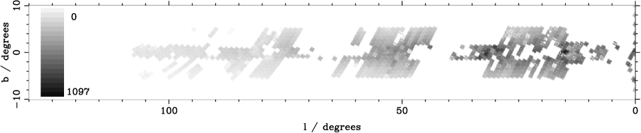
Figure 15: K–band star counts in the UKIDSS GPS produced by the query given in Section 4.2.4. The scale bar is in units of stars per square arcminute.

4.2.5 Optical/infrared selection of QSO candidates

Usage U2 in Appendix A requires two selections: (i) a set of point sources satisfying certain optical/infrared colour cuts; and (ii) a 1 in $10^{4}$ sampling of all point sources without those colour cuts. Both are easily achieved in SQL – the availability of the view lasPointSource is particularly convenient. The following query provides selection (i):

SELECT psfMag_i-psfMag_z    AS imz,
       psfMag_z-j_1AperMag3 AS zmj,
       psfMag_i-yAperMag3   AS imy,
       ymj_1Pnt             AS ymj
FROM   lasPointSource        AS s,
       lasSourceXDR5PhotoObj AS x,
       BestDR5..PhotoObj     AS p
WHERE
/* Join predicates: */
       s.sourceID   = x.masterObjID AND
       x.slaveObjID = p.objID       AND
       x.distanceMins < 1.0/60.0    AND
/* Select only the nearest primary SDSS
   point source crossmatch: */
       x.distanceMins IN (
         SELECT MIN(distanceMins)
         FROM   lasSourceXDR5PhotoObj
         WHERE  masterObjID = x.masterObjID AND
                sdssPrimary = 1             AND
                sdssType    = 6
       ) AND
/* Remove any default SDSS mags: */
       psfMag_i > 0.0 AND
/* Colour cuts for high-z QSOs from
   Hewett et al. (2006) and Venemans
   et al. (2007): */
       psfMag_i-yAperMag3 > 4.0 AND
       ymj_1Pnt           < 0.8 AND
       psfMagErr_u > 0.3 AND
       psfMagErr_g > 0.3 AND
       psfMagErr_r > 0.3
/* UKIDSS DR2 rows returned: 12
   Execution time:           19m 56s  */

where the colour cuts have been determined with reference to Hewitt et al. (2006) and Venemans et al. (2007). In fact, usage example U2 is somewhat unrealistic in that the ‘legacy’ SDSS lacks the depth to detect QSOs having $z\sim 7$ as illustrated in Venemans et al. (2007); optical drop–out techniques (see later) or deeper optical data are needed for the most highly redshifted QSOs. Furthermore, some contamination from differently deblended sources and poorly photometered sources near very bright stars is present in exactly the position where the high redshift QSO locus is expected to lie. However the SQL provided here serves at least to illustrate how to ask this kind of question in the WSA; moreover, it produces a list of a dozen candidates which is a viable number for closer scrutiny (e.g. inspection of image thumbnails and subsequent spectroscopic follow–up).

For selection (ii), removing the colour cut predicates and adding the predicate ... AND (sourceID%10000)=0 will select one in every $10^{4}$ sources randomly scattered over the survey area (the “%” modulo operator returns the remainder of the number on the left after dividing by that on the right). This is because sourceID is assigned sequentially in the source merging procedure and for large increments this attribute is not strongly correlated with position. The results are illustrated in the two–colour diagram in Figure 16 (1 in 10 sources plotted from UKIDSS DR2 cross–matched with SDSS DR5 rather than a 1–in–$10^{4}$ sampling).

Figure 16: Two–colour diagram (cf. Figure 5 of Hewitt et al. 2006) illustrating the principal colour space of optical/infrared QSO candidate selection (see Section 4.2.5).

4.2.6 A wide–area, shallow galaxy catalogue

Usage example U6 in Appendix A specifies the selection of a galaxy catalogue with full optical/infrared photometry to K=18.4 from the intersection of the UKIDSS LAS and SDSS optical survey. In the following example, we further extend this usage mode to extract redshift information from SDSS spectroscopy, and compute absolute magnitudes M_K via an Einstein–de Sitter cosmological distance modulus with Hubble constant $H_{0}=75$ km s^-1Mpc^-1, all in SQL. The nearest crossmatch between the LAS and SDSS with a matching tolerance of 2″ is selected:

SELECT s.ra as alpha, s.dec as delta,
/* Remove Galactic foreground reddening: */
       (petroMag_u-extinction_u)     AS u,
       (petroMag_g-extinction_g)     AS g,
       (petroMag_r-extinction_r)     AS r,
       (petroMag_i-extinction_i)     AS i,
       (petroMag_z-extinction_z)     AS z,
       (yPetroMag-ay)                AS y,
       (j_1PetroMag-aj)              AS j,
       (hPetroMag-ah)                AS h,
       (kPetroMag-ak)                AS k,
       z.z                           AS redshift,
       (modelMag_g-extinction_g) -
        (modelMag_r-extinction_r)    AS gmr,
       (yAperMag3-ay)-(kAperMag3-ak) AS ymk,
       (modelMag_u-extinction_u) -
        (modelMag_g-extinction_g)    AS umg,
/* Einstein-de Sitter cosmology distance modulus
   (note no K-correction, no evolution correction,
    and no internal extinction):  */
       (kPetroMag-ak) - 25 - 5*(
        LOG10(2*2.998e5*(1+z.z-SQRT(1+z.z))/75)
       ) AS M_K
FROM   lasExtendedSource AS s,
       lasSourceXDR5PhotoObj AS x,
       BestDR5..PhotoObj AS p,
       BestDR5..SpecObj AS z
WHERE
/* Join criteria:   */
       z.specObjID=p.specObjID    AND
       s.sourceID = x.masterObjID AND
       p.objID = x.slaveObjID     AND
       x.distanceMins IN (
       SELECT MIN(distanceMins)
       FROM   lasSourceXDR5PhotoObj
       WHERE  masterObjID = x.masterObjID AND
              distanceMins < 2.0/60.0
       ) AND
/* Dereddened magnitude cut as specified:  */
       (kPetroMag-ak) BETWEEN 0.0 AND 18.4 AND
       yPetroMag > 0  AND
       modelMag_u > 0 AND
       modelMag_g > 0 AND
       modelMag_r > 0 AND
/* Exclude any non spectroscopic redshift
   objects for a clean sample: */
       z.z BETWEEN 0.01 AND 0.15 AND
       z.zWarning=0
/* UKIDSS DR2 rows returned: 8,086
   Execution time:           05m 13s  */

In Figure 17 we plot M_K (as a proxy for total stellar mass) versus (u$-$g) which shows a bright red clump of ellipticals along with a sequence of fainter, bluer star–forming and/or spiral galaxies and finally yet fainter, bluer dwarfs.

Figure 17: Absolute–magnitude versus colour plot for a wide–area, shallow galaxy catalogue extracted using the query in Section 4.2.6 which trawls the UKIDSS LAS–DR2 and SDSS–DR5 crossmatch (see text).

Spatial sampling of selections from base table lasSource (or indeed any merged source table in the WSA) can be determined in several ways. The simplest method (e.g. for making an areal coverage plot) is to use the central positions of the frame sets available in lasMergeLog:

SELECT ra,dec
FROM   lasMergeLog
WHERE  j_1mfID > 0 AND
       hmfID   > 0 AND
       kmfID   > 0
/* UKIDSS DR2 rows returned: 6,242
   Execution time:           00m 04s  */

where the predicates require coverage in passbands JHK, but not necessarily Y, as is the case in view lasExtendedSource for example. The size of each frame set in the LAS is the size of one WFCAM detector, or 13.65 arcmin. Figure 18 shows the area covered by plotting squares of this size at each co-ordinate pair returned by the query.

Figure 18: Areal coverage of the galaxy catalogue selection described in Section 4.2.6.

More sophisticated functionality is provided via use of Hierarchical Triangular Mesh (HTM; Kunszt et al. 2000) indices which are available as attribute htmID where an equatorial RA,Dec pair are present in most WSA tables. For example, the set of HTM triangles covering a given selection to a given HTM level (see Kunszt et al. 2000) can be obtained using the SQL DISTINCT function along with division by an integer power $N$ of 4 to mask to the $(20-N)^{\rm TH}$ level where the WSA uses 20–level indexing by default:

SELECT DISTINCT(htmID/POWER(4,20-12))
FROM   lasSource
WHERE  ...

will return the identifiers of the HTM triangles at level 12 (areas between 0.86 and 1.8 square arcmin) covered by the LAS merged source table for the given predicates. Libraries of various routines for the manipulation and translation of spatial co-ordinates an associated HTM indices are are available online⁷. Note that the areal coverage maps returned by any of these queries are not the maps of survey depth that would be needed to compute survey volume corrections.

4.2.7 Infrared colour–selected sources that are optical drop–outs

Usage U1 in Appendix A requires non–detection in optical (iz) passbands for an infrared colour–selected sample of point sources as cool, substellar candidates (see, for example, Kendall et al. 2007). One could envisage this being achieved within the archive by automatically placing apertures in optical images (i.e. SDSS pixel data) at positions having infrared detections. In fact, it is much simpler to use the cross–neighbour functionality, requiring non–detection in the optical above a certain limit within a given radius of an infrared source. In this way it is possible to make a manageable candidate list in a single SQL SELECT statement. In U1, it is envisioned that the user develops the query for a rare object search by refining the search predicates. The starting point would be as follows:

SELECT COUNT(*)
FROM   lasSource
WHERE
/* Colour cuts for mid-T & later: */
       ymj_1Pnt > 0.5 AND
       j_1mhPnt < 0.0 AND
/* Source not detected above 2sigma within
   1" in SDSS-DR5 i’ or z’:                */
       sourceID NOT IN (
       SELECT masterObjID
       FROM   lasSourceXDR5PhotoObj AS x,
              BestDR5..PhotoObj     AS p
       WHERE  p.objID = x.slaveObjID   AND
              (psfMagErr_i < 0.5       OR
               psfMagErr_z < 0.5)      AND
              x.distanceMins < 1.0/60.0
        ) AND
/* Use only frame sets overlapping with
   SDSS-DR5:                            */
       frameSetID IN (
       SELECT DISTINCT(frameSetID)
       FROM   lasSource             AS s,
              lasSourceXDR5PhotoObj AS x
       WHERE  s.sourceID = x.masterObjID
       )
/* UKIDSS DR2 rows returned: 1 (count=46,141)
   Execution time:           16m 52s  */

which counts 46,141 candidates in the UKIDSS DR2 cross–match with SDSS–DR5. The first two predicates simply apply a colour cut based on prior knowledge of the objects being sought. The third predicate involves a subquery to exclude any object that has an optical counterpart above the specified limit ($2\sigma$) in the SDSS, and a further nested subquery to only use the nearest optical cross–match within 1″. Finally, a predicate subquery specifies that only LAS frame sets that contain SDSS cross–matches should be used in this search, since if any LAS imaging data are outwith the area covered by the SDSS, they must be excluded since all infrared sources in those regions would be counted as optical non–detections.

Clearly, $\sim 4.6\times 10^{4}$ candidates is an impractically large list for any useful purpose. The predicates need to be expanded to reduce the list of unwanted and spurious sources prior to a more intensive inspection of image thumbnails or indeed spectroscopic follow–up on large aperture facilities. Addition of the following predicates:

/* Unduplicated or primary duplicates only: */
        (priOrSec = 0 OR priOrSec = frameSetID) AND
/* Generally good quality: */
        yppErrBits   < 256 AND
        j_1ppErrBits < 256 AND
        hppErrBits   < 256 AND
/* Point-like morphological classification: */
        mergedClass=-1 AND
        mergedClassStat BETWEEN -3.0 AND +3.0 AND
/* Reasonably circular images in YJH: */
        yEll   < 0.35 AND
        j_1Ell < 0.35 AND
        hEll   < 0.35 AND
/* IR pairs within 0.5 arcsec: */
        j_1Xi  BETWEEN -0.5 AND +0.5 AND
        j_1Eta BETWEEN -0.5 AND +0.5 AND
        hXi    BETWEEN -0.5 AND +0.5 AND
        hEta   BETWEEN -0.5 AND +0.5 AND
/* YJ measured to 5 sigma and H to 4sigma: */
        yAperMag3Err   < 0.20 AND
        j_1AperMag3Err < 0.20 AND
        hAperMag3Err   < 0.25
/* UKIDSS DR2 rows returned: 1 (count=25)
   Execution time:           00m 48s  */

reduces the number of candidates to 25. The first predicate limits the search to unique objects where duplicates exist in overlap regions; the next set makes cuts on quality error flags; the next limits the search to point–like, circular sources making generous allowance for noisy, high ellipticities at low signal–to–noise; the penultimate predicate set restricts the selection to YJH pairs within 0.5″ boxes (the LAS pairing criterion is a generous 2.0″ – e.g. Table 4). All the predicates on attributes common to all passbands are applied across the relevant filter passbands (YJH) to limit the sample selection to those sources appearing in all three. Substituting SELECT COUNT(*) with

SELECT dbo.fIAUnameLAS(ra,dec),
       yAperMag3,
       ymj_1Pnt,ymj_1PntErr,
       j_1mhPnt,j_1mhPntErr

and including ORDER BY ra at the end of the query yields the results shown in Table 5. Note the syntax and use of the function fIAUnameLAS() to automatically output IAU standard names for any target. The candidate sample produced by the full query includes spectroscopically confirmed T dwarfs discussed in Lodieu et al. (2007b) and references therein.

Table 5: Candidate T–type brown dwarfs extracted from the UKIDSS LAS at Data Release 2 using the example query given in Section 4.2.7. The final column indicates the assigned spectral type (if known) from follow–up observations as reported in Warren et al. (2007b) for ULAS J0034 and Lodieu et al. (2007b) otherwise.

Candidate name	Y	Y$-$J	$\sigma_{\rm Y-J}$	J$-$H	$\sigma_{\rm J-H}$	Sp. type
ULAS J002422.93+002247.9	19.604	1.441	0.170	$-$0.093	0.174	T4.5
ULAS J003402.77–005206.7	18.905	0.769	0.130	$-$0.398	0.234	T8.5
ULAS J013738.55+011808.0	19.497	0.762	0.168	$-$0.013	0.231
ULAS J020331.51+012350.8	19.276	0.663	0.157	$-$0.001	0.219
ULAS J020336.94–010231.1	19.056	1.014	0.109	$-$0.284	0.132	T5.0
ULAS J021127.17+011606.1	19.226	0.647	0.124	$-$0.016	0.198
ULAS J022200.43–002410.5	19.734	1.084	0.151	$-$0.033	0.164
ULAS J024641.36+011800.5	19.767	0.615	0.203	$-$0.072	0.271
ULAS J024642.92+011628.9	19.685	0.880	0.169	$-$0.194	0.214
ULAS J025321.88+012319.8	19.961	0.726	0.192	$-$0.052	0.256
ULAS J030135.17+011903.8	19.524	0.685	0.165	$-$0.160	0.254
ULAS J083554.96–012556.6	18.942	0.695	0.110	$-$0.123	0.189
ULAS J084719.65–012701.2	19.206	0.551	0.146	$-$0.052	0.250
ULAS J093956.86–012109.7	19.327	0.638	0.126	$-$0.154	0.249
ULAS J094806.06+064805.0	20.030	1.177	0.158	$-$0.709	0.230	T7.0
ULAS J100513.82–003704.2	19.660	0.758	0.131	$-$0.004	0.228
ULAS J100759.90–010031.1	19.818	1.146	0.136	$-$0.119	0.195	T5.5
ULAS J115038.79+094942.8	19.588	1.012	0.139	$-$0.751	0.222
ULAS J115811.10+094236.1	19.899	0.550	0.186	$-$0.003	0.226
ULAS J131346.93+075451.8	20.238	0.992	0.196	$-$0.189	0.249
ULAS J145514.50+061655.8	20.163	0.784	0.229	$-$0.006	0.257
ULAS J150508.56+061547.1	19.871	0.690	0.161	$-$0.080	0.268
ULAS J155120.90+075159.5	19.121	0.539	0.104	$-$0.182	0.234
ULAS J223132.02+012334.5	19.519	0.517	0.185	$-$0.095	0.272
ULAS J224238.02+011804.3	19.499	0.547	0.174	$-$0.013	0.259

5 Conclusion

We have described the WFCAM Science archive (WSA), which is the end point in the data flow of UKIRT WFCAM data in the VISTA Data Flow System, and the primary point of access for users of survey science products, especially those of the United Kingdom Infrared Deep Sky Survey (UKIDSS). In particular, we have described:

• how the top–level requirements and typical usage modes informed the design of the WSA;

• the arrangement of survey data in terms of a set of related tables;

• the implementation of the archive within a commercial relational database management system;

• the curation procedures employed to create science–ready survey catalogues from standard pipeline–processed products;

• example real–world astronomy usage modes along with typical results.

The WSA is the prototype science archive for the VISTA surveys, and the design of the VISTA Science Archive will follow closely that described here.

6 Acknowledgements

Many people have contributed to the development of the WFCAM Science Archive. We would like to thank especially our colleagues in the Sloan Digital Sky Survey science archive project: Alex Szalay, Jan Vandenberg, Maria Nieto–Santisteban, Peter Kunszt, Tamas Budavári, and Ani Thakar at Johns Hopkins University, and Jim Gray from Microsoft Research, for all their advice during the design and implementation stages. We thank Microsoft also for providing software via the Microsoft Development Network Academic Alliance, and eGenix for providing a free, non–commercial licence for Python middleware. We would like to acknowledge help and support from the following individuals: Luc Simard, Frossie Economu, John Lightfoot, Tim Jenness, Andy Vick, Dave Lunney, Mark Casali, Mike Irwin, Jim Lewis, Peter Bunclark, Richard McMahon, Martin Hill, John Taylor, Mark Holliman, Jonathan Dearden, and Horst Meyerdierks. Eclipse Computing of Ayrshire have been unfailing in their supply of test equipment and final hardware solutions at highly competitive prices. The WSA team would like to acknowledge much helpful interaction with University of Edinburgh staff in the Schools of Physics and Informatics and the National e–Science Centre, and advice from Andy Knox of IBM concerning scalable hardware solutions. Finally, we would like to extend our thanks to Ian Carney of the Oracle Corporation for introducing us to the delights of entity–relationship modelling.

Financial resources for VISTA/WFCAM Science Archive development were provided by the UK Science and Technology Facilities Council (STFC; formerly the Particle Physics and Astronomy Research Council) via e–Science project funding for the VISTA Data Flow System. Operations resources, including provision for hardware, are provided in the main by the STFC, but we would also like to acknowledge significant contributions to hardware funding from University of Edinburgh sources.

This paper is dedicated to our colleague and friend Jim Gray.

Appendix A Twenty usages of the WFCAM Science Archive

Here we reproduce the typical usage modes of the WSA that were developed in collaboration with the UKIDSS user community during the design phase of the project (more details are available online):

U1: Count the number of sources in the LAS which satisfy the colour constraints (Y–J) $>1.0$, (J–H) $<0.5$ where SDSS iz flux limits at the same position are less than 2$\sigma$. User then refines the query as necessary to give a reasonable number of candidates. When satisfied, the user requests a list, selecting output attributes from those available for the LAS, and finder charts in JHK for each object.

U2: List all star-like objects with izYJHK SDSS/UKIDSS–LAS colours consistent with the colours of quasars at redshifts $5.8<z<7.2$ or $z>7.2$ (user specifies cuts in colour space). Return plots of (i–z) versus (z–J) and (i–Y) versus (Y–J) with these sources plotted in a specified symbol type, with 1 in every 10,000 other stellar sources plotted as points.

U3: For a given cluster target in the UKIDSS GCS, make a candidate membership list via selection of stellar sources in colour–magnitude, colour–colour and proper motion space. Cross–correlate the candidate list against a user–supplied catalogue of optical/near–infrared detections in the same region.

U4: From the UKIDSS LAS, provide a list of all stellar objects that have measured proper motions greater than 5x their estimated proper motion error; additionally give a count of all stellar objects that are unpaired between the two epochs of the LAS observations with specified conditions on image quality flags. User then refines these conditions to produce a manageable list of very high proper motion candidate stars. Return finder charts in JHK for all candidates.

U5: From the UKIDSS DXS & UDS, construct galaxy catalogues. User selects all non-stellar sources satisfying quality criteria. User also requires the spatial sampling of this catalogue. Cross-correlate the galaxy catalogues against user-supplied optical catalogue in the same region.

U6: From the UKIDSS LAS, construct a galaxy catalogue for all non-stellar sources satisfying K $<18.4$ and given quality criteria; return full photometric list from SDSS & UKIDSS: ugrizYJHK. User also requires the spatial sampling of this catalogue.

U7: From the UKIDSS UDS, select a sample of galaxies with colours and morphology consistent with being elliptical galaxies. Provide a spatial mask to enable determination of sample characteristics. Provide a measure of the half-light radius for each galaxy.

U8: From the UKIDSS GPS, provide star counts in 10 arcmin cells on a grid in Galactic longitude and latitude; also provide a list of cells where there is any quality issue rendering that cell’s value inaccurate.

U9: From the UKIDSS GPS, provide a list of all sources that have brightened by a given amount in the K band.

U10: Provide a plot of g–J vs J–K for all point–like sources detected in the UKIDSS/LAS survey subject to quality constraints. User interacts with the plot to fit a straight line (g–J)=a+b(J–K) to the main sequence stars. Then find all UKIDSS/LAS sources with g-J$>$a+b(J-K), 4$>$g–J$>$–1, and 3$>$J–K$>$–1.

U11: Construct H2–K difference image maps for all frames within a specified subregion surveyed by the GPS.

U12: Find all galaxies with a de Vaucouleurs profile and infrared colours consistent with being an elliptical galaxy in the Virgo region of the UKIDSS LAS.

U13: Given input co-ordinates and a search radius (arbitrary system and reference frame) provide a list of all WFCAM observations ever taken that contain data in all or part of the specified area.

U14: Provide a list of point-like sources with multiple epoch measurements which have light variations $>$ 0.1 magnitudes in J, H or K.

U15: From any UKIDSS data, where multiple epoch measures exist for the same object, provide a list of anything moving more than X arcsec per hour.

U16: Provide a list of star–like objects that are 1% rare for the 3–colour attributes.

U17: For a given device in a tile, give me all images from the UDS corresponding to that frame, stacked in 10 day bins.

U18: Give me a true colour JHK image mosaic using frames in the LAS centred at given co-ordinates (arbitrary reference frame and system) with 2 degree width and rebinned so that the entire mosaic is returned as a 2048x2048 pixel image.

U19: Find all detected sources from all UKIDSS surveys within 3x the error boxes of a user supplied list of X–ray transient sources.

U20: For all sources in a user–supplied radio catalogue of HII regions in the GPS, return the Br–gamma surface brightness in an aperture of X arcsec

Appendix B Structured Query Language data retrieval fundamentals

The basic, general form of a Structured Query Language (SQL; Klein & Klein 2001) statement for data retrieval (i.e. a query statement) in an RDBMS is as follows:

SELECT column-1 [, column-2, ...]
FROM table-set-1 [, table-set-2, ...]
WHERE condition-1 [ AND|OR condition-2 ... N] (B1)

The column definition is generally a comma–separated list of attribute names from columns contained in the table set defined in the FROM clause, e.g. SELECT ra, dec, frameSetID ..., but great flexibility is available in SQL: expressions involving literal constants, mathematical functions and statistical aggregates are all possible:

SELECT ’hello world’ (B2)
SELECT ra/15.0 AS raHours, ... (B3)
SELECT AVG(COS(RADIANS(dec))), ... (B4)
SELECT COUNT(DISTINCT multiframeID), ... (B5)

are all legal WSA SQL SELECT expressions; example (B2) is a complete SQL statement that, insofar as SQL can be considered a programming language, demonstrates the classic first step in learning the programming syntax – it returns a results set consisting of one row having one column having the specified string constant value. A more detailed explanation of SQL SELECT is given online at the WSA website in the ‘SQL Cookbook’, while a complete description including all standard clauses and non–standard Microsoft SQL Server extensions is available elsewhere. Note that Microsoft SQL syntax is not case–sensitive – mixed upper and lower case is used in the examples in this paper for clarity only.

The table set definition in its simplest form consists of the name of a single table, e.g.

SELECT ra, dec, frameSetID
FROM dxsMergeLog (B6)

returns the equatorial co-ordinates of all frame sets in the UKIDSS DXS along with their unique identification numbers that have been assigned in the WSA curation procedure. Once again, great flexibility is afforded in SQL in the table set definition: table-set-N may be any expression that defines a tabular dataset, e.g. a table name, a view name, or even another SELECT statement. For example,

SELECT t.*
FROM (
SELECT ra, dec, frameSetID
FROM dxsMergeLog
) AS t (B7)

is an unnecessarily complicated, but nonetheless legal, SQL equivalent to statement B6 above (the nested SELECT is commonly known as a subquery in this context; note the use of the alias “t” to conveniently label the subquery rowset for references elsewhere in the statement).

By far the most common table set definition that a user will need when retrieving data via free–form SQL statements is a comma–separated list of related tables. With reference to the relational model in Section 2.4.3, Figure 4, consider the case where a user wishes to obtain a list of the required filters (WSA filter unique identifiers filterID and number of multi–epoch passes in that filter) for the UKIDSS programmes, along with generic information on each programme. Since all the relevant information is spread between tables Programme and RequiredFilters, a selection from those two is required:

SELECT t1.programmeID, t1.description, t2.*
FROM Programme AS t1, RequiredFilters AS t2 (B8)

This query, however, results in the cartesian product of the two tables rather than a union of associated rows. Most of the rows in the results set produced by B8 are of course meaningless, since all $N$ rows in Programme are joined, one by one, with all $M$ rows of in RequiredFilters resulting in $N\times M$ rows. In order to produce the selection required, a WHERE clause must be used to associate the related rows,

WHERE t1.programmeID = t2.programmeID (B9)

since any rows where programmeID is different in the two tables are not related. Generally speaking, when querying data across $N$ tables there should be at least $N-1$ WHERE clause filters associating related attributes across the tables. The attributes to use in filtering are easily determined using the WSA schema browser (see Section 3 in the main text). They are nearly always indexed primary keys in the RDBMS implementation so are highlighted and are at the top of each table’s attribute list. Moreover a foreign key reference is noted at the top of each table definition for every many–to–one relationship in the data model; referencing attributes are generally the ones to filter on in the WHERE clause of a join query. Implicit join queries are very common in normalised relational database (e.g. Section 4 in the main text). The RDBMS design is optimised for the normal form, required storage space is minimised, and query performance is optimised for speed.

Otherwise, the WHERE clause is simply a list of conditional statements linked by logical operators (usually AND). These conditions are known as predicates. Comparison predicates are common:

WHERE (ra/15.0 < 12.0 OR dec >=+35.0) AND filterID <> 3 (B10)

Other types of predicate are defined in SQL – again, see the WSA SQL Cookbook or other online guides to the language.

Finally, there are some powerful optional clauses available to the SELECT statement. An ORDER BY clause can be specified, which sorts the results set returned by the specified expression. For example,

SELECT ra, dec, frameSetID
FROM dxsMergeLog
ORDER BY ra ASC (B11)

returns the same rows as B6 but in order of increasing, i.e. ASCending, RA; specify DESC for descending order. Note that without an ORDER BY clause, the order in which rows are retrieved from an RDBMS is undefined and, moreover, generally unrepeatable – the order can change between two consecutive runs of the same query.

Furthermore, particularly useful for summarising the characteristics of data in very large tables is the GROUP BY optional clause. This, along with bulit–in aggregate functions, enables the user to produce summary quantities or statistics for large amounts of data arbitrarily grouped together on an expression involving one or more column names. The GROUP BY clause is best illustrated with a few examples.

SELECT filterID, COUNT(*) AS totalFrames
FROM Multiframe
GROUP BY filterID (B12)

is a simple example which returns a count of the number of frames in each of the different filters used in observing. Note the use of the aggregate function COUNT in B12 above. Queries involving GROUP BY will generally use such built–in aggregate functions, and this is a particularly powerful combination. Other aggregate functions are available including minimum/maximum (MIN/MAX), average (AVG), summation (SUM) and statistical aggregates, for example standard deviation (STDEV). A slightly more complicated example is

SELECT frameSetID, AVG(ra) AS meanRA,
AVG(dec) AS meanDec,
COUNT(*) AS numSources
FROM lasSource
GROUP BY frameSetID
HAVING AVG(dec) > 0.0 (B13)

which returns a list of all northern hemisphere frame sets in the UKIDSS LAS, their mean RAs/Decs and a count of the number of sources in each. Note the additional HAVING clause: just as SELECT may have a WHERE clause to filter rows in the table(s) specified in the FROM clause, GROUP BY may include a HAVING clause to filter rows in the table formed by the specified grouping.

References

- [ ] Abazajian, K., et al., 2004, AJ, 128, 502
- [ ] Abazajian, K., et al., 2005, AJ, 129, 1755
- [ ] Adelman–McCarthy, J.K., et al., 2007, ApJS, 172, 634
- [ ] Barrett, P., 1993, Annals of the Israel Phys. Soc., 10, 276
- [ ] Bertin, E. & Arnouts S., 1996, A&AS, 117, 393
- [ ] Bertin, E., Mellier, Y., Radovich, M., Missonnier, G., Didelon, P., Morin, B., 2002, In: Astronomical Data Analysis Software and Systems XI, eds. D.A. Bohlender, D. Durand, & T.H. Handley, A.S.P. Conf. Ser., 281, 228
- [ ] Bonifacio, P., Monai, S., Beers, T.C., 2000, AJ, 120, 2065
- [ ] Calabretta, M.R., Griesen, E.W., 2002, A&A, 395, 1077
- [ ] Casali, M., et al., 2007, A&A, 467, 777
- [ ] Claver, C.F., et al., 2004, In: Proceedings of the SPIE, 5489, 705
- [ ] Collins, R.S., Cross, N.J.G., Hambly, N.C., Mann, R. G., Read, M., Sutorius, E., Williams, P.M., Bond, I.A., 2006, In: Proceedings of the 15th meeting on Astronomical Data Analysis and Software Systems (ADASS), eds. C. Gabriel, C. Arviset, D. Ponz & E. Solano, ASP Conf. Ser., 351, 743
- [ ] Cross, N.J.G., et al., 2007, In: Proceedings of the 16th meeting on Astronomical Data Analysis and Software Systems (ADASS), in print
- [ ] Devereux, D., Abel, D.J., Power, R.A., Lamb, P.R., 2005, In: Proceedings of the 14th Astronomical Data Analysis and Software Systems (ADASS), eds. P. Shopbell, M. Britton, & R. Ebert, ASP. Conf. Ser., 347, 346
- [ ] Dye, S., et al., 2006, MNRAS, 372, 1227
- [ ] Emerson, J.P., 2001, In: The New Era of Wide Field Astronomy, eds. R. Clowes, A. Adamson & G. Bromage, ASP Conf. Ser., 232, 339
- [ ] Emerson, J.P., et al., 2004, In: Optimizing Scientific Return for Astronomy through Information Technologies, Proceedings of the SPIE, 5493, 401
- [ ] Emerson, J.P., et al., 2006, In: Observatory Operations: Strategies, Processes, and Systems. eds. D.R. Silva & R.E. Doxsey, Proceedings of the SPIE, 6270, 25
- [ ] Epchtein, N. et al., 1994, Ap&SS, 217, 3
- [ ] Foucaud, S., et al., 2007, MNRAS, 376, 20
- [ ] Gaessler, W., et al., 2004, In: Optical, Infrared and Millimeter Space Telescopes, Proceedings of the SPIE, 5496, 79
- [ ] Gray, J., Szalay, A.S., Thakar, A.R., Stoughton, C., Vandenberg, J., 2002, In: Virtual Observatories, Proceedings of the SPIE, 4846, 103
- [ ] Hambly, N.C., et al., 2001a, MNRAS, 326, 1279
- [ ] Hambly, N.C., Irwin, M.J., MacGillivray, H.T., 2001b, MNRAS, 326, 1295
- [ ] Hambly, N.C., et al., 2004a, In: Optimizing Scientific Return for Astronomy through Information Technologies, Proceedings of the SPIE, 5493, 423
- [ ] Hambly, N.C., et al., 2004b, In: Proceedings of the 13th Astronomical Data Analysis and Software Systems (ADASS), eds. F. Oschenbein, M.G. Allen & D. Egret, ASP Conf. Ser., 314, 137
- [ ] Hanisch, R.J., et al., 2001, A&A, 376, 359
- [ ] Hewett, P.C., Warren, S.J., Leggett, S.K., Hodgkin, S.T., 2006, MNRAS, 367, 454
- [ ] Irwin, M.J., et al., 2007, in preparation
- [ ] Kaiser, N., 2004, In: Proceedings of the SPIE, 5489, 11
- [ ] Kendall, T.R. et al., 2007, A&A, 466, 1059
- [ ] Klein, K.E., Klein, D., 2001, ‘SQL in a nutshell: a desktop quick reference’, O’Reilly & Associates
- [ ] Kleinmann, S.G. et al., 1994, Ap&SS, 217, 11
- [ ] Kunszt, P.Z., Szalay, A.S., Csabai, I., Thakar, A.R., 2000, In: Proceedings of the 9th meeting on Astronomical Data Analysis and Software Systems (ADASS), eds. N. Manset, C. Veillet, & D. Crabtree, ASP Conf. Ser., 216, 141
- [ ] Lane, K.P. et al., 2007, MNRAS, 379, 25
- [ ] Lawrence, A., et al., 2002, In: Survey and Other Telescope Technologies and Discoveries, Proceedings of the SPIE, 4836, 418
- [ ] Lawrence, A., et al., 2007, MNRAS, 379, 1599
- [ ] Lodieu, N., Hambly, N.C., Jameson, R.F., Hodgkin, S.T., Carraro, G., Kendall, T.R., 2007a, MNRAS, 374, 372
- [ ] Lodieu, N., et al., 2007b, MNRAS, 379, 1423
- [ ] Lodieu, N., et al., 2007c, MNRAS, 380, 712
- [ ] Lupton, R.H., Gunn, J.E., Szalay, A.E., 1999, AJ, 118, 1406
- [ ] O’Mullane, W., Budavári, T., Li, N., Malik, T., Nieto-Santisteban, M. A., Szalay, A.S., Thakar, A.R., 2005, In: Astronomical Data Analysis Software and Systems XIV eds. P. Shopbell, M. Britton, & R. Ebert, A.S.P. Conf. Ser., 347, 341
- [ ] Perryman, M.A.C., 2005, In: Astrometry in the Age of the Next Generation of Large Telescopes, eds. P.K. Seidelman & A.K.B. Monet, ASP Conf. Ser., 338, 3
- [ ] Schlegel, D.J., Finkbeiner, D.P., Davis, M., 1998, ApJ, 500, 525
- [ ] Skrutskie, M.F., et al., 2006, AJ, 131, 1163
- [ ] Stoughton, C., et al., 2002, AJ, 123, 485
- [ ] Szalay, A.S., Kunszt, P.Z., Thakar, A.R., Gray, J., Slutz, D., 2000, In: Proceedings of the 9th meeting on Astronomical Data Analysis and Software Systems (ADASS), eds. N. Manset, C. Veillet & D. Crabtree, ASP Conf. Ser., 216, 405
- [ ] Thakar, A.R., Szalay, A.S., Vandenberg, J.V., Gray, J., Stoughton, A.S., 2003a, In: Proceedings of the 12th meeting on Astronomical Data Analysis and Software Systems (ADASS), eds. H.E. Payne, R.I. Jedrzejewski & R.N. Hook, ASP Conf. Ser., 295, 217
- [ ] Thakar, A.R., Szalay, A.S., Kunszt, P.Z., Gray, J., 2003b, Comput. Sci. Eng., 5, 16 (astro–ph/0403020)
- [ ] Venemans, B.P., McMahon, R.G., Warren, S.J., Gonzalez–Solares, E.A., Hewett, P.C., Mortlock, D.J., Dye, S., Sharp, R.G., 2007, MNRAS, 376, 76
- [ ] Walton, N.A., Gonzalez–Solares, E., Dalla, S., Richards, A.M.S., Tedds, J.A., 2006, Astronomy & Geophysics, 47, 22
- [ ] Warren, S.J., 2002, In: Survey and Other Telescope Technologies and Discoveries, Proceedings of the SPIE, 4836, 313
- [ ] Warren, S.J., et al., 2007a, MNRAS, 375, 213
- [ ] Warren, S.J., et al., 2007b, MNRAS, in press
- [ ] York, D.G. et al., 2000, AJ, 120, 1579