The Physics of the Intergalactic Medium111Submitted to the Reviews of Modern Physics.
Abstract
Intergalactic space is filled with a pervasive medium of ionized gas, the Intergalactic Medium (IGM). A residual neutral fraction is detected in the spectra of Quasi-Stellar Objects at both low and high redshifts, revealing a highly fluctuating medium with temperatures characteristic of photoionized gas. The statistics of the fluctuations are well-reproduced by numerical gravity-hydrodynamics simulations within the context of standard cosmological structure formation scenarios. As such, the study of the IGM offers an opportunity to probe the nature of the primordial density fluctuations on scales unavailable to other methods. The simulations also suggest the IGM is the dominant reservoir of baryons produced by the Big Bang, and so the principal source of the matter from which galaxies formed. The detection of metal systems within the IGM shows that it was enriched by evolved stars early in its history, demonstrating an intimate connection between galaxy formation and the IGM. The author presents a comprehensive review of the current understanding of the structure and physical properties of the IGM and its relation to galaxies, concluding with comments on prospects for furthering the study of the IGM using future ground-based facilities and space-based experiments.
I INTRODUCTION
According to the Big Bang theory, the primordial hydrogen and helium created in the Universe first materialized in the form of an extremely hot ionized gas. By the time the Universe was three hundred thousand years old, adiabatic expansion cooling brought the temperature of the primordial plasma down until the hydrogen and helium recombined. The radiation last scattered at this time appears today as the Cosmic Microwave Background (CMB). The search for the IGM began well before the discovery of the CMB with an attempt by Field (1959a) to detect the hyperfine 21cm absorption signature from hydrogen along the line of sight to the extragalactic radio galaxy Cygnus A. Although no detection was made, combining the optical depth with the measured temperature of the CMB discovered in 1965 would have been sufficient to exclude the possibility that the Universe was closed by baryons, with an upper limit on the baryon density of only 20% of the closure density required for an Einstein-deSitter (flat) universe. 333This conclusion requires making the (at the time) reasonable assumptions that the hydrogen was all neutral and that the hyperfine structure levels of the hydrogen were in thermal equilibrium with the CMB.
Nearly coincident with the discovery of the CMB, however, a considerably improved measurement of the density of intergalactic neutral hydrogen was made. Soon after the discovery of the first Quasi-Stellar Object (QSO) Hazard et al. (1963); Schmidt (1963), Gunn and Peterson (1965) reported a small decrement in a QSO spectrum shortward of its Lyemission line. Attributing the decrement to the Lyresonance scattering of radiation from the QSO by intergalactic neutral hydrogen, Gunn and Peterson demonstrated that the cosmic mass density of neutral hydrogen was exceedingly smaller than the Einstein-deSitter density. In fact, it was far smaller than the spatially averaged hydrogen of all the stars in the Universe. If the Big Bang theory was correct, it meant either that galaxy formation was an extraordinarily efficient process, sweeping up all but a tiny residue of the primordial hydrogen, or that the gas was reionized.
These two themes, the detection of intergalactic gas through the 21cm signature in the radio or through Lyman resonance scattering lines in the optical or ultraviolet (UV), continue to dominate studies of the Intergalactic Medium (IGM). To date, almost all that is known about the structure of the IGM has been derived from optical and UV data. This situation is expected to change dramatically in the near future with the development of low frequency radio arrays like the LOw Frequency ARray (LOFAR)444http://www.lofar.org, the Murchison Widefield Array (MWA)555http://www.haystack.mit.edu/ast/arrays/mwa/, the Primeval Structure Telescope (PaST/21CMA) 666http://web.phys.cmu.edu/past/, the Precision Array to Probe the Epoch of Reionization (PAPER) 777http://astro.berkeley.edu/dbacker/eor/, and a possible Square Kilometre Array (SKA). 888http://www.skatelescope.org A primary science driver of these instruments is the direct imaging of the IGM prior to the completion of the Epoch of Reionization Madau et al. (1997). Most of this review focuses on the current understanding of the state of the IGM as determined from optical and UV measurements. The observations have relied almost exclusively on the spectra of QSOs, although IGM absorption features have also been detected in the spectra of Gamma-Ray Bursts (GRBs) Totani et al. (2006), and indeed played a key role in establishing the extragalactic character of some bursts Metzger et al. (1997).
Almost immediately after Gunn and Peterson publicized their finding, it was recognized that individual Lyabsorption features should appear from neutral hydrogen concentrated into cosmological structures Bahcall and Salpeter (1965); Wagoner (1967). Absorption features had in fact been detected in higher resolution QSO spectra, but these were identified with intervening ionized metal absorption systems Bahcall et al. (1968), as was expected if galaxies had hot halos of ionized gas: the lines of sight to background QSOs were expected to pass through such hot halos and intercept any ionized gas clouds within them Bahcall and Spitzer (1969). The features, however, were uncomfortably common, hinting at a class of unknown structures not associated with galaxies. The Lyresonance line features continued to prove elusive until 1971, when Lynds (1971) recognized several absorption features shortward of the Lyemission line of a QSO as Lylines999These are not true absorption features involving the net destruction of a photon, but the scattering out of the line of sight of resonance line photons. arising in a population of discrete absorption systems also showing metal features. The Lylines form a plethora of distinct absorption features in the spectra of high redshift QSOs; they are collectively known today as the Lyforest.
The properties of the Lyforest came under increasing scrutiny, with the first systematic survey conducted several years later by Sargent et al. (1980), convincingly demonstrating through the homogeneity of the observed properties of the absorbers their intergalactic origin, as opposed to clouds ejected by the QSOs observed. Although limited by the resolution of the spectrograph, the measured velocity widths of the Lyfeatures corresponded to gas temperatures of a few to several K, characteristic photoionization temperatures for gas of a primordial composition, for which there is no significant cooling by metals. The number of features per comoving length was shown to increase with redshift, demonstrating that the systems were evolving Young et al. (1982).
The past decade has witnessed a dramatic improvement in precision studies of the Lyforest with the advent of 8–10 m class telescopes, particularly the Keck 10-m and the 8.2m Very Large Telescope (VLT). For the first time, the individual absorption features in the Lyforest were spectroscopically resolved over their full range. Velocity widths of are typical. The neutral hydrogen column densities of the absorbers range from roughly . The highest column density systems, the Damped LyAbsorbers (DLAs), are of particular interest for galaxy formation, as they are suspected of containing the neutral gas that formed the bulk of the stars in present day galaxies.
As the number per length of absorption systems increases along a line of sight with increasing redshift, so does the mean flux decrement in a background QSO spectrum due to Lyscattering. The QSO spectra measured as part of the Sloan Digital Sky Survey (SDSS) 101010http://www.sdss.org show a rapid rise in the flux decrement at , suggesting that the epoch of H reionization may lie not far beyond . Many of the hydrogen features also show absorption lines from metals, including carbon, silicon, nitrogen, oxygen, magnesium, iron and others. The abundances of the metals, however, are at most about 10% of solar at low redshifts, and as low as 1% at high redshifts, indicating that the absorption systems are comprised largely of primordial material. The primordial nature of the gas received further important confirmation in 1994 with the discovery by Jakobsen et al. (1994) of intergalactic helium using the Hubble Space Telescope (HST) through the detection of He Lyabsorption.
Because the baryons in the IGM are detected only though their absorption signatures, the physical structures that give rise to the features must be modeled. Early models characterized the systems as discrete clouds of gas, with most of the focus on either clouds pressure-confined by a hot medium Sargent et al. (1980), or gravitationally confined in a dark matter halo Ikeuchi (1986); Rees (1986). At the time it was believed that the absorption systems accounted for only a few percent of the baryons produced in the Big Bang, much like galaxies, their visible counterparts. A paradigm shift in the models occurred in the mid 1990s. Measurements of coincident absorption features along neighboring lines of sight suggested sizes of tens to hundreds of kiloparsecs for the absorbers Smette et al. (1992); Bechtold et al. (1994); Dinshaw et al. (1997), much larger than expected for clouds confined by pressure or dark matter halos. A radical transformation in the understanding of the nature and structure of the IGM was initiated by numerical simulations of cosmological structure formation. Today essentially all of the baryons produced in the Big Bang are believed to have undergone the same gravitational instability process initiated by primordial density fluctuations that was responsible for the formation of galaxies. The computation of the structure of the IGM has been converted into an initial value problem similar to that of the CMB fluctuations. Fluctuations in the CMB are solved for by following the gravitational instability growth of a postulated spectrum of primordial dark matter density fluctuations. The growth of structure in the IGM is now treated as the nonlinear extension of these computations. The result is a network of filamentary structures, the so-called “cosmic web” Bond et al. (1996). The Lyforest is believed to be a signature of the cosmic web. Early simulations broadly reproduced the statistics of the Lyforest spectacularly well Cen et al. (1994); Petitjean et al. (1995); Zhang et al. (1995); Hernquist et al. (1996); Zhang et al. (1997); Theuns et al. (1998). An immediate conclusion was that at , some 90% of the baryons produced in the Big Bang are contained within the IGM, with only 10% in galaxies, galaxy clusters or possibly locked up in an early generation of compact stars.
Soon after the discovery of intervening absorption features, it was recognized that they provided potentially powerful tests of fundamental properties of the Universe. The split in the fine structure lines of the metals was used to set constraints on the variability of the fine structure constant Bahcall et al. (1967). A bunching of absorption features near (now known to be fortuitous), gave rise to the (re)introduction of a cosmological constant to account for the numerous features as multiple images due to lensing Petrosian et al. (1967). The expected primordial composition of the IGM offered the potential of placing constraints on the photon-to-baryon ratio of the Universe through measurements of the intergalactic deuterium abundance. More recently, the success of the models has inspired attempts to exploit the Lyforest as a new means to constrain cosmological structure formation models and obtain stringent constraints on the cosmological parameters.
The description of the IGM by the simulations, however, is far from complete. There remain many unsolved problems. The current simulations do not reproduce all the observed properties of the IGM. The absorption lines are predicted to be substantially narrower than measured. This likely stems from the principal outstanding missing piece of physics, the reionization of the IGM. Not only must hydrogen be ionized, but helium as well. The ionization heats the gas through the photoelectric effect. Detailed radiative transfer computations are required to recover the temperatures, for which there is still limited success. The sources of the reionization and the epochs of reionization, both of hydrogen and helium, are still not firmly established. The origin of the metal absorption systems in the diffuse IGM is still unknown, although it is widely expected they were deposited by winds from galaxies, possibly driven by intense episodes of star formation. As such, the metal absorption lines in principle offer an important means of studying the history of cosmic star formation. Most fundamentally, the relation of the IGM to the galaxies that form from it is still mostly unknown, but offers perhaps the most exciting prospects for new research directions.
The purpose of this review is to describe the progress made in the understanding of the origin of structure within the IGM, with a view to presenting the underlying physics that determines the structure. An understanding of the physics is necessary for future progress. The past decade has revealed the IGM to be a complex dynamical arena involving interactions between the IGM gas, galaxies and QSOs. It is becoming increasingly apparent that the separation of these systems into distinct and isolated entities is an artificial construct. Galaxies and QSOs originated from the IGM, and their radiation and outflows impacted upon it. Any complete understanding of the origin of these systems requires a unified treatment. In this way, the IGM resembles the interstellar medium of disk galaxies in which the gaseous component is intimately linked to the stars and their evolution and impact. Interpreting the increasingly refined observations requires detailed modeling, which relies on large-scale numerical computations involving gas, radiative processes, and gravity. The physics involved is intermediate in complexity between that of the CMB and galaxy formation, rendering the IGM a bridge between these extreme scales of cosmological structure formation. Unraveling the processes that led to the formation and structure of the IGM may thus serve as a crucial step in the solution of the much more involved problem of galaxy formation.

A search of the literature for papers on the IGM since the Gunn & Peterson (1965) measurement produces close to 6000 references.111111Based on a boolean search of the Astrophysics Data System abstract service (adsabs.harvard.edu) for all refereed papers with abstracts or keywords containing “(intergalactic and medium) or (quasar and absorption and line).” Reionization papers are selected as the subset discussing the reionization of the IGM or the subsequent ionization structure of the IGM. While this review does not have the space to describe the observational methods used to measure the IGM, it should be recognized that progress in the understanding of the properties of the IGM is indebted to advances in observational techniques. This is well illustrated by a plot of the number of refereed publications in the field against time. Periods of relatively steady output are punctuated by four leaps. The first occurs at the end of the 1960s and beginning of the 1970s with the introduction of image tube spectrographs coupled with integrating television systems for photon counting Boksenberg (1972); Morton (1972), which greatly facilitated the taking of spectra. The next occurs in the mid-1970s with the development of x-ray astronomy following the launch of the UHURU satellite in 1970 and the recognition that galaxy clusters contain an extended and pervasive medium of hot, radiating gas Kellogg et al. (1973); Lea et al. (1973). Another sharp rise occurs in the early 1990s following the launch of the Hubble Space Telescope in 1990, the installation of EMMI and its echelle spectroscope on the New Technology Telescope (NTT) D’Odorico (1990), and the delivery of the HIRES spectrometer Vogt et al. (1994) to the Keck telescope. The fourth occurred in 2000 with the introduction of the UV and Visible Echelle Spectrograph (UVES) to the Very Large Telescope (VLT) D’Odorico et al. (2000), the launch of the Far Ultraviolet Spectroscopic Explorer (FUSE) Moos et al. (2000), and the beginning of operations of the Sloan Digital Sky Survey York et al. (2000). The latter in particular triggered a surge of activity in reionization studies following the discovery of high redshift QSOs () with spectra indicating a rapid rise in the effective optical depth of the IGM to Lyphotons, hinting that the Epoch of Reionization was being approached Becker et al. (2001); Fan et al. (2002). This is indicated by a rise in IGM reionization papers in Fig. 1, a trend which continues today, fueled in part by the growing interest in the influence of reionization on the CMB fluctuations measured by the Wilkinson Microwave Anisotropy Probe (WMAP) Kogut et al. (2003). The next major leap may well come from the anticipated radio measurements.
The rapidly rising tide of IGM studies has brought along with it several reviews. This is fortunate, as it is impossible in a single review to cover all areas thoroughly today. Early reviews of the QSO absorption line literature, now largely historical, were provided by Strittmatter and Williams (1976) and Weymann et al. (1981). Rauch (1998) and Bechtold (2003) provide reviews of the Lyforest that are still largely up-to-date in the sense that most of the topics currently engaging the community are treated, with developments since mostly improvements in accuracy and in the details of the numerical models. Reviews of the low redshift IGM are provided by Shull (2003) and Stocke et al. (2006b). Wolfe et al. (2005) have reviewed the current understanding of Damped LyAbsorbers, an absorber class of special concern as it represents the closest link to the gaseous component forming present day galaxies. A new series of reviews followed the recent explosion of activity on the reionization of the IGM in anticipation of the detection of the Epoch of Reionization (EoR) through its high redshift 21cm signature. An early review in this area is by Loeb and Barkana (2001). Since then, current observational and theoretical aspects of reionization have been exhaustively covered by Fan et al. (2006a), Furlanetto et al. (2006), and Barkana and Loeb (2007).
Rather than repeating the wide range of IGM phenomenology already covered by previous reviewers, I concentrate here on the physics underlying the structure of the IGM. One aim is to describe the physical underpinnings of current numerical simulations as required for future simulations to further progress. As observations are crucial for constraining any models, I begin by giving a broad overview of the current observational situation. The next section describes the physics of ionization equilibrium, followed by a discussion of the UV metagalactic background that maintains the ionization of the IGM. A brief review of early models of the Lyforest absorbers is then presented, followed by a discussion of current numerical models. The reionization of the IGM is then summarized along with means for its detection. This is followed by a discussion of the connection between galaxies and the IGM before concluding with observational and theoretical prospects for the future.
Unless stated otherwise, the cosmological parameters and are assumed for, respectively, the ratios of the present day matter density and the present day vacuum energy density to the current Einstein-deSitter density , a Hubble Constant of with (), and a baryon density of . These values are consistent within the errors with the current best estimates for a flat Universe based on CMB measurements using Year-5 WMAP data of , , , and Komatsu et al. (2008), or intergalactic measurements, giving O’Meara et al. (2006).
II Observations
II.1 Resonance absorption lines
The IGM is detected through the absorption features it produces in the spectrum of a background bright source of light (typically a QSO). The production of the absorption features is governed by the equation of radiative transfer through the IGM, conventionally expressed in terms of the specific intensity of a background radiation source.
The specific intensity is defined as the rate at which energy crosses a unit area per unit solid angle per unit time as carried by photons of energy traveling in the direction relative to some fiducial direction. The equation of radiative transfer for in a medium with attenuation coefficient is
| (1) |
Because of its use below, a radiative source term has been included through the emission coefficient , which describes the local specific luminosity per solid angle per unit volume emitted by sources. Normally the random orientation of atoms will ensure is isotropic, but not always, as for instance if the source includes a scattering term, so that a dependence on is included to account for the possibility of anisotropic sources. A central source like a QSO or galaxy will in fact generally radiate anisotropically.
In general, the attenuation of the radiation field is due both to the absorption of photons and their scattering out of the beam. The attenuation coefficient is then
| (2) |
where is the mass density of the medium, is the opacity, which expresses the absorption cross section per unit mass, is the number density of scattering particles of mean mass , and is the scattering cross section. In general, the scattering could arise from more than one type of particle, in which case would be replaced by a sum over particle species of density and cross section . In a static medium, is generally isotropic, but not always. As an example, the alignment of atoms in a strong magnetic field would absorb anisotropically. In a moving medium, an anisotropic contribution to the attenuation will be produced by the dependence of Doppler scattering on the relative motion of the radiation and the fluid.
The value of at any given time and position along the direction will be given by any incoming intensity at position at time , attenuated by intervening material at positions at the retarded times , along with contributions from sources at positions that emitted at the retarded times , followed by attenuation. The formal solution to Eq. (1) is then
| (3) |
as may be verified by direct substitution. In a uniformly expanding (or contracting) medium described by the scale factor , Eq. (1) must be modified to
| (4) |
where the frequency redshifts according to . The solution becomes
| (5) |
where , , and .
In the case of no intermediate sources, and the received intensity depends only on how the incident intensity is modified by the intervening gas. This is the situation for a single background source such as a QSO. The Lyman absorption features arise from the scattering of resonance line photons received from the background QSO through a medium of scatterers with number density . The frequency dependent scattering cross section for a scatterer at rest is given by the Lorentz profile121212SI units for electrostatic quantities throughout the text may be accommodated by including the square-bracketed quantity , where is the vacuum permittivity. Without the factor, the expressions correspond to the forms appropriate for cgs units.
| (6) |
where is the resonance line frequency, corresponding to the wavelength , of the transition between an upper level broadened by radiation damping to a sharp lower level (the ground state), is the damping width of the upper level, where and are the respective statistical weights of the lower and upper levels, is the upward oscillator strength, is the electric charge of an electron, and the electron mass.131313The Lorentz profile neglects the frequency dependence of the scattering cross-section far from line center. It does not, for example, recover the low frequency Rayleigh limit (). The profile, however, is fully adequate for all practical applications to the IGM. Small deviations may become detectable for broad absorption features such as Damped LyAbsorbers at high spectral resolution (Lee, 2003). Such deviations, however, would prove difficult to distinguish from the effects of density inhomogeneities in the absorbing gas and the associated gas velocities, except possibly in a statistical sense over many systems. The cross section is normalized according to
| (7) |
For in m, . For the Lyman series,
| (8) |
where is the quantum number of the upper state Menzel and Pekeris (1935). For the Lytransition, , and . For hydrogen Ly, Å and . For He Ly, is smaller by a factor of 4, and larger by a factor of 16.
In general, the atoms will not be at rest. At the very least they will generally undergo thermal motions described by a Maxwellian velocity distribution corresponding to their temperature . They may additionally take part in an ordered flow of velocity , but this may be accounted for by shifting the line center frequency to , to first order accuracy in , where is the line-of-sight velocity. In addition, there may be a disordered turbulent, or so-called microturbulent, component in some collapsed or shocked regions. Ignoring non-thermal velocities, the profile including thermal motions is found by convolving Eq. (6) with a Maxwellian. The result, which neglects additional frequency dependences far from line center, is the Voigt function
| (9) |
where is the ratio of the damping width to the Doppler width, and is the frequency shift from line center in units of the Doppler width with Doppler parameter
| (10) |
where is the mass of the scattering particle and is Boltzmann’s constant. A kinematic component such as microturbulence is often accounted for by adding in quadrature the characteristic kinematic velocity to the thermal component of the Doppler parameter
| (11) |
where is the thermal contribution from Eq. (10). An expansion approximation for the Voigt function in is provided by Harris (1948). Fast methods for arbitrary are described by Humlíček (1979), Humlíček (1982) and Shippony and Read (1993). Various evaluation methods are compared by Schreier (1992).
The resonance line scattering cross section is
| (12) |
where
| (13) |
is the Voigt profile, normalized to . For hydrogen Ly, . For He Ly, is larger by a factor of 8.
The intensity of the background QSO is attenuated by the factor , where Eq. (5) gives
| (14) |
For a homogeneous and isotropic background Universe expanding with scale factor , radiation emitted by the source at time and rest frame frequency , where is the resonance line frequency of a (rest frame) Lyman transition, will be scattered by the medium at epoch given by . Thus all of the received QSO intensity will be attenuated at the time at all observed frequencies in the range , or wavelengths in the range , where is the (rest frame) wavelength of the particular Lyman transition, producing a trough in the spectrum of the QSO. This is the Gunn-Peterson effect Gunn and Peterson (1965); Scheuer (1965). Intervening metal absorption, assuming solar abundances distributed uniformly throughout intergalactic space, would produce similar troughs Shklovskii (1964, 1965). The corresponding optical depth is given by noting that , where is the Hubble parameter at time . Changing the integration variable to and setting , it follows from Eq. (14) that, taking to denote the mean number density of particles in the lower state,
| (15) | |||||
after noting from Eq. (7) that . The Hubble parameter at redshift is related to the value of the Hubble constant today by , where Sargent et al. (1980); Peebles (1993). Here, is the mass density of the Universe expressed as a fraction of the Einstein-de Sitter critical density, and and are similar fractions arising from the curvature and vacuum energy contributions, respectively. They satisfy the identity . In the last line of Eq. (15), the result was scaled to the present day mean cosmic hydrogen density , where is the mass of a hydrogen atom and assuming a baryon density of (see § II.2.4 below) and cosmic helium mass fraction Peimbert et al. (2007), and to a Hubble Constant of (§ II.2.2 below). Eq. (15) is the inverse of the Sobolev parameter for a homogeneously and isotropically expanding medium, and was first derived in the context of cosmological hydrogen Lyphoton scattering by Field (1959b).
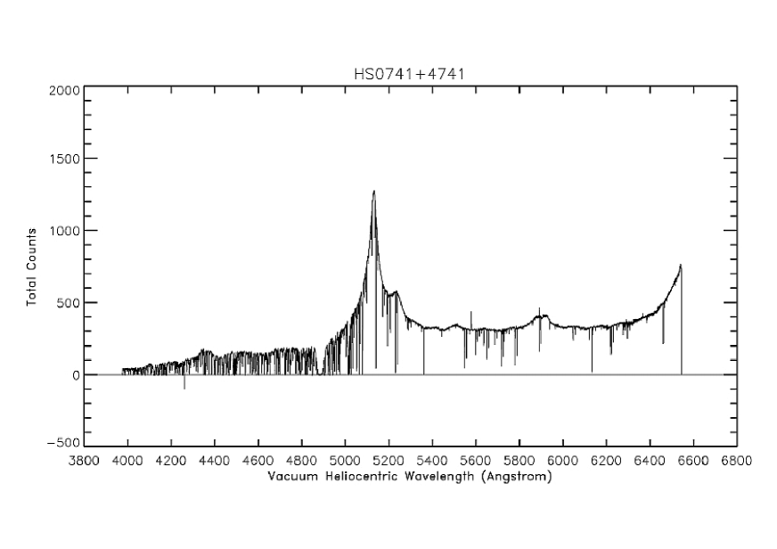
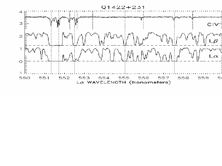
Observations show that in fact the IGM is not homogeneous, but that the baryons have coalesced, creating a fluctuating density field . The discreteness of the absorption lines measured in the spectra of high redshift QSOs suggests they originate in distinct localized regions. The resulting collection of absorption features, shown in Fig. 2, is known as the Lyforest. Denoting the centers of the absorbing regions by the positions , the optical depth becomes , where
| (16) |
Here, the integral has been localized to a region of width around , and , where corresponds to the epoch of coordinate in an expanding universe. The absorption features thus probe discrete spatial structures in the IGM. Expressing the optical depth as a sum of discrete absorption systems is, however, an approximation, as the intergalactic gas forms an evolving spatial continuum. Gas distributed over a wide spatial range, and even at different epochs, can therefore affect the same observed frequency . However, for , observations show the discrete absorber approximation provides a reasonably good description of the hydrogen Lyforest. Eq. (16) may be further simplified to
| (17) |
where
| (18) |
is the optical depth at line centre. Here, is the column density , and is averaged over the line of sight, weighted by the density. This may differ from when the temperature or large-scale macroscopic velocity field varies along the line of sight. Tabulations of and related atomic data for resonance lines for a variety of elements are available in the literature Morton (1991, 2000, 2003). For hydrogen Ly,
| (19) |

At redshifts , the blending of absorption lines makes it increasingly difficult to attribute the absorption to distinguishable systems. By , the individual lines have essentially all merged, forming in effect a Gunn-Peterson trough (though still not corresponding to a completely neutral IGM). Absorption features at intermediate redshifts not easily deblended into subcomponents may be characterized by an equivalent width . This is defined to be the width, expressed in units of wavelength, a square-well absorption feature with zero flux at its bottom must have to match the integrated area of the detected feature under the continuum:
| (20) |
For a Voigt profile, the equivalent width is related to the column density through the line-center optical depth according to
| (21) |
where
| (22) |
The relationship between the equivalent width and the column density is known as the “curve of growth.” For , the absorption profiles are well-approximated as Doppler in shape, corresponding to , and may be denoted more simply by . The function may be expressed as the power series Münch (1968)
| (23) |
For very optically thin lines (), , and the equivalent width is related linearly to the column density,
| (24) |
where has the dimension . Such features are said to lie on the “linear” part of the curve of growth.
For , better than 1% accuracy is provided by the asymptotic series Münch (1968)
| (25) |
For H Lyat a temperature K, deviates from the logarithmic approximation Eq. (25) by less than 10% for . Such features are said to lie on the “logarithmic” part of the curve of growth. They are also referred to as “saturated” lines, since an increase in the column density has only a small change on the shape of the absorption feature. The measurement of accurate column densities is notoriously difficult for these features, necessitating the search for higher order resonance lines on a more linear part of the curve of growth if accurate column densities are desired. On the other hand, the equivalent width is nearly directly proportional to the Doppler width, allowing an accurate determination of the Doppler parameter.
For very large values of , the Lorentzian radiation damping wings of the Voigt profile dominate the line profile, which in this limit is well approximated by . In this case, the equivalent width is given approximately by
| (26) |
Because of the square-root dependence on column density, this limit is referred to as the “square-root” part of the curve of growth. While the independence of the equivalent width on the Doppler width of the feature leaves poorly determined, the stronger dependence on the column density permits a more accurate determination of the column density from the equivalent width, or from line-profile fitting, than is possible for systems on the logarithmic part. The square-root approximation Eq. (26), however, is accurate only for very large values of . It is more than 25% too low for . Better than 1% accuracy is achieved for .
II.2 Absorption line properties
| Line parameters | Physical characteristics | |||||||
|---|---|---|---|---|---|---|---|---|
| Absorber class | (cm-2) | Size (kpc) | ||||||
| Ly forest | 15–60 | 15–1000(?) | -3.5 – -2 | 6.1 | 2.47 | |||
| LLS | – | -3 – -2 | 0.3 | 1.50 | ||||
| Super LLS | – | -1 – +0.6 | 0.03 | 1.50 | ||||
| DLA | ; | ; | (?) | -1.5 – -0.8 | ||||
| aApproximate ranges. Not well determined for most Lyman Limit Systems and super Lyman Limit Systems. |
| bValues not well constrained by direct observations. |
| cApproximate metallicity range, expressed as a logarithmic fraction of solar: . |
| dFor the following H column density and redshift ranges. For the Lyforest: and ; |
| for Lyman Limit Systems: and . The same evolution rate is adopted for super Lyman |
| Limit Systems. The evolution rate of Damped LyAbsorbers over the range is consistent with that of |
| Lyman Limit Systems, but poorly constrained by observations. |
II.2.1 Physical properties of absorption line systems
The absorption features comprising the Lyforest are broadly classified into three main types: Lyforest systems, Damped LyAbsorbers (DLAs), and Lyman Limit Systems (LLSs). The classification is based primarily on the physical origin of the features. The Lyforest systems, by far the most common, are generally well-fit by Doppler line profiles. The much rarer DLAs have sufficiently high hydrogen column densities that they show the radiation damping wings of the Lorentz profile, and require the Voigt line profile for accurate fitting. The intermediate LLSs have a sufficiently large column density to absorb photons with energies above the photoelectric edge, or Lyman limit. The classifications are not strictly exclusive. Damped absorbers of course produce Lyman Limit Systems. Lower column density Lyman Limit Systems will produce a Lyforest feature. For convenience, the features, however, are treated as distinct, corresponding typically to the column density ranges shown in Table LABEL:tab:absprops. Recently, a subclass of super Lyman Limit Systems (sLLSs) has been introduced, corresponding to systems with Wolfe et al. (2005).141414Although the SI system is used throughout this review, column densities are expressed with dimensions of to be consistent with the convention in the literature. These systems are convenient for statistical studies since their column densities are more easily determined than their lower column density counterparts because the damping wings begin to appear. They are sometimes also referred to as sub-damped absorbers, but there is an important physical distinction between them and the general class of DLAs: the hydrogen in the DLAs is essentially neutral, while the sLLSs are sufficiently penetrated by the UV metagalactic background as to be partially ionized. It is therefore reasonable to distinguish the DLAs as an entirely unique class of absorber.

A great number of surveys of QSO intervening absorption systems have been carried out, building up a large inventory of their statistical properties. Systematic surveys of the Lyforest were conducted by Weymann et al. (1979), Sargent et al. (1980), Bechtold (1994), Hu et al. (1995), Storrie-Lombardi et al. (1996), Kim et al. (2002a), Bechtold et al. (2002), and Tytler et al. (2004b). Surveys of Lyman Limit Systems were conducted by Sargent et al. (1989), Lanzetta et al. (1995b) and O’Meara et al. (2007). Surveys of Damped LyAbsorbers were conducted by Wolfe et al. (1986), Lanzetta et al. (1991), Lu et al. (1993), Lu and Wolfe (1994), Lanzetta et al. (1995b), Wolfe et al. (1995), Storrie-Lombardi and Wolfe (2000), Ellison et al. (2001), Ellison et al. (2002), Colbert and Malkan (2002), Akerman et al. (2005), Srianand et al. (2005), Rao et al. (2006) and Jorgenson et al. (2006). A radio survey of intervening absorption systems was carried out by Gupta et al. (2007). Surveys for galaxies associated with intervening absorption systems were conducted for galaxies associated with diffuse Lyabsorption systems at by Lanzetta et al. (1995a), Chen et al. (2005b), Morris and Jannuzi (2006), and Ryan-Weber (2006), with Damped LyAbsorbers by Chen and Lanzetta (2003), Cooke et al. (2005), and Cooke et al. (2006), and with metal absorption systems at by Tumlinson et al. (2005), Prochaska et al. (2006), Stocke et al. (2006a) and Kacprzak et al. (2008), and at by Adelberger et al. (2005).
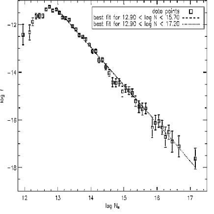
The neutral hydrogen column densities of the absorbers are measured to range from roughly . Lower column density systems may exist, but are difficult to detect. An upper cut-off at is suggested by Prochaska et al. (2005). It was early recognized by Tytler (1987a) that the distribution function of the column densities is a near perfect power law, , with Tytler (1987a); Hu et al. (1995); Kim et al. (2002a). A recent determination for absorption systems in the redshift range is shown in Fig. 4 Janknecht et al. (2006). Although there may be small deviations from a perfect power law Giallongo et al. (1993); Meiksin and Madau (1993); Petitjean et al. (1993), the nearness to a single power law over such an enormous dynamic range strongly suggests a single formation mechanism.
The measured Doppler velocities range over about , with the vast majority concentrated between Atwood et al. (1985); Carswell et al. (1991); Rauch et al. (1992); Hu et al. (1995); Lu et al. (1996b); Kim et al. (1997); Kirkman and Tytler (1997a). A typical distribution is shown in Fig. 5, using the line list for Q0000–26 from Lu et al. (1996b). Temperatures may in principle be inferred from Eq. (10), but doing so is hampered by two difficulties: 1. the systems may be broadened by a kinematic component and 2. the absorption features may be blends of more than a single system. Evidence for kinematic broadening is found when metal features are also detected (see below). In general, there is no unique fit to an absorption feature, particularly in the presence of blending: several statistically acceptable fits are possible Kirkman and Tytler (1997a), and these will change as the signal-to-noise ratio or spectral resolution changes Rauch et al. (1993). Indeed, Eq. (14) shows that each absorption feature itself may be regarded as the blending of an infinity of smaller features. It is only because of clumpiness of the IGM that the features may be localized (Eq. [16]), yet internal structure is still visible when multiple narrower metal features are detected in a single Lysystem.
| QSO name | no. lines | () | ||||
|---|---|---|---|---|---|---|
| Q0000–26 | 334 | 32.8 | 2.13 | 0.36 | ||
| Q0014813 | 262 | 33.9 | 2.58 | 0.99 | ||
| Q0302–003 | 266 | 33.9 | 2.56 | 0.97 | ||
| Q0636680 | 312 | 29.3 | 2.23 | 0.30 | ||
| Q0956122 | 256 | 31.6 | 2.42 | 0.53 | ||
| HS 19467658 | 399 | 32.5 | 2.16 | 0.50 |
Broadening is also expected from the line finding and fitting procedure. The systematic influence of procedures used to locate and fit the absorption lines on the resulting distributions of Doppler parameters has received limited attention. The potential usefulness of the Doppler parameter distribution for extracting physical information about the IGM, such as its temperature distribution, merits further study of the effect of fitting algorithms on the derived distribution. Artificially large -values, for example, have been reproduced through Monte Carlo simulated spectra with much narrower gaussian distributions for the -values Lu et al. (1996b); Kirkman and Tytler (1997a). The Monte Carlo models assume Poisson distributed line centers. Allowing for clustering of the line centers (see below) may lead to even broader distributions.
The measured distributions may be fit by a lognormal function Zhang et al. (1997); Meiksin et al. (2001). As an illustration, the best fitting lognormal function , where , provides a statistically acceptable description of the distribution of Q0000–26 Lu et al. (1996b) for systems lying between the restframe Lyand Lywavelengths of the QSO, excluding a small region possibly influenced by the proximity effect (see § IV.3.1). The fit distribution is shown in Fig. 5. The KS test yields a probability for obtaining as large a difference as found between the predicted and measured cumulative distributions of . A lognormal distribution will result when the error on a quantity is proportional to the magnitude of the quantity. For example, consider an absorption system with an intrinsic Doppler parameter . If the iterations of the nonlinear fitting procedure of the remaining features in the spectrum each perturb the first feature by an amount , then will change by a randomly distributed amount. Fitting several features will then result in a sum of random changes to . By the central limit theorem, a normal distribution for will result. A comparison between the measured -values and their errors from Lu et al. (1996b) shows a positive correlation. The Spearman rank-order correlation coefficient is , with . A similar result is found for HS 19467658 Kirkman and Tytler (1997a), for which a correlation between the Doppler parameters and their errors is found with and . A lognormal distribution again provides an acceptable fit to the Doppler parameter distribution. The results for this and several other distributions measured in high resolution Keck spectra are shown in Table LABEL:tab:bfit. In all cases, a lognormal distribution provides a good fit. Although not conclusive, these results suggest that the measured Doppler parameters may in part be induced by a lognormal-generating stochastic process. It is noted that the process need not arise entirely from the line-fitting, but could also originate from the physical processes that gave rise to the structures that produce discrete absorption features.
Uncertainty in the origin of the Doppler parameter distribution leaves the physical interpretation of the Doppler parameters with some ambiguity. Although their relation to the gas temperature is not straightforward, the Doppler parameters may usually be used legitimately to set upper limits on the gas temperature. (Even an upper limit is not always guaranteed, since noise affecting a weak line may leave it too narrow, or even produce an artificial narrow line.) For pure Doppler broadening, the range corresponds to temperatures of K, the range expected from photoionization at the moderate overdensities expected for the absorbers Meiksin (1994); Hui and Gnedin (1997). Cooler temperatures are possible, however, particularly if the gas has been expanding sufficiently fast for adiabatic cooling to be appreciable.
The element of indeterminacy in the measurements of the line parameters has made it difficult to search for evolution in the distribution of Doppler parameters. Evolution is especially interesting in the context of late He reionization, which may have occurred at . Evolution of the Doppler parameter distribution, however, could also result if aborption systems with different physical characteristics dominate the detected and fit absorption lines at different epochs. Numerical simulations suggest the systems that give rise to a given H column density range shift to structures of different gas densities, and therefore different gas temperatures, and different sizes as the Universe expands and as the intensity of the photoionizing UV background evolves. The difficulty of interpreting any change in the Doppler parameter distribution in terms of sudden heating is exacerbated by an increase in line blending with increasing redshift. Using an analysis based on the lower cut-off in the Doppler parameter distribution, Schaye et al. (2000b) report evolution in the inferred IGM gas temperature over the range , peaking at , consistent with the onset of He reionization at this redshift. Similar results are obtained from a separate analysis by Ricotti et al. (2000). Kim et al. (2002b) also suggest evolution in the gas temperature based on an increase in the lower cut-off of the Doppler parameter distribution from to . But the values for the cut-off they derive are discrepant with those of Schaye et al. (2000b), which casts uncertainty on either interpretation. Kim et al. (2002b) show there is considerable sample variance in the cut-off at the same redshift, and attribute the discrepancy with Schaye et al. (2000b) to this variance. On the other hand, Lehner et al. (2007) find no significant evolution in the -distribution over the redshift range using the same sample as Kim et al. (2002a). This result is confirmed by the nearly identical parameters obtained for the best fit lognormal distributions between the highest and lowest redshift samples in Table LABEL:tab:bfit. Lehner et al. (2007) do argue for the presence of a second broader population at . Janknecht et al. (2006) find no evidence for evolution in the Doppler parameters over the redshift range .
Damped LyAbsorbers show a more complex physical structure. Measurements of the 21cm hyperfine absorption signature produce a range of spin temperatures, from values as low as K to lower limits of K, with the lower values occurring only at . Kanekar and Chengalur (2003) provide a tabulation from the literature. The presence of high ionization metal species show there is a second warmer component present as well, with K (see below). Wolfe et al. (2005) suggest a two-component interstellar medium consisting of a warm neutral medium (WNM) at K in pressure equilibrium with a cold neutral medium (CNM) at K.
A summary of the absorption line properties, as well as of the physical characteristics discussed below, is provided in Table LABEL:tab:absprops.
II.2.2 Evolution in the number density of the Lyforest
The number of absorption systems per unit redshift increases with redshift. Some evolution is expected as a result of the expansion of the Universe. For a proper number density of absorption systems at redshift , with proper cross section , the expected number of absorbers per unit proper length is . The proper line element is related to redshift according to , where is the Hubble parameter (see § II.1 above). For a flat Universe () and standard cosmological parameters, . The evolution in the number density is then given by
| (27) |
where is the comoving number density of systems. For a constant comoving number density and fixed proper cross-section, only moderate evolution is expected, . At low redshifts, this gives a reasonable description of the evolution. Using Hubble Space Telescope observations, Weymann et al. (1998) find for all system with equivalent widths above 0.24Å, for . Subsequent higher spectral resolution surveys using HST have extended the statistics to systems with equivalent widths below 0.1Å at Penton et al. (2000, 2004). The large survey of Danforth and Shull (2008) obtains down to 0.030Å at with .
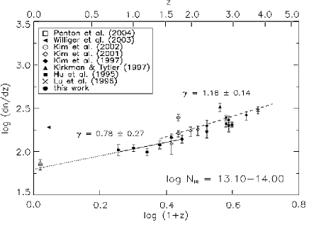
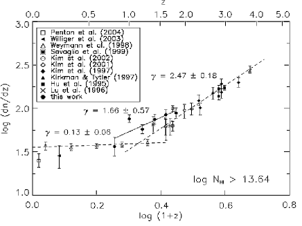
For , however, the number density evolves considerably faster than the constant comoving rate Tytler (1987b). Kim et al. (2002a) obtain for systems with column densities in the range . This corresponds to considerable evolution in the product . A smooth transition is found over the redshift range by Janknecht et al. (2006), with a dependence of the evolution rate on column density. High column density systems corresponding to Lyman Limit Systems evolve somewhat more slowly than lower column density systems. Stengler-Larrea et al. (1995) find for systems with , over the redshift range . Based on a larger, higher redshift sample, Péroux et al. (2003) find somewhat more rapid evolution, with over the redshift range . Damped LyAbsorbers show evolution comparable to that of the Lyman Limit Systems, with increasing by about a factor of 2 from to Prochaska et al. (2005).
As will be discussed in § VI below, numerical simulations show that the structure of the IGM evolves, although in the comoving frame the structure is remarkably stable. Because is fit for a fixed H column density range, the diminishing gas density towards decreasing redshifts will result in fewer systems satisfying the column density threshold, so that will decrease towards decreasing redshift. Evolution in the ionizing background will also affect the number of absorption systems lying above the column density threshold, and this is a major factor in the evolution of . The slowdown at in the evolution is in fact attributed predominantly to a reduction in the intensity of the ionizing background: as the ionizing rate decreases, fewer systems will slip below the column density threshold than under pure density evolution. As a result, the decrease in towards lower slows down. The difference in the rate of evolution between low column density and high column density systems found by Janknecht et al. (2006) (compare Figs. 6 and 7), shows that structural evolution in the IGM must also play a role.
II.2.3 Characteristic sizes and spatial correlations
Multiple QSOs in proximity to each other on the sky provide an invaluable means for estimating the physical sizes of the regions in the IGM that give rise to the absorption features. Especially useful have been multiply imaged lensed quasars. Using high resolution spectra of a pair of images of a lensed QSO with a separation of 3 arcsecs, Smette et al. (1995) detected a large number of absorbers coincident between the two lines of sight. All the clearly detected coincident systems show comparable equivalent widths between the lines of sight, suggesting the same physical structures are being probed. These authors set lower limits of about 70 kpc for weak absorption systems (), and of about 15 kpc for strong systems (), assuming the clouds are spherical. For disk-like systems, the lower limits are about twice as large.
Other efforts resulted in similar lower limits McGill (1990); Bechtold et al. (1994); Smette et al. (1992). Multiple lines of sight with wider separations of about 1 arcminute suggest still larger sizes of 0.3–1 Mpc Dinshaw et al. (1998); D’Odorico et al. (1998b); Petitjean et al. (1998); Crotts and Fang (1998), and possibly as large as 40 Mpc (comoving) Williger et al. (2000). Smette et al. (1995) report a likely size of about 10–30 kpc for a single Damped LyAbsorber, comparable to the lower limit obtained by direct H imaging measurements of a separate system by Briggs et al. (1989).
A difficulty with interpreting the larger Megaparsec-scale sizes for the Lyforest systems is that the equivalent widths of systems with common redshifts along the neighboring lines of sight do not always match well over these scales. An alternative interpretation of the coinciding redshifts is that they indicate underlying spatial correlations between the absorption systems rather than their spatial coherence. Measurements of the auto-correlation function between absorption systems along single lines of sight suggest correlations on scales of a few hundred scales Meiksin and Bouchet (1995); Cristiani et al. (1995); Hu et al. (1995). An anti-correlation at separations of Meiksin and Bouchet (1995); Cristiani et al. (1995); Hu et al. (1995) has been disputed by Kim et al. (1997) on the basis of the limited lines of sight analysed, but the issue appears not fully resolved. In the presence of correlations, the error on the correlation function depends on the 3 and 4-pt functions, which are not well-measured. A more recent analysis at detects only weak positive correlations on the few hundred scale, and no clear anti-correlation Janknecht et al. (2006). Transverse positive spatial correlations over comparable scales at were obtained by Crotts and Fang (1998) and at by Petry et al. (2006). Coherence in absorption lines along lines of sight separated by Mpc at has been detected by Casey et al. (2008).
A characteristic size of 70 kpc for systems with suggests a large fraction of the baryons are contained within the Lyforest Meiksin and Madau (1993). Taking the size to correspond to a characteristic line-of-sight thickness, the corresponding H number density is . Ionization equilibrium in a UV background producing an ionization rate of H atoms per second (§ IV.1.2 below), gives a neutral fraction of , where is the radiative recombination rate for gas at a temperature K and . The ratio of the baryonic mass density of the Lyforest to the critical Einstein-deSitter density is
| (28) | |||||
for with and , and with and , evaluated at with and . This is comparable to estimates for the baryon density of the Universe (see § II.2.4 below). The result is not conclusive, however. Since the size estimates are in the transverse direction, a much smaller value for is possible if the structures are flattened, down by the aspect ratio of the thickness to breadth of the systems Rauch and Haehnelt (1995).
II.2.4 Deuterium absorption systems
High column density Lyabsorption systems offer the opportunity to measure the primordial deuterium abundance , a sensitive indicator of the cosmic baryon density, or equivalently the nucleon to photon ratio , according to Big Bang nucleosynthesis. To date, a relatively limited number of accurate determinations of from the deuterium abundance have been possible. A line of sight must meet several criteria to be useful for obtaining a clean measurement Kirkman et al. (2003): the hydrogen column density must be sufficiently large that deuterium is detectable; the velocity width of the system must be sufficiently narrow so as not to encroach on the offset deuterium feature; the structure of the system must not be so complicated that a weak interloping H feature could be mistaken for deuterium; and the background QSO must be sufficiently bright to obtain a high signal-to-noise ratio measurement. These combined criteria whittle down the number of acceptable QSO lines-of-sight to about 1% of those available at .
Despite the difficulty, several accurate determinations have been made Burles and Tytler (1998a, b); O’Meara et al. (2001); Pettini and Bowen (2001); Kirkman et al. (2003); Levshakov et al. (2002); Crighton et al. (2004); O’Meara et al. (2006). The current best estimate for is O’Meara et al. (2006). Using standard Big Bang nucleosynthesis models, this translates to a baryon density parameter of , where the errors refer to the error on the measurement and the uncertainties in the nuclear reaction rates, respectively. This corresponds to a nucleon to photon ratio of . This compares favorably to the determination from the 5-year WMAP measurements of the CMB fluctuations, combined with Baryonic Acoustic Oscillations and Type Ia supernovae constraints, of Komatsu et al. (2008).
II.2.5 Helium absorption systems
The UV spectral capability of the Hubble Space Telescope made it possible for the first time to measure intergalactic He Ly. Using the spectrum of Q0302003 at observed by the Faint Object Camera, Jakobsen et al. (1994) found (90% confidence) at , revised to a 95% confidence interval of by Hogan et al. (1997) and to by Heap et al. (2000) after more detailed modeling of the absorption trough. Because the same sources which ionize the H should also ionize He , virtually all the intergalactic helium will be in the form of either He or He , depending on whether or not there were sources hard enough to fully ionize helium.
Remarkably, using the spectrum of HS 17006416 () observed by the Hopkins Ultraviolet Telescope (HUT), Davidsen et al. (1996) measured the more moderate optical depth of over the somewhat lower redshift range . This led to the speculation that He was ionized around . Subsequent measurements of the spectrum of HE 23474342 () have shown the He Lyoptical depth to be very patchy at , as if a second reionization epoch were being observed, that of He Reimers et al. (1997).
Observations of PKS 1935692 () using HST Anderson et al. (1999) and of HE 23474342 using the Far Ultraviolet Spectroscopic Explorer have detected a He Lyforest Kriss et al. (2001); Zheng et al. (2004b); Shull et al. (2004), permitting more detailed assessments of the fluctuations in the He to H column densities. Measurements of the He Lyforest also provide an opportunity to probe the underlying IGM velocity field. Using combined FUSE and VLT data, Zheng et al. (2004b) were able to identify isolated absorption systems in underdense regions with common H Lyand He Lyfeatures. A comparison between the fit Doppler parameters gives the ratio . According to Eq. (11), this indicates a velocity field in underdense regions with kinematic motions that dominate the thermal.
Subsequent measurements continue to confirm the patchy nature of the He Lyoptical depth, including HST observations of HE 23474342 Smette et al. (2002), SDSS J23460016 () Zheng et al. (2004a), and Q11573143 ()Reimers et al. (2005), and a FUSE observation of HS 17006416 Fechner et al. (2006). As some of these references point out, and as will be discussed in § IV.3.2 below, the interpretation in terms of reionization is not unambiguous: the patchiness may also arise from fluctuations in the radiation field.
II.2.6 Metal absorption systems
The earliest identifications of intervening absorption systems were for elements heavier than helium, so called metals Bahcall et al. (1968). Common are carbon, nitrogen, silicon and iron, but to date the list extends much further, including oxygen, magnesium, neon, and sulfur Sargent et al. (1980); Meyer and York (1987); Cowie et al. (1995); Koehler et al. (1996); Songaila and Cowie (1996); Lu et al. (1998a); Ellison et al. (1999a, b); Schaye et al. (2000a); Simcoe et al. (2002, 2004); Richter et al. (2004); Savage et al. (2005). The metals provide invaluable insight into the structure of the IGM in several different ways. The widths of metal absorption features allow direct estimates of the temperature of the IGM and its small-scale velocity structure. The narrow widths of C features were used by York et al. (1984) to demonstrate the absorbers had the characteristic temperatures of photoionized gas rather than collisionally ionized. The metal systems probe the impact star formation has had on the IGM, as the metals were most likely transported into the IGM through galactic winds, or introduced in situ by local small-scale regions forming first generation, Population III, stars. In the nearby Universe, they indicate the presence of shocked gas, as may accompany the formation of galaxy clusters. As such, the metals in principle document the history of cosmic structure and star formation. Ratios of the metal column densities may be used to constrain the spectral shape of the metagalactic ionizing UV background, which in turn puts constraints on the possible sources of the background and their relative contributions. Lastly, metal absorption lines offer a unique opportunity to search for variability in the constants of nature.
Tables of the resonance lines most easily detectable in intervening absorption systems are provided by Morton and York (1989) and Vogel and Reimers (1995). Searches for intervening metal absorbers have been facilitated by the exploitation of atomic line doublets for some of the stronger species. The most common doublets used are Mg Å and C Å. These are among the strongest lines detected in the Lyforest. They also have the important advantage of wavelengths redward of Ly, placing them outside the Lyforest and avoiding this potential source of confusion. Searches for Mg absorption systems are by far the most common because of their established connection to galaxies. Mg absorber surveys were carried out by Lanzetta et al. (1987), Tytler et al. (1987), Sargent et al. (1988b), Steidel and Sargent (1992), Boisse et al. (1992), Aldcroft et al. (1993), Le Brun et al. (1993), Churchill et al. (1999), Nestor et al. (2005), York et al. (2006), Lynch et al. (2006), Nestor et al. (2006), Fox et al. (2006) and Narayanan et al. (2007). Surveys of C absorption systems were conducted by Sargent et al. (1988a) and Misawa et al. (2002). Absorption features by O Å are more difficult to identify since they lie within the Lyforest, and so are not easily distinguished from the forest. Searches have been successful, however, and have moreover discovered a second IGM environment. While at high redshifts the O systems probe the component of the IGM containing C Burles and Tytler (1996, 2002); Kirkman and Tytler (1997b), at low redshifts they are associated with a warm-hot intergalactic medium (WHIM) Tripp and Savage (2000); Savage et al. (2002); Richter et al. (2004); Danforth and Shull (2005, 2008); Tripp et al. (2008), that is most likely collisionally ionized rather than photoionized. A search for O absorption systems as an indicator of a WHIM at high redshift was conducted by Simcoe et al. (2002). Efforts are currently underway to detect an intergalactic x-ray absorption line forest using the XMM-Newton and Chandra x-ray satellites Nicastro et al. (2005); Kaastra et al. (2006); Rasmussen et al. (2007). Detections of low redshift O have been reported by Fang et al. (2002, 2007) and Williams et al. (2007).
Attempts to infer the origin of the metals, whether distributed by galactic outflows or introduced locally by Population III stars, have led to various efforts to estimate the range in ambient metallicities and to determine their spatial distribution Bergeron and Stasinska (1986); Bergeron et al. (1994); Cowie et al. (1995); Songaila and Cowie (1996); Cowie and Songaila (1998); Barlow and Tytler (1998); Ellison et al. (2000); Songaila (2001); Aracil et al. (2004); Songaila (2005, 2006); Pieri et al. (2006); Simcoe et al. (2006); Scannapieco et al. (2006b). Updated solar abundances useful for modeling the abundances of the metal absorption systems are provided by Grevesse and Sauval (1998), Holweger (2001), Allende Prieto et al. (2001, 2002) and Asplund (2003). Early attempts to tease out weak metal features were based either on a spectral shift-and-stack approach to generate a high signal-to-noise ratio composite C line Lu et al. (1998b) or through a pixel-by-pixel statistical analysis of the spectra Songaila and Cowie (1996); Cowie and Songaila (1998). A comparison of these two techniques is provided by Ellison et al. (2000).
An alternative is to perform long integrations of bright QSOs to obtain high resolution, high signal-to-noise ratio spectra. With signal-to-noise ratios of 200–300 per spectral resolution element, Simcoe et al. (2004) detected metal lines in 70% of the Lyforest systems. Absorption systems with H column densities as low as show C features, while systems with show O features. Although the inferred metallicities are model dependent (fixed in part by the assumed spectrum and intensity of the ionizing background), the measurements suggest metallicities as low as that of the Sun. No evidence for a metallicity floor could be discovered. The metallicity distribution inferred is consistent with a lognormal distribution with a mean of 0.006 solar.
The mechanism and degree of metal mixing in the diffuse IGM are unclear. While the mixing of metals in stellar interiors by convection and diffusion may produce a homogeneous composition, preserved in supervovae ejecta and winds, it is far from clear that the mixing of the ejecta will result in uniform metallicity. The mixing process is still poorly understood in the Interstellar Medium, and much more so in the IGM. Just as stirring a drop of milk in a cup of coffee will result in the mixing and intermingling of the two fluids, so may the stirring produced by dynamical instabilities such as the Kelvin-Helmholtz and Rayleigh-Taylor mix metal enriched stellar ejecta with the surrounding primordial gas. Insufficient mixing, however, rather than a uniform mixture, will instead result in striations or patches of high metallicity gas entrained within the primordial gas of essentially zero metallicity. Schaye et al. (2007) find evidence for just such inadequate mixing for diffuse absorption systems (with a median upper limit of 13.3 on ), at . By combining C measurements with upper limits on H , C , Si , Si , N and O , they place robust constraints on the metallicities and physical properties of the C absorption systems, with a median lower limit on the metallicities of and a median upper limit on the absorber sizes of kpc. They obtain typical median lower and upper limits on the hydrogen densities of and , a range that suggests a cloud size of about 100 pc. The clouds, however, would likely be transient, either quickly dispersing if freely expanding or shorn apart by dynamical instabilities if moving relative to a confining medium, on a timescale of about yrs. Schaye et al. (2007) arrive at a picture in which new clouds are continuously created through dynamical or thermal instabilities. In this picture, nearly all the metals in the IGM could be processed through just such a cloud phase. The dispersed clouds would retain their coherence as small patches, but of too low column density to be detectable. The resulting IGM metallicity would persist as patchy, not mixed.
Matching the metal absorption lines to the corresponding H Lyfeatures frequently reveals multicomponent substructure obscured by the width of the Lyfeature. An example from QSO is shown in Fig. 8. The C systems show evidence for spatial clustering on scales of up to Rauch et al. (1996); Songaila and Cowie (1996); D’Odorico et al. (1998a); Pichon et al. (2003). This is consistent with a lower limit of kpc for the clustering of C and Mg systems obtained by Smette et al. (1995) based on a statistical analysis of coincident metal systems in neighboring lines of sight to a lensed QSO. An analysis of a triply imaged quasar at by Ellison et al. (2004) shows that high ionization systems like C and Si absorbers retain coherence over scales of kpc. By contrast, low ionization systems like Mg and Fe absorbers show coherence only over much smaller scales. Assuming a spherical geometry, they are estimated to have sizes of 1.5–4.4 kpc (95% c.i.). Using similar measurements, Rauch et al. (2001) find C systems at are coherent over scales of about 300 pc, with column densities along neighboring lines of sight differing by 50% for separations of about 1 kpc. Detectable levels of C extend over scales of several kiloparsecs.
Damped LyAbsorbers show a wide range of metals with both low and high ionization states, including boron, carbon, nitrogen, oxygen, magnesium, aluminum, silicon, phosphorus, sulfur, chlorine, argon, titanium, chromium, manganese, iron, cobalt, nickel, copper, zinc, germanium, arsenic and krypton Lu et al. (1996a); Wolfe et al. (2005); Dessauges-Zavadsky et al. (2006). The metallicities evolve from about 0.03 solar at to 0.15 solar at , with few above 0.3 solar Wolfe et al. (2005). No DLA is found with a metallicity smaller than 0.0025 solar, distinguishing them as a population from the Lyforest. By contrast, super Lyman Limit Systems are found to have metallicities ranging from 0.1 solar to super-solar abundances with as much as 5 times solar in zinc Kulkarni et al. (2007). As both these classes of systems are likely related to galaxies, further discussion of them is deferred to § VIII.
The presence of the metal lines in absorbers of all H column densities in principle offers an opportunity to obtain a nearly model-free measurement of the gas temperature. Allowing for kinetic broadening of the Doppler parameters following Eq. (11), the measurements of the Doppler parameters from features corresponding to two or more elements permits the thermal and kinematic broadening components to be separated. (In principle, instrumental broadening could be incorporated into the kinematic term.) Given total Doppler parameter measurements and for two species and of masses and , the temperature may be solved for as
| (29) |
Applying this method to C and Si features detected in three high redshift QSOs, and assuming that the C and Si features trace the same systems with the same temperature and velocity structure, Rauch et al. (1996) obtain a typical temperature of K and typical kinetic motions of for a select subsample of especially well-fit features. The large C column densities of the systems (typically exceeding , M. Rauch, personal communication), suggest large H column densities of Simcoe et al. (2004).
A few other Lysystems selected for quiescent velocity fields as part of a program of deuterium abundance measurements yield somewhat cooler temperatures. The Doppler parameters of C and Si measured by Kirkman et al. (2000) in a system with yields a temperature of K. For a Lyman Limit System with at Tytler et al. (1999), the Doppler parameter measured for Mg compared with that of H gives K and , assuming the hydrogen and metals sample the same velocity field, which is not an obvious assumption to make. For a super Lyman Limit System with , O’Meara et al. (2001) find from a simultaneous fit to O , N and H K and . In all cases, the temperatures obtained are consistent with photoionization heated gas. Although direct gas density measurements are not possible, models generally suggest that higher column density systems correspond to higher densities, especially at these high values. The temperatures support the expected trend of decreasing temperature with increasing density for sufficiently dense absorption systems Meiksin (1994).
The small kinetic contributions to the line broadening are in contrast to what is found for He absorption systems, which appear to be dominated by kinetic broadening Zheng et al. (2004b). The He features, however, were chosen for their clear isolation in the spectrum, and so may probe physically underdense regions, in contrast to the higher column density systems above. An attempt to estimate temperatures from a larger sample of He and H systems has not been able to produce secure values, but nonetheless shows that only of the lines are dominated by kinematic broadening Fechner and Reimers (2007).
Intergalactic metal absorption systems may be used to probe the time variability of fundamental physical quantities over cosmological timescales. The excitation of ionic fine-structure levels by the CMB allows metal lines in the Lyforest to be exploited for measuring the evolution of the CMB temperature Bahcall and Wolf (1968). Because of the possible influence of other excitation mechanisms, the measurements are strictly speaking upper limits. Existing excitation temperature measurements are K at Songaila et al. (1994), K at Ge et al. (1997), K at Ge et al. (2001), and K (95% c.i.) at Molaro et al. (2002). These values are all consistent with a linearly evolving CMB temperature of , expected for a homogeneous and isotropic expanding universe, with K Mather et al. (1999).
Detected resonance line multiplets have been used to place constraints on the time variation of fundamental constants. Bahcall et al. (1967) used the fine structure wavelength splittings of the Si lines near Å and Å and the Si lines near Å to show that the fine structure constant () varies by less than 5% between and . Tentative evidence for an evolving fine structure constant between of was reported by Webb et al. (1999) using measurements of Mg and Fe transitions. The value was later revised to over the redshift range Murphy et al. (2004), suggestive of a positive detection of a variation. There is by no means concensus on the detection. Chand et al. (2004) and Srianand et al. (2004) report over the redshift range . Their analysis method has been contested by Murphy et al. (2007) and Murphy et al. (2008), and defended by Srianand et al. (2007). In an independent effort using a modified technique designed to eliminate some systematics, Levshakov et al. (2007) obtain between and . Including the hyperfine splitting of the hydrogen 21cm line permits constraints on the variation of , where is the electron to proton mass ratio and is the proton gyromagnetic ratio. The current best limits are, for a linear fit over the redshift range , Tzanavaris et al. (2005). Combining H 21cm data and OH 18cm data, Kanekar et al. (2005) obtain a limit on the effective combination of between and .
II.3 Direct flux statistics
While the absorption line parameters relate most directly to the physical characteristics of the absorption systems, measuring similar parameters in numerical simulations can be very computationally demanding, particularly when building up sufficient statistics to make such a comparison meaningful. More straightforward comparisons may be made using the flux statistics directly. The statistical measures in most use are the mean transmitted flux, the transmitted flux per pixel probability distribution, the flux power spectrum and its Fourier transform, the flux autocorrelation function. An additional analysis based on wavelets permits a quick means of gauging the distribution of widths of the absorption features.
II.3.1 Mean transmitted flux
By far the simplest statistic is the mean transmitted flux through the IGM. Oke and Korycansky (1982) introduced two measurements, , the mean flux of a background source removed by scattering between the Lyand Lytransitions in the restframe of the QSO (but avoiding emission line wings), and , the mean flux removed between Lyand the Lyman edge. These definitions are straightforwardly generalized to the fraction of flux removed between each successive pair of Lyman transitions. Removing the effect on higher orders by lower orders, however, is not straightforward but may be accomplished in a statistical sense Press et al. (1993). The measurement may be evaluated as , where is the measured flux in pixel , is the corresponding predicted continuum of the background object, normally a QSO, and the average is carried out over a given wavelength (or corresponding redshift) interval between Lyand Lyin the restframe of the QSO. Considerable care must be taken in measuring the contribution at a given redshift from Lyalone. Systematics that would bias the result if not corrected for include: 1. a low H fraction near the QSO due to its own ionizing intensity (the “proximity effect”), 2. contamination by metal absorption systems, 3. the large stochastic influence of Lyman Limit Systems and Damped LyAbsorbers, the latter of which produce a divergent mean Meiksin and White (2004), and 4. evolution of the absorption in the region measured, including over individual pixels of the spectrum. A detailed discussion is provided by Tytler et al. (2004a).
For a spectrum that may be decomposed into individual absorption features with equivalent widths depending on some set of parameters , such as column density or Doppler parameter, the mean of the transmitted flux is given by
| (30) |
with the effective optical depth due to the lines given by
| (31) | |||||
where is the number of systems per unit rest wavelength per unit volume in parameter space Spitzer (1948); Press et al. (1993), here represented in terms of the number per (proper) equivalent width per unit redshift . The variance of the transmission depends on the details of the line profiles. Expressions for idealized examples are provided by Münch (1968) and Press et al. (1993).
It is instructive to consider a comparison between Eq. (31) and the Gunn-Peterson optical depth (15). Using Eq. (27) for the number density evolution given by and Eq. (24) for systems on the linear part of the curve-of-growth, may be recast in the form of the Gunn-Peterson optical depth
| (32) |
for a mean distributed scattering gas density , where is the mean column density of the absorption systems with mean atomic density and line of sight thickness , and is the porosity of the absorbers, equivalent to the spatial filling factor of the absorption systems for . For a column density distribution varying like , the effective absorber optical depth (excluding DLAs) is dominated by saturated systems, with . In this case, Eq. (21) gives . If the absorber velocity widths scale like the Hubble expansion across them, , Eq. (31) gives instead of Eq. (32),
| (33) |
In practice the effective optical depth will scale somewhat between the linear and saturated line limits. It will not in general scale like the Gunn-Peterson optical depth Eq. (15), as is often asserted in the literature. For , Eq. (31) instead gives the dependence . This is corroborated by estimates of the mean H transmission due to Lyscattering from all components, whether or not they may be modeled as individual Voigt profile absorption systems. More generally, the mean transmission may be expressed as
| (34) |
From an analysis of Lyscattering by the IGM in the redshift range using moderate resolution spectra, Press et al. (1993) obtained with and . The evolution exponent agrees closely with the finding of Kim et al. (2002a) for above. A similar result was obtained by Kim et al. (2001) using high resolution spectra: and (as inferred by Meiksin and White (2004)). Kim et al. (2002a) give the slight variation based on an expanded data set of and . Because the implied probability distribution for is skewed, the statistical expectation value for the mean transmission must be computed from these expressions for using Monte Carlo integration Meiksin and White (2004). A good fit to the evolution of based on the data compiled by Meiksin and White (2004), extended to lower redshifts using the data of Kirkman et al. (2007), is given by
Meiksin (2006a). The evolution is found to vary from relatively slowly at low redshifts, as expected for discrete saturated features, to the more rapid evolution of the Gunn-Peterson effect at high redshifts as the porosity of the absorption systems approaches unity and increasingly diffuse gas dominates the effective optical depth.
A dip in the evolution of at was reported by Bernardi et al. (2003) based on a sample of 1061 moderate-resolution QSO spectra measured by the SDSS. The feature was interpreted as evidence for sudden heating due to the onset of He reionization. This interpretation is not supported by recent simulations McQuinn et al. (2008). The feature was not confirmed by McDonald et al. (2006) using an alternative analysis method applied to 3035 SDSS QSO spectra. Using a sample of 86 high-resolution high signal-to-noise ratio spectra, however, Faucher-Giguère et al. (2008b) find a feature similar to that reported by Bernardi et al. (2003). The existence of the feature appears still not to be entirely secure, but tentatively suggests that a physical change in the state of the IGM occurred at , possibly reflecting a change in the H ionization rate, perhaps owing to the growing influence of QSOs (§ IV.1.2).
II.3.2 Statistics based on pixel fluxes
More detailed transmission information may be extracted from the use of the full spectrum, including the probability distribution of the transmission per pixel, the flux power spectrum, the autocorrelation function of the transmission, and a wavelet decomposition. Because these statistical measures are best interpreted in conjunction with numerical simulations, they are discussed in more detail in § VI. Here they are only defined.
The pixel transmission distribution (PTD) and its variants, like the transmission flux probability distribution function (TFPDF) McDonald et al. (2000), simply quantify the frequency of occurrence of a given flux value in each pixel of the spectrum, normalized by the continuum, often expressed in frequency bins. It was introduced by Jenkins and Ostriker (1991) to search for underlying intergalactic absorption in excess of the amount accounted for by discrete absorption systems. Several tabulations are available in the literature: Rauch et al. (1997b), McDonald et al. (2000), Becker et al. (2007), Desjacques et al. (2007) and Kirkman et al. (2007).
Second order statistics include the flux autocorrelation function and the flux power spectrum, in analogy to similar statistical descriptions of the clustering of galaxies. The flux transmission autocorrelation function was introduced by Zuo and Bond (1994) to investigate properties of the Lyforest. For a velocity separation , it is defined by
| (36) |
where denotes the pixel flux at velocity , and is the measured mean flux at the relevant redshift.151515This differs somewhat from the definition of Zuo and Bond (1994), who in place of in the denominator, used the more general form . In most of the literature, it is assumed the mean flux changes negligibly over the velocity separations for which it is computed. This will break down for sufficiently large velocity separations that cosmological expansion becomes a factor, but in this case the physical interpretation of the autocorrelation function becomes less transparent as it would correlate transmissions at different cosmological epochs. Several estimates of are provided in the literature: Zuo and Bond (1994), Liske et al. (2000), McDonald et al. (2000), Croft et al. (2002b), Becker et al. (2004), D’Odorico et al. (2006), McDonald et al. (2006) and Kirkman et al. (2007). The results generally show significant correlations over scales of a few Megaparsecs (comoving). Similar to the flux autocorrelation function is the flux cross-correlation function along neighboring lines of sight to QSOs near each other on the sky Liske et al. (2000); Becker et al. (2004); D’Odorico et al. (2006). Cross-correlations of similar strength to the autocorrelations are found, extending over similar spatial scales.
The flux power spectrum has received considerable attention as a means of constraining cosmological parameters Croft et al. (1998); Hui et al. (2001). It is a measure of the variance in the amplitude of the Fourier transform coefficients of the transmitted flux. Defining and its Fourier transform
| (37) |
over the velocity interval , the flux power spectrum is
| (38) |
The dimensionless form is often more convenient. It forms a Fourier transform pair with the flux autocorrelation function through
| (39) |
The reader should be aware that several different conventions for exist in the literature, some without a mean flux normalization, some differing by a factor of , and some referring to an effective 3D flux power spectrum extracted from the 1D flux power spectrum in a manner analogous to the relation between the 1D and 3D mass power spectra. Many tabulations of are available: Croft et al. (1998), Croft et al. (1999), McDonald et al. (2000), Croft et al. (2002b) and Kim et al. (2004b, a). A substantial effort was made to measure from the spectra of high redshift quasars discovered by the Sloan Digital Sky Survey McDonald et al. (2006).
A shortcoming of the Fourier transform is that it loses spatial information. In the case of a spectrum showing the Lyforest, the positions of individual absorption features are lost. A wavelet transform is analogous to a Fourier transform, but retains local information, giving in effect a description of the power on different scales as a function of position. A wavelet is a square-integrable function, , defined in real space such that (where and are integers) forms an orthonormal basis for the set of square-integrable functions. It satisfies , and is normally concentrated near . The wavelet coefficients are defined by ; the original function may be recovered through . The wavelet transform effects a localized multiscale rendition of the data. Although not commonly used, wavelets are in principle a powerful tool for analysing the Lyforest, producing a statistical description similar to the distribution of -values. The discrete wavelet transform, like the fast Fourier transform, may be computed extremely rapidly, permitting a large number of spectra to be analyzed much more quickly than by performing a full absorption line analysis. This is an advantage over full Voigt profile line fitting for assessing the match of simulations to observations Meiksin (2000); Theuns and Zaroubi (2000); Meiksin and White (2001); Meiksin et al. (2001); Theuns et al. (2002a); Zaldarriaga (2002).
III Ionization Equilibrium
III.1 Ionization
III.1.1 Hydrogen and helium
The absorption signatures of the IGM are produced by atoms and ions with bound electrons, either through resonance scattering or photoelectric absorption. The amount of scattering or absorption depends on the ionization structure of the IGM. In this section, the photoionization of hydrogen and helium is discussed. In hot environments like galaxy clusters, collisional ionization can dominate. Collisional ionization equilibrium may play a particularly important role in the physics of the WHIM Cen and Ostriker (1999); Davé et al. (1999, 2001); Cen and Ostriker (2006) and is treated more generally in the section below on metal ionization.
Photons with energies exceeding the ionization potential of a bound electron in a hydrogen atom will ionize the neutral hydrogen atoms in the IGM at the rate per neutral atom
| (40) |
where is the hydrogen photoelectric cross section, is the threshold frequency required to ionize hydrogen (the Lyman limit), and is the specific energy density of the ambient radiation field. The specific energy density is related to the specific intensity of the radiation field by , where is the angle-averaged specific intensity.
Free electrons will be radiatively captured by the protons at the rate per proton , where , often referred to as the Case A radiative recombination coefficent , is the total rate coefficient for radiative capture summed over recombinations to all energy levels. Expressed in terms of the ionization fractions and , where is the total hydrogen number density, the ionization rate equations become
| (41) |
The time-derivatives are lagrangian, so that Eqs. (41) are valid in the presence of velocity flows.
In equilibrium, the neutral fraction will be
| (42) |
For a pure hydrogen gas, , and the rate equation for becomes
| (43) |
where is the total radiative recombination time for the gas. The equilibrium neutral fraction may be expressed as
| (44) |
where denotes the number of photoionizations per neutral atom over a recombination time. It is instructive to consider the case of constant . Eq. (43) then has the general solution
| (45) |
where , , and is the initial deviation of the neutral hydrogen fraction from its equilibrium value. For a fast photoionization rate (), and . An initial deviation from equilibrium decays exponentially. The neutral fraction approaches its equilibrium value on the photoionization rate timescale , regardless of whether equilibrium is established through net photoionizations or net recombinations. Ionization equilibrium will be maintained provided any change to the gas (such as source variability or the expansion of the gas) occurs on a time scale long compared with the photoionization time scale. By contrast, for a slow photoionization rate , and the neutral fraction approaches equilibrium on the recombination timescale, for ().
The photoionization equations for helium are analogous to Eqs. (41). Denoting the respective He , He , and He fractions by , and , they are given by
| (46) |
where and are the total recombination rates to all levels of He and He , respectively, and and are the respective photoionization rates. The total electron density is .
The Case A radiative recombination coefficient for hydrogenic ions is provided by Seaton (1959), from which the coefficients for and may be derived. (In general, the radiative recombination coefficient for a hydrogenic ion of atomic number is related to that of hydrogen by .) For elements He and beyond, the recombination coefficient is the sum of two rates. One is the usual radiative capture term, in which for a species with electrons. The other arises from dielectronic recombination, in which a fast incoming electron excites an ion, which becomes trapped in a weakly bound autoionizing state upon capturing the electron, then decays by the emission of a resonance line photon: . The probability for emission of the photon is suppressed by the factor ; usually excitation is followed by the reverse reaction. A form for the radiative recombination rate coefficient contribution to for He He is provided by Verner and Ferland (1996), while a form for the dielectronic term is provided by Aldrovandi and Pequignot (1973). The recombination coefficients are listed in Table LABEL:table.RecombCoef. Recombination to He may also occur through charge transfer, , where is the energy defect. Where hydrogen is highly ionized, this is a negligible effect compared with radiative recombinations. For partially ionized hydrogen, however, as for example within a Damped LyAbsorber, or the IGM prior to its complete reionization, the effect may play an important role. The rate coefficient is provided by Kingdon and Ferland (1996). The reverse process, charge transfer ionization, is suppressed by a Boltzmann factor and so is normally negligible except at high temperatures.
| [Hz] | ||||
|---|---|---|---|---|
| 1.34 | 2.99 | |||
| 1.66 | 2.05 | |||
| 1.34 | 2.99 |
The exact photoionization cross section for hydrogenic atoms with atomic number in the ground state is Heitler (1954)
| (47) |
for eV, the threshold energy for ionization, and where , where is the Bohr radius, is the fine structure constant, and . For most practical applications, however, an approximate form is preferred. The ionization cross sections are well-approximated by the form given by Osterbrock (1989),
| (48) |
The parameters for hydrogen and helium are listed in Table LABEL:table.CrossSection. For results requiring very high accuracy, more precise fits to the photoionization cross sections are provided by Verner et al. (1996), including results for an exhaustive list of metals.
III.1.2 Metals
The large number of ionization states of metals results in more complex processes involved in their photoionization. These include autoionization and Auger electron production in addition to dielectronic recombination. In an autoionization, an excited ion with one or two electrons lying in the photoionization continuum is produced following a photoionization event in which a deep shell electron is ejected. The excited ion spontaneously ionizes through a radiationless transition and the ejection of multiple Auger electrons. Although there has been considerable progress in accurate estimates of all the relevant rate coefficients, many remain poorly determined either experimentally or theoretically, requiring interpolation (and sometimes extrapolation) from coefficients known for related species Ferland and Savin (2001). These uncertainties can affect the predicted metal abundances in the absorption systems. The effect of uncertainty in the dielectronic recombination rates on commonly measured metal features is discussed by Savin (2000). Some of the methods of approximation are described in the literature for the rate coefficients (see below).
Sophisticated computer codes have been developed to solve for the equilibrium ionization states. A widely used publicly-distributed code is CLOUDY Ferland et al. (1998), which solves the radiative transfer problem for plane-parallel and spherical geometries. The photoionization of intervening absorption systems has been described by Verner and Iakovlev (1990), whose formulation is followed here.
Denote by the fraction of a particular element in the ionization state, so that runs from 1 (neutral) to (fully ionized) for an element of atomic number . Then . The general rate equation for is
| (49) | |||||
where is the collisional ionization rate Voronov (1997), the autoionization rate Arnaud and Rothenflug (1985), the photoionization rate without post-ionization Auger-electron ejection Verner et al. (1996); Verner and Yakovlev (1995), the radiative recombination rate Verner and Ferland (1996); Shull and van Steenberg (1982b, a); Aldrovandi and Pequignot (1973); Arnaud and Rothenflug (1985), the dielectronic recombination rate Nussbaumer and Storey (1983, 1986, 1987), the rate of charge transfer ionization with H Kingdon and Ferland (1996), the rate of charge transfer ionization with He Arnaud and Rothenflug (1985), the rate of charge transfer recombination with H Kingdon and Ferland (1996), and the rate of charge transfer recombination with He Arnaud and Rothenflug (1985). Photoionization from deep shells followed by Auger-electron ejection, resulting in a change from an initial ionization state to a final state , occurs at the rate Kaastra and Mewe (1993). The convention that corresponds to recombination to ionization state and corresponds to collisional ionization of state is used. Because of the low metallicity of the IGM, the electron density may normally be well-approximated by the electrons lost only by hydrogen and helium.
Using the above notation for the various species and taking for hydrogen and for helium, Eqs. (41) and (46) are modified, allowing for collisional ionization and the charge transfer reactions, to
| (50) | |||||
where the first sum of the double sums is over all elements except the excluded one indicated.
Noting that the photoionization rates are proportional to the energy density of the radiation field, it follows from the structure of Eqs. (49) and (50) that the equilibrium fractions are determined by the ratio for a given spectral shape of the radiation field with photon number density , and for a given set of elemental abundances. The ratio is know as the ionization parameter. Larger values for generally produce higher ionization stages in the metals, although these also depend on the spectral shape of the radiation field. Comparisons with measured ion column densities may then be used to constrain the natures of the radiation field and the absorption systems.
Fitting formulas to collisional ionization, radiative recombination and dielectronic recombination rate coefficients are provided by Shull and van Steenberg (1982a). Improved values for many of these rates have since then become available, and have been referenced above. Power law fits to collisional and radiative recombination rates involving hydrogen and helium are provided by Abel et al. (1997). Fitting formulas to more recent rates for the elements hydrogen through nickel are provided by Mazzotta et al. (1998), along with equilibrium ionization fractions for metals in a hot environment, for which collisional ionization will normally dominate photoionization. A comprehensive compilation of the literature is available at D. Verner’s Atomic Data for Astrophysics website, 161616http://www.pa.uky.edu/verner/atom.html as described in Ferland et al. (1998). Since then, improved estimates have been obtained for some rates, including laboratory measured values of dielectronic recombination rates (Savin et al. (2006) and references therein). A comprehensive review of the atomic physics relevant to x-ray lines, as will arise from a warm-hot IGM, is provided by Kallman and Palmeri (2007).
III.2 Thermal equilibrium
In the presence of heat transfer at the rate per particle, where and are the thermal gain and loss functions per volume and is the particle density, the second law of thermodynamics requires the entropy per particle to change at the rate
| (51) |
where is the temperature of the system. For an ideal gas, the entropy per particle is , where is the gas pressure, is the mass density, is the ratio of specific heats at constant pressure to constant volume ( for a monatomic gas), is Boltzmann’s constant, and is an arbitrary additive constant. For numerical computations, it is often useful to express the energy equation in its entropic form Eq. (51), but through the entropy parameter
| (52) |
It follows from Eq. (51) that
| (53) |
The gas temperature is related to by
| (54) |
where is the mean mass per particle.
Photoionization will provide heat through the excess energy absorbed by an electron above the threshold energy required to ionize a given atom. For a single species of density , the photoionization heating rate is
| (55) |
where is the ionization potential of species . The total heating rate from all species is
| (56) |
The contributions due to the photoionization of the metals is normally negligible because of their low abundances.
Cooling is provided by recombinations, collisional excitation of the excited levels in neutral hydrogen, and inverse Compton scattering off CMB photons. At high temperatures, free-free losses and collisionally excited line radiation from atoms and ions other than neutral hydrogen may become important contributions as well. As for heating, all species contribute to cooling, giving the total cooling rate
| (57) |
For a single species, recombinations radiate the electron energy as photons at the rate . Recombination cooling coefficients are provided by Seaton (1959) for recombinations to H and He . An expression for the radiative contribution to for recombinations to He is provided by Black (1981). The dielectronic contribution may be approximated as Gould and Thakur (1970) using the second part of the expression for in Table LABEL:table.RecombCoef, which expresses the dielectronic component. The total recombination cooling coefficients are provided in Table LABEL:table.RecombCoef.
The cooling rate due to the collisional excitation of H by electrons is given to an accuracy of 3% over the temperature range K by the expression Spitzer (1978):
| (58) |
For temperatures relevant to the IGM, cooling losses due to collisional ionization of hydrogen and collisional excitation and ionization losses from helium are negligible. Similarly, for the low metallicities encountered in the IGM, radiative losses from metals are normally negligible, although they may possibly be important in the WHIM.
Cooling is also produced by the Compton scattering of CMB photons off the electrons, which is especially important at high redshifts. The cooling rate is Weymann (1965)
| (59) |
where is the Thomson cross section, is the radiation density constant, is the electron mass, is the speed of light, and is the temperature of the cosmic microwave background.
In the WHIM, cooling by thermal bremsstrahlung radiation, or free-free emission, due to the acceleration of a charge in the Coulomb field of another charge may be significant. For an ion of number density and charge , the cooling rate is Rybicki and Lightman (1979)
| (60) |
where is a frequency average of the velocity-averaged Gaunt factor, and ranges between 1.1 and 1.5. Shapiro and Kang (1987) provide the fitting formula for K and for K. Cooling rates including collisionally excited metallic line losses and their individual emissivities are provided by Gaetz and Salpeter (1983) for solar abundances. Non-solar values may be interpolated with the zero-metallicity limit for which atomic cooling is determined only by the hydrogen and helium losses.
Photoelectric heating by x-rays is automatically included in Eq. (55). X-rays, however, may introduce two other sources of energy exchange: gains through Compton heating and losses through the effect of secondary electrons.
Sources of high energy radiation, such as a hard x-ray background, may inject additional energy into the IGM through Compton heating Arons and McCray (1969); Rees (1969); Rees and Setti (1970); Madau and Efstathiou (1999). For an IGM of electron density and temperature , an x-ray background with energy density will heat the gas through Compton scatterings at the rate
| (61) |
For photons with energies exceeding 100 keV, Compton scattering takes place in the relativistic regime, requiring the Klein-Nishina cross section instead of the Thomson. The heating rate then becomes Blumenthal (1974); Madau and Efstathiou (1999)
| (62) | |||||
where . The Compton heating rate should then be added to Eq. (56).
The secondary electrons ejected by x-rays have only a small effect on the temperature of highly ionized gas. In partially ionized gas, however, their contribution to the energy losses may become appreciable. They play a particularly important role in the cooling of gas ahead of ionization fronts during the Epoch of Reionization. Expressions for the energy of a primary electron deposited as heat, further ionizations, and collisional excitations, for both hydrogen and helium, in a partially ionized medium are provided by Shull and van Steenberg (1985).
IV The Metagalactic UV Background
IV.1 Mean energy density of the UV background
IV.1.1 Origin of the UV background
Since the ionization structure of the IGM is determined by the specific radiation energy density of the metagalactic ultraviolet photoionizing background, a complete understanding of the structure of the IGM requires an estimate for . In turn, measured properties of the IGM, like its optical depth to hydrogen and helium ionizing photons or the ratios of ionization fractions of metals, place constraints on the shape of the metagalactic UV background.
In a homogeneous and isotropic expanding universe, Eq. (5) gives for the integrated specific energy density produced by sources with a total proper emissivity
| (63) |
where is an effective optical depth due to absorption by the IGM and . For discrete absorption systems, Eq. (31) may be used, adapted to photoelectric absorption by choosing and taking , where . Then, on replacing by ,
| (64) |
where
| (65) |
The emissivity consists of two contributions, isolated radiation sources, such as galaxies and QSOs, and diffuse emission from the IGM itself. Survey estimates for the contributions from isolated sources are discussed below. There are four principal contributions to the diffuse emission capable of photoionizing the IGM Haardt and Madau (1996): 1. recombinations to the ground state of H and He , 2. He Lyrecombination radiation, 3. He two-photon continuum emission, and 4. He Balmer continuum emission. The specific recombination emissivity associated with each of these processes may be expressed generally in the form Haardt and Madau (1996)
| (66) |
where
| (67) | |||||
where refers to the photoionization threshold for ionizing the ground state of an ion of atomic number . The function expresses the escape rate of recombination photons produced by discrete absorption systems in terms of the product of the fraction of photons of energy absorbed by a given ion, the probability that a recombination will result in the particular radiative transition considered, and the probability that the emitted photon will escape the absorption system that produced it. These factors may be computed from detailed radiative transfer computations using a code like CLOUDY Haardt and Madau (1996).
The capture of electrons into the level of a hydrogenic ion results in the emission of a continuum photon distribution sharply peaked at the photoelectric edge. The rate of direct recombinations may be computed from the Milne relation between the free-bound recombination cross section for an electron moving at velocity and the bound-free photoionization cross-section Rybicki and Lightman (1979)
| (68) |
where is the statistical weight for the atom with electron in the bound state and is the statistical weight for the ion. The bound-free cross-section from state in a hydrogenic atom of atomic number may be expressed as
| (69) |
where is a Gaunt factor and is the fine-structure constant. The Gaunt factor for the ground state is
| (70) |
where (cf Eq. [47]). The photon released following recombination will have energy , where is the mass of an electron and is Planck’s constant. For a Maxwellian velocity distribution for the electrons, the free-bound emissivity due to recombinations to state in a hydrogenic ion of atomic number and number density is then
| (71) | |||||
Recombinations to He produce hydrogen-ionizing photons (). The recombinations generally occur to high energy levels, followed by a cascade of bound-bound transitions. Recombinations that populate the level of He result in a He Lyphoton of energy 40.8 eV, which photoionizes neutral hydrogen in the Lyforest systems. Recombinations that populate the level produce He two-photon emission with a total energy of 40.8 eV and a spectrum peaking at 20.4eV. Direct recombinations to and produce He Balmer continuum emission, for which the threshold photoionization energy is the same as the hydrogen Lyman limit.
IV.1.2 Sources
| 2.75 | ||||||
|---|---|---|---|---|---|---|
| 3.00 | ||||||
| 3.89 | ||||||
| 4.00 | ||||||
| 5.00 | ||||||
| 5.50 | ||||||
| 6.00 |
QSOs were early recognized as a prominent source of metagalactic ionizing photons Rees and Setti (1970); Arons and McCray (1970b, a). Since then, there have been numerous estimates of their contribution to the UV metagalactic background Sargent et al. (1979); Bechtold et al. (1987); Miralda-Escudé and Ostriker (1990); Madau (1992); Miralda-Escudé and Ostriker (1992); Meiksin and Madau (1993); Giroux and Shapiro (1996); Haardt and Madau (1996); Fardal et al. (1998); Shull et al. (1999); Haardt and Madau (2001); Schirber and Bullock (2003). The QSO luminosity function is conveniently parametrized by a double power-law form Boyle et al. (1988)
| (72) |
where describes the spatial density of QSOs at redshift in the absolute magnitude range to , is a spatial normalization factor (normally expressed in comoving units), and is a characteristic break magnitude. In a Pure Luminosity Evolution (PLE) model, is held fixed while is allowed to evolve. In a Pure Density Evolution (PDE) model, is held fixed while is allowed to evolve. Although PLE and PDE models well fit the data over limited redshift ranges, Fan et al. (2001b) show that the steepness of the bright end of the luminosity function has evolved between and . Estimates of the QSO luminosity function at are provided by Croom et al. (2004) based on the 2dF redshift survey, and by Richards et al. (2005), combining data sets from the 2dF and SDSS. Richards et al. (2006) use the SDSS to measure the bright end of the QSO luminosity function and its evolution over the redshift range .
A long-standing uncertainty affecting estimates of the QSO contribution to the UV background at high redshifts () is the poorly determined number of low luminosity QSOs. Hunt et al. (2004) have measured the low luminosity end of the luminosity function at . An estimate of the QSO luminosity function over the redshift range is provided by Meiksin (2005) based on fitting PLE and PDE models to the results of Fan et al. (2001b), Fan et al. (2004) and Hunt et al. (2004). An estimate of the bolometric QSO luminosity function over the redshift range is provided by Hopkins et al. (2007).
The QSO emissivity is given by , where is the mean specific luminosity corresponding to a QSO of magnitude . The spectral shape of QSOs, however, is uncertain at frequencies above the H Lyman edge. Results based on HST data using the Faint Object Spectrograph (FOS) give an intrinsic spectral distribution with QSO spectral index Telfer et al. (2002) over the restframe energies Ry. The sample contains QSOs predominantly in the redshift range . Distinguishing between radio-quiet and radio-loud QSOs gives and , respectively. Results based on FUSE data give instead (without distinguishing between radio-quiet and radio-loud QSOs) Scott et al. (2004). The origin of the discrepancy is unclear. The FUSE sample is at lower redshift () and the sources have lower luminosities, so the difference may reflect a hardening with decreasing redshift and/or luminosity, for which there is evidence Scott et al. (2004). The spectral range used for the power-law fits to the FUSE spectra is restricted to restframe energies Ry, similar to the range for the HST sample. The spectral corrections due to absorption by the intervening IGM, however, are smaller for the FUSE sample QSOs than the higher redshift HST QSOs, so that the FUSE results may be more reliable.
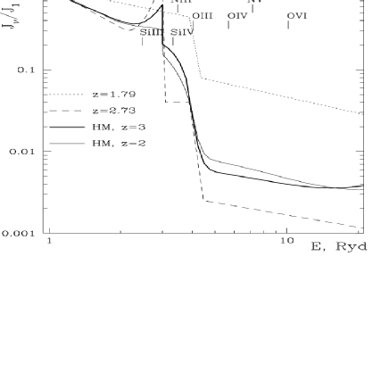
The angle-averaged intensity of the UV background determined by Haardt and Madau (1996) based on an earlier assessment of the QSO contribution is shown in Fig. 9 at redshifts and 3. The steps in the background are produced by photoelectric absorption of the source radiation by intervening absorbers at the H and He Lyman edges. The comparison with the purely absorbing IGM estimate shows the formation of emission “horns” due to the reprocessing of ionizing radiation by the IGM into redshifted H and He Lyphotons. The redshifted He Lyphotons enhance the flux of H -ionizing photons as does the continuum emission resulting from direct recombinations to the ground levels of H and He . At higher redshifts, the UV background more strongly resembles the spectral shape of the sources because the opacity of the IGM becomes so large that the UV background is increasingly dominated by local sources.
Combining Eq. (40) with Eq. (63), the photoionization rate may be expressed in terms of the emissivity as
| (73) |
where is the emissivity at the Lyman edge, is the spectral index of the UV background just shortward of the Lyman edge, is an effective lengthscale over which the distribution of sources contributes to the radiation field at any given point, the photoionization cross-section is approximated as , and is Planck’s constant. It is well known that in a uniform infinite Euclidean universe with point sources of radiation distributed throughout, the effective lengthscale is infinite and the local radiation field diverges (Olber’s paradox). Cosmological effects, in particular the finite age of the sources and the effects of redshifting, will guarantee convergence, and describes an effective horizon to the sources. Attenuation by a photoelectrically absorbing IGM will shorten the effective length even further, and will dominate at high redshifts. These two extremes, a cosmologically limited lengthscale and an attenuation limited lengthscale, may be combined into the approximate expression , where is the lengthscale limitation due to cosmological expansion and the finite age of the sources,and is the lengthscale due to attenuation by the IGM. For sources turning on at with (comoving) emissivity parametrized as , the effective (proper) horizon to the sources is
| (74) | |||||
for large Meiksin and White (2003). Values for the attenuation length are provided by Meiksin and White (2004) based on numerical simulations (see § VI.3.1). The values obtained lie between the medium and high attenuation models of Meiksin and Madau (1993) derived from direct absorption line counts.
Resulting values for the QSO contribution to the H ionization rate are given in Table LABEL:tab:GammaHI at selected redshifts. The estimates are derived from the QSO emissivities of Meiksin (2005) and Hopkins et al. (2007) using Eq. (73) and the attenuation lengths from Meiksin and White (2004), allowing for an extrapolation of the measured Lyman Limit System distribution to (see § VI.3.1 below). Results for both the Pure Luminosity Evolution model and the Pure Density Evolution models of Meiksin (2005) for the QSO luminosity function are given. The estimate based on the QSO luminosity function of Hopkins et al. (2007) uses the emissivity shown in their Figure 11. All the estimates agree within the errors.
| 1 Myr | 20 Myr | 100 Myr | 300 Myr | 900 Myr | |
|---|---|---|---|---|---|
| 0.02 | 2.7 | 4.9 | 6.2 | 6.7 | 6.8 |
| 0.001 | 2.6 | 4.6 | 6.2 | 6.9 | 7.5 |
Star-forming galaxies are an important potential source of ionizing radiation. While the spectra are likely too soft to produce appreciable He -ionizing photons, the hot young stars in star-forming galaxies could in principle provide even more hydrogen-ionizing photons than QSOs. An estimate of the contribution of star-forming galaxies to the UV background requires making a variety of assumptions regarding the Initial Mass Function, populations and ages of the stars as well as the numbers of faint galaxies below the survey limits. Some of these uncertainties are mitigated by using the results of galaxy surveys that measure the intrinsic flux from the galaxies close to the Lyman edge (the range Å is typical), since the stars that produce the ionizing radiation are the same as those dominating the detected light of the galaxies Madau et al. (1999). Even then, however, uncertainties in the spectra of the massive stars that dominate the radiation at early times introduce a comparable level of uncertainty into the estimate of the combined ionizing emissivity from the galaxy population Bruzual and Charlot (2003). Estimates for the conversion between the measured flux at 1500Å (restframe) and the predicted flux shortward of the Lyman discontinuity are provided in Table LABEL:tab:flux-convert assuming a Salpeter Initial Mass Function with and and either solar () or 1/20 solar () metal abundances, based on the STARBURST99 models of Leitherer et al. (1999).171717The code and model results are available at http://www.stsci.edu/science/starburst99/. A similar value of is quoted by Madau et al. (1999). The values for the ratio are about 5–10% larger, and for about 5–10% smaller, than the values in Table LABEL:tab:flux-convert. The lower mass cut-off appears appropriate for some starbursts; in any case, choosing a lower value only alters the normalization to the total star formation rate as the lower mass stars contribute negligibly to the spectra except at very late times Leitherer and Heckman (1995).
Another major uncertainty is the escape fraction of ionizing radiation, as this must multiply the emissivity based on galaxy counts and finally governs the contribution of the star-forming galaxies to the UV background. There are few direct measurements of the escape fraction, and virtually all are upper limits. Putman et al. (2003) infer a global escape fraction from the Milky Way of 1–2% from H spectroscopic measurements of nearby high velocity clouds. Based on a detection of Lyman continuum flux from FUSE observations of a local starburst galaxy, Bergvall et al. (2006) suggest an escape fraction of , subject to spectral modeling uncertainties. Fernández-Soto et al. (2003) place an upper limit of 4% for galaxies in the redshift range . Similar upper limits based on FUSE observations were obtained by Heckman et al. (2001) and Deharveng et al. (2001). Shapley et al. (2006) report the detection of UV radiation shortward of the Lyman edge in a sample of Lyman Break Galaxies at with a corresponding escape fraction of 14%, although the estimate is sensitive to the assumed calibrating population synthesis models and corrections for the IGM optical depth, and it may also apply only to the more luminous galaxies.
In addition to direct observational constraints, several attempts have been made to estimate the escape fraction from theoretical models allowing for inhomogeneities in the interstellar medium of galaxies, the influence of supernovae, and the flow of ionizing radiation through chimneys produced by large scale outflows Dove and Shull (1994); Dove et al. (2000); Wood and Loeb (2000); Ciardi et al. (2002); Clarke and Oey (2002); Fujita et al. (2003). Escape fraction values ranging from less than 1% for quiescent disks to more than half in an inhomogeneous IGM are obtained. The models suggest that high star formation rates, such as in Lyman Break Galaxies, may sufficiently fragment the interstellar medium of the galaxies and/or create sufficient channels through supernova-driven superbubbles that escape fractions in excess of 10% may be achieved, particularly if star forming regions are distributed throughout the disk of a galaxy.
A composite luminosity function of star-forming galaxies detected by the Lyman-break method181818The Lyman edge moves into the optical range at , permitting the identification of galaxies with large Lyman breaks, as is expected for galaxies with high star formation rates Leitherer et al. (1999). at was derived by Dickinson (1998). Madau et al. (1999) combined this with determinations of the Lyman-break population at by Madau et al. (1996) and Madau et al. (1998) to estimate the emissivity of star-forming galaxies and their contribution to the metagalactic UV background.
Establishing the star-formation history of the Universe is currently an area of intense activity. A revised UV luminosity function of Lyman Break Galaxies was provided by Steidel et al. (1999). Giavalisco et al. (2004) measured the luminosity density of Lyman Break Galaxies in the redshift interval , while Steidel et al. (2004) estimated the star-formation history of galaxies in the redshift interval . Yoshida et al. (2006) have measured the luminosity function of Lyman Break Galaxies in the SUBARU Deep Field at and 5. Bouwens et al. (2006) provide a comprehensive analysis of the UV luminosity function of galaxies at and the evolution of the luminosity function to .
Despite the heroic efforts to establish the UV luminosity density and cosmic star formation rates at high redshifts, the contribution of the galaxies to the metagalactic UV background is still uncertain due to several factors. In addition to the ionizing radiation escape fraction and UV-to-Lyman limit conversion factor, the effects of internal galactic extinction, uncertainty in the amount of intergalactic extinction by the IGM Meiksin (2006a) and the minimum source luminosity on the UV luminosity density and its evolution create further uncertainty in the net contribution of the galaxies.
The error budget may be illustrated using the results for Giavalisco et al. (2004); Bouwens et al. (2006). The uncertainty in the measured luminosity density of the sources is 20% or larger. Another factor of 3 uncertainty results from the uncertain extinction correction to the number counts Bouwens et al. (2006). The uncertain lower luminosity limit of the sources introduces a factor of 2 uncertainty to the integrated contribution of the sources to the UV background Bouwens et al. (2006). The conversion of the flux from the measured bands to shortward of the Lyman edge (see Table LABEL:tab:flux-convert) introduces at least another 20% uncertainty. The attenuation length is uncertain by about 30% Meiksin and White (2004), and the uncertain evolution rate and birth time of the sources introduces another 10% uncertainty in the effective length scale to use in Eq. (73). Since these uncertainties are primarily systematic, the factors must be multiplied. Altogether, taking middle values of the expected ranges still leaves a combined uncertainty of about a factor of 4 for the contribution of the galaxies to , excluding the uncertainty of the escape fraction.
Giavalisco et al. (2004) obtain for the comoving luminosity of sources at 1500Å, (in units of ) at and at Applying the conversion factors in Table LABEL:tab:flux-convert gives for the corresponding emissivities shortward of the Lyman edge at and at . Using these values in Eq. (73), combined with the attenuation length estimates of Meiksin and White (2004) (see § VI.3.1 below), gives at and at . Comparing with the required values for in Table LABEL:tab:GammaHI (see § VI.3.1), allowing for the contribution from QSOs in the PLE model of Meiksin (2005) (the PDE model estimates are even smaller), and allowing for a factor 4 uncertainty in the galaxy contribution imposes the restrictions on the escape fractions of at and at . Similar escape fractions are inferred by Inoue et al. (2006). Galaxies thus plausibly make up the missing ionizing radiation, but the uncertainties are still too great to preclude additional sources, which may actually dominate. Since re-radiation by the IGM itself may contribute some 20–40% of the total emissivity Meiksin and Madau (1993); Haardt and Madau (1996), these restrictions on may be further eased. The emissivities are based on source counts uncorrected for the effects of internal extinction on color. Corrections may increase the emissivities by as much as a factor of 3–4 Bouwens et al. (2006), corresponding to a similar reduction factor in the required escape fractions.
At , Bouwens et al. (2006) obtain a comoving integrated UV emissivity at Å of at , with the error range covering the uncertainty in the lowest luminosity of the contributing sources. Using the same procedure as above, this translates into the rather large ionization rate of . Correcting the colors for internal extinction increases this value by about another 50%. Consistency with the residual ionization rate at , after subtracting the QSO contribution (which is small), gives (or somewhat less, allowing for extinction corrections), a very plausible range, suggesting that these sources may in fact dominate the UV ionizing background at high redshifts.

IV.2 Fluctuations in the UV background
The discreteness of the sources of radiation will produce local fluctuations in the UV background. Several physical effects contribute to the fluctuations. Any single source will dominate the radiation field sufficiently nearby. The result is a region of enhanced photoionization around the source and a reduction in the local opacity of the IGM. Known as the “proximity effect,” the diminished strength of absorption by the Lyforest near an ionizing source like a QSO may be used to constrain the intensity of the UV background, as is discussed in the next section. If the opacity of the IGM to ionizing photons is sufficiently small that a large number of sources distributed over large spatial scales contribute to the radiation field, the fluctuations will be small. If the attenuation length, which is the characteristic distance over which the radiation from sources is diminished by IGM absorption, is smaller than the characteristic clustering scale of the sources, then the radiation field will be modulated by the large scale spatial distribution of the sources. In the limit of such a short attenuation length that the number of sources contributing to the radiation field in any given region is subject to large Poisson fluctuations, the radiation field will exhibit substantial fluctuations Zuo (1992a); Meiksin and White (2003). This will become a particularly appreciable effect near the reionization epochs of H and He , but may be an important effect well after the reionization epochs as well if the IGM opacity is sufficiently large at high redshifts.
The magnitude of the fluctuations may be estimated by considering the effect of Poisson fluctuations in the source numbers on the integrated intensity. The attenuation length is equivalent to the mean free path of an ionizing photon, the distance over which the mean number of absorbers encountered is unity. The probability that a photon survives a journey of a distance is then . In general the distance will depend on frequency, but most of the absorption takes place near the photoelectric edge at frequency . Provided the distances are sufficiently small that cosmological effects may be neglected, the generation of the radiation field may be considered in the Euclidean limit. Any individual source of luminosity a distance from a given location will then contribute a flux for . Allowing for a luminosity distribution function per unit luminosity per unit volume with mean spatial density of sources between minimum and maximum luminosities and of , and defining to be the mean number of sources within an attenuation volume, the distribution of the dimensionless energy density , where for a characteristic luminosity , becomes Meiksin and White (2003)
| (75) | |||||
where and is the normalized luminosity function of the sources
| (76) |
and . The function is given by
| (77) |
with defined implicitly through . For large , the distribution takes the asymptotic form , where is averaged over . It follows that the variance of the radiation energy density is undefined, diverging like for .
Examples of the resulting distribution function are shown in Fig. 10. A QSO luminosity function of the form Eq. (72) was used with parameters given by the maximum likelihood Pure Luminosity Evolution fit of Meiksin (2005) at (renormalized to ): , , , and at restframe Å. In anticipation of the discussion of helium reionization below (§ IV.3.2), the attenuation lengths were fixed at 7, 15 and 33 (proper) Mpc, corresponding to averages of 1, 10 and 100 sources per attenuation volume. When the average is small, the distribution becomes quite skewed towards low values, corresponding to few or no sources within an attenuation volume.
The Poisson fluctuations of sources within an attenuation volume will also give rise to spatial correlations in the radiation field. The correlation function is Zuo (1992b)
| (78) |
where the averages are performed over the dimensionless QSO luminosity function (eq. [76]). For the luminosity function above at , the coefficient , so that substantial correlations are expected on scales .
IV.3 Observational constraints on the UV background
IV.3.1 The proximity effect
The number of Lyforest systems decreases systematically near bright QSOs Murdoch et al. (1986); Tytler (1987b); Lu et al. (1991). The decrease, known as the “proximity effect,” is expected sufficiently near a QSO where its ionizing flux dominates the UV background Carswell et al. (1987). Bajtlik et al. (1988) quantified the effect in terms of the statistical properties of the Lyforest to obtain an estimate of the UV background.
The factor by which the H column density in an absorption system will be reduced is , where is the ratio of the ionization rate due to the QSO at a luminosity distance between the QSO and the absorber to the metagalactic ionization rate . The ionization rate due to the QSO is
| (79) | |||||
where is the observed flux from the QSO at frequency and is the luminosity distance to the QSO at redshift for a flat universe () Peebles (1993). For a power-law H column density distribution , the increase in intensity will decrease the number of absorption systems above a given threshold by the factor . A mean line density would then become
| (80) |
Measurements of as a function of distance from the QSO as inferred from the depression in line density permits a determination of the metagalactic .
Since Bajtlik et al. (1988), several estimates of the metagalactic ionization rate have been made using the proximity effect. Scott et al. (2000) performed a uniform analysis of the spectra of 99 QSOs at moderate resolution (Å) over the redshift range to obtain an estimate of over . (They also provide references to much of the previous literature.) The rates have generally exceeded the estimates of the contribution from quasars. Several systematic effects could account for some of the discrepancy. Redshifts for the quasars measured from low ionization permitted lines like the Balmer lines or Mg or from forbidden lines like [O ] Å are redshifted compared with Lyand C by a few to several hundred Boroson and Green (1992); Laor et al. (1995); Vanden Berk et al. (2001). If the higher redshifts reflect the true distances to the QSOs, then the QSO flux producing the proximity effect will be overestimated using QSO redshifts based on Lyor C , which in turn would result in an overestimate of the metagalactic ionization rate by as much as a factor of two Scott et al. (2000). Numerical simulations suggest that enhanced large-scale structure in the vicinity of a QSO will partly compensate for the photoionizing influence of the QSO, again resulting in an overestimate of the metagalactic rate by as much as a factor of 2–3 Faucher-Giguère et al. (2008a).
Quasar variability will introduce scatter in the estimates for and degrade the fit of against for a model assuming a constant quasar flux Bajtlik et al. (1988). Episodic behavior of QSO luminosities could introduce a further systematic in the estimates of the metagalactic ionization rate. If a QSO satisfies a survey magnitude threshold as a result of entering a bright phase, the neutral fraction will lag behind, resulting in an overestimate of the metagalactic rate. From Eq. (45) for , it follows that the actual metagalactic rate is a factor smaller than the estimate assuming equilibrium, where is measured from the deficit in Lyforest absorption lines near the QSO and . Time-averaging over a period during which the QSO is sufficiently bright to enter the survey produces the average factor . For s, this would result in too low a value for , and so too little suppression of the Lyforest line density over a distance from the QSO, as is frequently found Scott et al. (2000). An overestimate of the metagalactic photoionization rate by several percent could result.

IV.3.2 Constraints from helium ionization
The ratio of He to H column densities places a constraint on the ratio of the metagalactic UV background at the He and H photoelectric edges. From Eq. (42) and the corresponding equation for He , assuming the helium (like the hydrogen) is highly ionized and so almost entirely in the form of He ,
| (81) |
where and are the photoionization rates per atom of H and He , respectively. For an approximate temperature dependence of near K (and similarly for He ) and a hydrogen-to-helium number density ratio of 12.9, it follows from Eq. (81), Eq.(40) and the analogous equation for that
| (82) |
where the “softness parameter” is the ratio of the metagalactic UV energy density at the H and He Lyman edges Madau and Meiksin (1994), and and are the spectral indices just shortward of the respective edges. (Allowing for the full temperature dependences of the H and He radiative recombination rates introduces a weak temperature dependence of ; Shull et al. (2004).) Because of the steepness of at energies just above 4 Ry (Fig. 9), instead of the softness parameter, it is usually more convenient to introduce the ionization rate ratio , as it is this ratio which governs directly.
It follows from Eq. (18) that the ratio of the He to H optical depths at line center is given by
| (83) |
The value of is predicted to be large for a UV background dominated by QSOs (Fig. 9). For an intrinsic spectral index of , at , corresponding to Madau and Meiksin (1994); Haardt and Madau (1996), while for , , corresponding to Madau and Meiksin (1994). Interpolating to gives and . Additional photoionizing sources, like galaxies, will increase and further. The ratio of optical depths is thus expected to be large, so that a strong He Lysignature is expected from the IGM. The ratio also depends on the ratio of the Doppler parameters. For pure thermal broadening, it follows from Eq. (10) that , and will be quite large. But if velocity-broadening dominates (see Eq. [11]), then and . Systems optically thin in H Lywith as low as 0.1 will form saturated He Lylines.
Because of line-blanketing, the measured optical depths will scale according to Eq. (31). A large effective optical depth due to blanketing is expected Miralda-Escudé (1993); Madau and Meiksin (1994); Giroux et al. (1995). This has been confirmed by observations (see § II.2.5). The estimate of Madau and Meiksin (1994) requires for the 95% lower limit at of Hogan et al. (1997) if the absorbers are thermally broadened, but to reach the 95% upper limit of . For velocity-broadened absorbers, however, for which Zheng et al. (2004b) find evidence, the upper limit may be satisfied by . If the lower limit found by Heap et al. (2000) applies, however, then is required even for velocity broadened absorbers.
There is additional reason to believe values of occur at . While the detection of a high He Lyoptical depth was expected, the wide range in fluctuations in came as a surprise. Some of the systems indicate values as large as at based on follow-up optical observations of the H Lysystems corresponding to the He systems detected Zheng et al. (2004b); Reimers et al. (2005); Fechner et al. (2006). Combining measurements from FUSE observations over the redshift range with measurements of for the corresponding H systems using Keck observation, Fechner et al. (2006) obtain a very broad distribution for , as shown in Fig. 11. Systems detected in spectral bins affected by metal line absorption have been excluded. The systems are further restricted to those with line center optical depths in the range to assure completeness and reliable fits. Without this latter restriction, the full distribution ranges over . A trend of decreasing with decreasing redshift is also found Zheng et al. (2004b); Fechner et al. (2006). Only fluctuations producing an extremely soft spectrum with could account for the largest excursions. Such high values could arise from strong local H -ionizing sources, or from a broad distribution in the He -ionizing background with occasional low excursions. Higher values of are found in H voids, regions with Shull et al. (2004); Fechner et al. (2006), again consistent with a local overdensity of hydrogen-ionizing sources compared with He -ionizing sources producing the H voids. The trend is also consistent with an increase in the relative attenuation length of hydrogen-ionizing photons compared with He -ionizing photons, so that more distant hydrogen-ionizing (but not He -ionizing) sources are able to add to the radiation field in the H voids.
Monte Carlo realizations of the expected fluctuations in were performed by Fardal et al. (1998), allowing for the discreteness of the absorption systems and of the quasars. At , they find a range of values , peaking at . Since the He column density scales inversely with the local intensity of the UV background (provided most of the helium is ionized to He ), the contribution of source discreteness to the distribution in the He to H column density ratio may be predicted from Eq. (75) as , where .191919Because the H -ionizing radiation field will be much more narrowly distributed, its fluctuations will contribute much less to the fluctuations in and so may be neglected, except for large values due to the proximity effect. The joint H and He proximity effect would need to be modeled separately, including the effect on changing the attenuation length, which may be especially important for He -ionizing photons when the attenuation length and range of the proximity effect are comparable. The flattening of for shows that the average of is undefined, diverging logarithmically at the upper end due to regions of low ionization.202020The presence of diffuse radiation will limit the maximum values of , as will the approach to near full recombination to He . The maximum value, however, will still be so large that no average will be well-determined.
Using the distribution shown in Fig. 10 for an average of QSO sources per attenuation volume, the resulting distribution for is shown in Fig. 11. The distribution function shown by the solid line is computed as the average of two distributions matched to the measured distributions with mean and spread of at and at Fechner et al. (2006). The dashed line uses means increased by to and 2.06. The measured values are well described by the model, except for a small tail at . These values may be produced by patches of only partially ionized helium, as would remain during the epoch of He reionization before its completion Zheng et al. (2004b); Reimers et al. (2005). Alternatively, they may result from local H -ionizing sources reducing the H column density, but not the He . Effects of large scale structure and radiative transfer on the fluctuations were explored using numerical simulations by Maselli and Ferrara (2005), Bolton et al. (2006) and Tittley and Meiksin (2007) (see § VI.3.3 below).
The measured values for may be compared with the expectation for a UV background dominated by QSOs. By Eq. (82), the mean values for correspond to . From Eq. (73), . Approximating the emissivity as , taking Mpc from Eq. (105) below and Mpc for 10 QSOs in an attenuation volume at the He Lyman edge (§IV.2), gives for , producing a good match to the required average value of for a plausible emissivity spectral shape due to QSO sources.
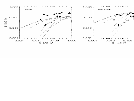
IV.3.3 Constraints from metal ionization
The presence of metal absorption systems permits further constraints on the shape of the UV metagalactic background. The ionization edges for several transitions of measured metal ions, primarily carbon, nitrogen, oxygen and silicon, lie in the energy range 1–10 Ry, as shown in Fig. 9. The measured column density ratios of ionized states of these elements have been used to distinguish a UV background dominated by hard sources like QSOs or Active Galactic Nuclei (AGN) from a background dominated by galaxies/stars Madau (1991). The inferred ionization fractions may also be used to convert the measured column densities of the detected ions compared with the H column density into physical densities, sizes and total metallicities Bergeron and Stasinska (1986); Donahue and Shull (1991); Bergeron et al. (1994). The findings suggest Lyforest systems have metallicities less than 0.01 solar, while Lyman Limit Systems have metallicities from less than 0.01 solar up to 0.1 solar. Some systems show evidence for multiple phases with densities different by at least a factor of 10 Bergeron et al. (1994). Sizes of typically tens of kiloparsecs are found, with total hydrogen densities of roughly .
Based on a comparison of Si to C vs C to C , Songaila and Cowie (1996) find systematically different behaviors for systems at compared with , as shown in Fig. 12. The Si to C ratio for a given C to C ratio cannot be satisfied for any softness parameter without enhancing the Si/C ratio to about 3. In this case, the high redshift systems require a break of a factor of 10 to 100 at the He Lyman edge, while little or no break is required by the lower redshift systems. The large break at is similar to the finding based on the He to H ratios found at discussed above. Refined estimates of the UV background, including a plausible contribution from starburst galaxies, suggest the Si/C ratio need not exceed twice solar Giroux and Shull (1997). Based on observations of metal systems at , Savaglio et al. (1997) and D’Odorico et al. (1998a) similarly find a much larger ratio of Si to C column densities compared with the expectation for a QSO or AGN dominated UV background. They find a large softness parameter between the He and H Lyman edges of is required to bring the overabundance of silicon over carbon to below a factor of 10 over solar.
Using 19 high quality QSO spectra over the redshift range , Schaye et al. (2003) and Aguirre et al. (2004) perform a pixel optical depth analysis of C , Si and H in conjunction with simulated spectra. They find evidence for a highly inhomogeneous distribution of carbon with a cosmic mean of at and no evidence for evolution over the redshift range , adopting the galaxy-QSO metagalactic spectrum of Haardt and Madau (2001), rescaled to reproduce the measured mean Ly transmitted flux. Introducing a large break in the metagalactic background at energies above 4 Ry, the He photoelectric threshold, for all redshifts indicates a decrease in metallicity with time, which could only be physical if large quantities of metal-poor gas were accreting onto the metal-enriched absorption systems or replacing them in the surveys as they accreted onto galaxy halos, possibilities that perhaps should not be discounted. Introducing the large break only at , as would occur if He were ionized late, however, yields a near constant (at most a weakly increasing with time) carbon abundance. They find no redshift evolution in the ratio , and the silicon and carbon data require no sharp spectral change in the UV background at . They find a strong correlation between and , and argue the redshift effect reported by Songaila and Cowie (1996) may result from a different range in probed as a function of redshift, possibly due to different quality spectra for samples at vs . They also infer a Si/C ratio of , with no indication for evolution in the ratio.
In a study of metal absorption systems in the spectra of QSOs with intervening C and O detections, Simcoe et al. (2004) find roughly 30% of the Lyforest is enriched to abundances below . The systems are adequately modeled using a UV background dominated by QSOs or AGN having a power-law source spectrum , assuming a solar abundance ratio of carbon to oxygen. If instead the absorption systems are overabundant in oxygen by , as found for metal-poor Galactic halo stars, then it is necessary to include a galactic radiation component.
Modeling metal absorption systems at using CLOUDY and an assumed UV metagalactic background with contributions from both QSO sources and galaxies, Simcoe et al. (2006) infer a trend of decreasing sizes and increasing densities from high to low ionization states. The largest, lowest density systems, with sizes of 0.1–10 kpc and densities of (in units of ), are seen exclusively in C or Si . These sizes are comparable to the minimum inferred sizes based on coincident absorption systems along neighboring lines of sight (§ II.2.6). The lower ionization species C and Si have sizes of 0.1–1 kpc and densities of , while Mg and Al systems have inferred sizes of about 100 pc and densities of . The smallest and densest structures are Fe absorbers, with sizes of about 1 pc and densities of .
Comprehensive analyses of metal absorption systems between that are optically thin at the H Lyman edge were carried out by Agafonova et al. (2005), Reimers et al. (2006) and Agafonova et al. (2007). They employ a Monte Carlo Inversion procedure which allows for a random distribution of gas density and velocity along the line of sight. The procedure assumes a constant metallicity for each system, that the gas is optically thin to the ionizing UV radiation, assumed uniform, and that the gas is in thermal and ionization equilibrium. The ionizing UV background is expressed in parametric form. All parameters of the model are then varied to obtain the best fit to the metal absorption features, using CLOUDY to compute the ionization states and temperatures. The method is described in detail by Levshakov et al. (2000), Agafonova et al. (2005) and references therein. Applied to individual systems, a range in He to H column densities is inferred from the data (Agafonova et al., 2005), suggestive of a variable UV radiation field. Since the variability is generally based on systems optically thick to He -ionizing radiation, the method does not distinguish between a UV radiation field that is variable on the metagalactic scale external to the absorbers and a radiation field that differs between the absorbers as a consequence of internal absorption.
These authors find a range of hydrogen densities from the analyses, with values as low as to as high as , similar to the findings of Simcoe et al. (2006). The line-of-sight sizes of the metal absorbers range from a few parsecs to over 100 kpc. Systems at are best fit by imposing a strong reduction in flux between 3 Ry and 4 Ry, as shown in Fig. 9. Such a reduction could be accounted for by strong He Lyabsorption. At , a much shallower break at 4 Ry is required compared with the model of Haardt and Madau (1996), suggesting there may be fewer high column density systems filtering the He ionizing radiation than assumed by the model. The radiation field at is dominated by sources with QSO/AGN spectra. Only a very small soft spectrum component from galaxies may contribute, suggesting an escape fraction of . Large fluctuations in the UV background are also required. At , these are likely produced predominantly by the effects of radiative transfer through an IGM optically thick to He -ionizing photons. The optical depth of He -ionizing photons is dominated by systems with , while much rarer systems with dominate the H -ionizing photon optical depth. As a result, the mean free path of He -ionizing photons is much shorter than for H -ionizing photons, and relatively fewer sources contribute to the He -ionizing radiation background in any given region. By , however, systems are sufficiently sparse that the IGM should become optically thin to He -ionizing radiation to large distances, and the fluctuations are instead likely produced predominantly by the spread in the spectral indices of quasars. Fluctuations in and an anti-correlation between and may be accounted for by the filtering through the IGM of radiation from QSO sources with a variety of spectral shapes and by differences in the mean densities of the absorbing clouds. The progressive hardening of the UV background towards lower would also account for the decrease in the median values for as decreases Zheng et al. (2004b); Fechner et al. (2006).
The modeling has some limitations, especially for systems with large values of . A system with is optically thin to H -ionizing radiation but thick to He -ionizing radiation, so that a break at 3–4 Ry must be introduced to account for the radiative transfer internal to the system. The assumption of thermal equilibrium assumes adiabatic cooling or heating are negligible. The timescales are also long for the more rarefied systems. For a temperature of K, the cooling time due to radiative recombination to H exceeds yr for , which is becoming long, particularly if flows occur on shorter timescales so that adiabatic gains or losses are not negligible. Simcoe et al. (2004) also point out that the O abundances are sensitive to the poorly determined soft x-ray background. Still, the studies have lent considerable insight to the physical nature of the metal absorption systems and the background UV radiation field that ionizes them.
V Early Models
Several models have been suggested for describing the physical structure of the Lyforest absorption systems. All of the early models have been supplanted by numerical cosmological simulations, which provide a largely successful description of the Lyforest and associated absorption systems within the broader context of cosmological structure formation. Vestiges of the early models, however, survive. In this section, elements of those models are discussed that continue to provide physical insight into the findings of the simulations, or which may still offer viable alternative descriptions of some absorption systems.
V.1 Pressure-confined clouds
The earliest physical model for the absorbers was one in which the absorption features arise from distinct clouds pressure-confined by a hot IGM Sargent et al. (1980). Denoting the cloud temperature and hydrogen number density by and , and those of the IGM by and , the condition of pressure equilibrium is . Allowing for clouds photoionized by a QSO/AGN-dominated UV background, small enough to be Jeans stable and able to withstand thermal evaporation by the hot confining medium, while requiring the IGM to meet the Gunn-Peterson constraint, Sargent et al. (1980) found for the cloud parameters at , , K, and K. These values were somewhat modified by Ostriker and Ikeuchi (1983) and others.
The pressure-confined models suffered from a serious shortcoming: a wide range of sizes was required to reproduce the range in observed H column densities. The higher column density systems would need to be so large that they would become unstable under their own gravity. Jeans stability limits the size of a self-gravitating cloud of density and temperature to be sufficiently small that a sound wave can cross it in less than the time for it to gravitationally collapse. This requirement is necessary to ensure the internal gas pressure gradient of the cloud is able to balance its weight. For an isothermal gas, this corresponds to a maximum size of
| (84) | |||||
In ionization equilibrium with an ionization rate , Eq. (44) gives a neutral hydrogen density for a cloud at K of . This gives a maximum column density for a Jeans stable cloud of . The observed distribution extends to values two orders of magnitude larger before the absorbers become Lyman Limit Systems. A further failure of the model is that a system with a column density of would have a typical size of 17 kpc. This conflicts with the sizes inferred from coincident absorbers along neighboring lines of sight to lensed QSO images, which give cloud sizes in excess of 70 kpc for systems with (§ II.2.3).
Elements of the pressure-confined model, however, may still describe some absorption systems. The clouds could, for example, be confined by a wide range of pressures in different environments, which are themselves gravitationally confined Baron et al. (1989). The association of metal absorption systems with galaxies suggests they may be pressure-confined systems within galactic halos, as may be Lyman Limit Systems Mo and Miralda-Escudé (1996).
V.2 Dark matter minihalos
A more viable physical model for the absorbers is gravitational confinement by a dark matter halo. Rees (1986) recognized that the Lyforest is a necessary consequence of the Cold Dark Matter (CDM) scenario for structure formation. The same normalization of the CDM primordial matter power spectrum that recovers the clustering of galaxies predicts an abundance of low mass minihalos with virial velocities comparable to the sound speed of photoionized gas. The gas trapped in these halos will produce absorption features with H column densities and line widths comparable to those observed Ikeuchi (1986); Rees (1986).
To fix parameters, consider the formation of a minihalo through gravitational collapse. The formation of a dark matter halo may be approximated by the spherical collapse model. The evolution of the radius of a spherical shell of mass in an Einstein-deSitter universe, which provides a good description at high redshifts, is given by the parametric solution Peebles (1980)
| (85) |
where is the virial radius of the shell and is the circular velocity of the shell at the time of virialization. For a top hat initial spherical perturbation, the central dark matter density at the time of virialization is , where is the critical Einstein-deSitter density at the virialization epoch at redshift . Since the gas is dissipative, its core radius will be smaller than the virial radius of the dark matter halo. Approximating the gas as being in hydrostatic equilibrium within a uniform density dark matter halo, the gas will have a gaussian profile with core radius
| (86) |
where is the gas temperature in units of K. A minihalo virialized at will be only a few kiloparsecs in size. A minihalo of mass would have an adequate circular velocity to confine the gas. The H column densities produced will range roughly over . Higher column density systems become self-gravitating and Jeans unstable Meiksin (1994), and will likely produce stars.
Bond et al. (1988) point out that the gas will in general be in a dynamical state, either collapsing with an increasing core density or expanding after photoionization. The observational signatures and thermal properties of minihalos were explored by Meiksin (1994). Gas associated with the minihalos gives rise to absorption features with on scales of 100 kpc at . Even though the gas is in motion, the line profiles are found to remain nearly Doppler in shape, although broadened by the gas motion. In the idealized case of an isothermal gas in free expansion, so that the gas profile is gaussian with a linear velocity profile , the Voigt profile is exactly preserved for lines of sight passing through the cloud, but with the Doppler parameter broadened to . Typical temperatures in the inner region of minihalos with circular velocities of , which give rise to systems with , are K, consistent with the measurements of Rauch et al. (1996) for metal absorption systems expected to be associated with comparable H column densities (see § II.2.6 above). In the inner 10–30 kpc, temperatures of K are predicted, with substantial deviations from thermal equilibrium due to adiabatic heating of the infalling gas. In the outer 10–100 kpc, the gas is significantly adiabatically cooled by Hubble expansion. Temperatures half these values are expected in smaller halos of .
Further consequences of the minihalo model, including number counts, effects of photoionization, and ablation due to ram pressure on minihalos moving relative to their environments, have been explored by Ikeuchi et al. (1989a, b), Murakami and Ikeuchi (1990), Miralda-Escudé and Rees (1993), and Murakami and Ikeuchi (1993, 1994).
V.3 Caustics and sheets
A gravitational perturbation will generically form sheets since the enhanced density along a given direction will accelerate the collapse along that direction. Once a growing density fluctuation becomes non-linear, it will produce a caustic. The caustic formation is well-described by the Zel’dovich approximation Zel’dovich (1970)
| (87) |
where is the comoving position of a particle with initial comoving position , is the peculiar velocity, describes the initial deformation of the density field, the gradient is with respect to , and is the growth factor for linear perturbations Peebles (1993). The physical radius is related to the comoving radius through , where is the expansion factor of the Universe at the epoch corresponding to redshift . Conservation of mass gives for the density, up until the time of caustic formation, , where the denominator is the determinant of the Jacobian of the coordinate transformation. For 1D collapse, the density prior to caustic formation grows as , which is exact for the 1D collapse of a slab. Gravitational instability ensures that a uniform density ellipsoidal density perturbation will collapse most rapidly along its shortest axis, forming a “Zel’dovich pancake.”
Baryons infalling along with the dark matter will produce Lyforest absorption features. The line profiles will become distorted at the time the caustic forms before the baryons come into dynamical equilibrium McGill (1990); Miralda-Escudé and Rees (1993); Meiksin (1994). The H column densities produced will range over about , with postshock temperatures peaking at K Meiksin (1994).
V.4 Galactic models
Ever since the earliest papers on the Lyforest, it was recognized that galaxies should give rise to intervening absorption systems. Their characteristics and frequency, however, are unclear. The interstellar medium of disk galaxies is expected to produce damped Lyforest absorbers, although relatively few DLAs have been shown to arise from disks (see § VIII.1.1 below). Other suggestions include condensates in cooling outflows from dwarf galaxies Wang (1995), the gas-rich dwarf galaxies themselves York et al. (1986), debris from satellite galaxies lost through tidal stripping by a central galaxy or expelled by supernovae Wang (1993); Morris and van den Bergh (1994), or pressure-confined clouds in a two-phase gaseous galactic halo medium Mo and Miralda-Escudé (1996). The outflow model in particular may give rise to distorted absorption line features if a line of sight intercepts the outflowing diffuse gas.
Another suggestion is that the absorption lines arise from gas in extended disks with too low surface density to produce many stars, the “Vanishing Cheshire Cat” model of Salpeter (1993). In this model, an inner disk gravitationally-confined region of radius about 15 kpc is surrounded by an extended pressure-confined disk of radius about 250 kpc. The inner region has a low gas surface density compared with most disk galaxies, but sufficiently large to produce a DLA feature in any line of sight passing through it. The outer region has such a low surface density that the hydrogen is photoionized by the metagalactic UV background. The outer region will give rise to Lyforest features. A transition region will produce Lyman Limit Systems. The relative abundances of the various H column densities is accounted for by the progressively diminishing geometric cross section for increasing column densities. The transition between gravitational confinement and pressure confinement may be adjusted to account for deviations from a perfect power law in the column density distribution. The “Cheshire Cat” nature of the galaxy arises once star formation begins, producing a starburst galaxy. Metal-enriched gas ejected by the stars will accelerate the cooling and strengthen the burst, resulting in the expulsion of the gas in the central region and quenching further star formation. The result will be an outer “smiling” gaseous disk, possibly enriched in gas and metals by a galactic fountain if material from the starburst falls onto the disk, and a very low surface brightness “invisible” galaxy in the center.
VI Numerical Simulations
VI.1 Cosmological structure formation
VI.1.1 Dynamical evolution of the dark matter and baryons
The successful description of the large scale distribution of galaxies by the Cold Dark Matter dominated scenario of cosmological structure formation Davis et al. (1985) led to attempts to account for the Lyforest within the same scenario. Using a combined hydrodynamics and gravity code, Cen et al. (1994) demonstrated that the baryons will trace similar small scale structure as does the dark matter due to gravitational instability in the Cold Dark Matter scenario. Several other groups soon followed with similar results Zhang et al. (1995, 1997); Hernquist et al. (1996); Miralda-Escudé et al. (1996); Wadsley and Bond (1997).
In the gravitational instability scenario of structure formation, cosmological structures grow from smaller structures through gravity. The growth of structures is governed by the coupled gravity-fluid equations describing both the collisionless gravitating matter component and the collisional baryonic component. Because of the enormous change in spatial scales as the Universe expands, it is most convenient to solve the equations in a frame comoving with the expansion Peebles (1993). The physical position and velocity are then expressed in terms of the comoving position and peculiar velocity according to
| (88) |
where and is the cosmological expansion factor corresponding to the cosmological epoch at the redshift .
The dynamical equations for the dark matter component are
| (89) | |||||
| (90) |
where is the gravitational potential, and the gradient is with respect to the comoving coordinate system. The fluid equations expressing mass and momentum conservation are
| (91) | |||||
| (92) |
where and are the gas density and pressure at at cosmological time . Because the evolution equation for the entropy, Eq. (51), is already in the comoving frame, it remains the same with the understanding that is replaced by Peebles (1993). The heating and cooling terms include the physical processes discussed above in § III.2. The evolution of the ionization state of a mixture of hydrogen and helium is given by Eqs. (46). The inclusion of ionization assumes a given set of H , He and He photoionization rates and photoheating rates. These must be computed from the ambient radiation field. The initial ionization state of the gas is set during the passage of ionization fronts produced by the radiation sources that photoionized the gas during the epochs of hydrogen and helium reionization. This is discussed in § VII below.
The dark matter and fluid are coupled through Poisson’s equation for the gravitational potential
| (93) |
where is the total mass density of the dark matter and fluid combined, is the spatial average of over the Universe, and has been assumed. In terms of the present day matter closure parameter , . Eqs. (89) – (93) are valid for any Friedmann-Robertson-Walker universe, including those with non-zero vacuum energy (such as an effective cosmological constant).
These are the same equations that describe the mix of dark matter, baryons and radiation that give rise to the Cosmic Microwave Background, except for the addition of the radiation energy density and pressure. The principal difference is that while the density fluctuations are linear for the CMB up to the time the baryons begin to recombine and decouple from the radiation, the description of the growth of cosmological structures extends the computation of the fluctuations into the nonlinear regime. Numerical solutions to Eqs. (89) – (93) generally begin at a sufficiently high redshift that the primordial density fluctuations are still linear on the scales of interest, but after the matter and radiation have decoupled. The most convenient set of boundary conditions for solving the PDEs for the coupled dark matter and gas on cosmological scales is to assume all the variables are periodic over the simulation volume. It is therefore important that the simulation volume be sufficiently large to represent a fair sample of the Universe.
No structures will form unless the matter is initially inhomogeneous. The inhomogeneity is usually specified in terms of a primordial power spectrum of matter fluctuations, which is the ensemble average of the squared modulus of the Fourier modes of the density field. The mass density expanded in Fourier modes within a periodic Cartesian volume may be expressed as
| (94) |
where the Fourier amplitudes are assumed to have random phases and to be distributed according to a gaussian random process. The power spectrum, which quantifies the amplitude of the density fluctuations, may be defined as , where the average is over independent statistical realizations of the Fourier amplitudes.
The real space analogue of the power spectrum is the spatial correlation function of the density field
| (95) |
where the average is carried out over all spatial locations . The correlation function is related to the power spectrum through a Fourier transform
| (96) |
where is the mean spatial density of the particles, and the Poisson noise contribution due to an average number of particles per simulation volume has been subtracted.
It is convenient to define the amplitude of density fluctuations
| (97) |
The amplitude of mass fluctuations in a sphere of radius is then given by
| (98) |
where is a spherical Bessel function. A common fiducial normalization measure is the mass fluctuation filtered on a scale of Mpc, where . The spectrum of matter fluctuations may be expressed in the form
| (99) |
where is the transfer function describing the evolution of density perturbations as they cross the present-day horizon scale with amplitude , is the spectral index, and is the growth factor for the density perturbations (see § V.3). The transfer function for a Cold Dark Matter dominated universe was first computed by Peebles (1981). A fast numerical code for computing the transfer function to high accuracy is provided by Eisenstein and Hu (1999).
VI.1.2 Methods of numerical simulations
Several numerical methods have been developed for solving the combined gravity-fluid equations. The most common methods for solving the dark matter evolution equations sample the distribution function of the dark matter using massive pseudo-particles and solve for their evolution either on a mesh or using a hierarchical tree. The most common mesh codes use either the Particle-Mesh (PM) or Particle-Particle Particle-Mesh () techniques. Tree algorithms instead arrange the particles into a hierarchy of groups and approximate the forces exerted by distant groups on a given particle by their lowest multiple moments. The fluid equations are frequently solved using a finite-difference representation of the fluid equations, handling shocks either with artificial viscosity or through shock capturing. An alternative scheme, Smoothed Particle Hydrodynamics (SPH), smooths the fluid equations and samples the smoothed fluid variables using pseudo-particles. The algorithm is intrinsically Lagrangian in nature. A comparison of two popular publicly available codes using these methods, ENZO and GADGET, is provided by O’Shea et al. (2005). The paper also serves as a good entry point to the vast literature on the subject. A more general overview of -body methods is provided by Bertschinger (1998).
All of the techniques share a common method for initiating the density fluctuations and associated peculiar velocity field based on the Zel’dovich approximation Efstathiou et al. (1985). Substituting , using Eq. (87) for the dark matter, into the equation for peculiar velocity from Eq. (90) gives
| (100) |
after noting that , which follows from Eq. (91) applied to the combined dark matter and gas density. The initial deformation is therefore proportional to the gravitational potential (up to an arbitrary integration constant). This offers a straightforward prescription for specifying the initial conditions. First, choose the ’s according to a gaussian random process: , where is a gaussian random deviate between with zero mean and unit variance, and is a random phase uniformly distributed over . In Fourier space, the gravitational potential is since the Fourier transform of is , where is the Fourier transform of . The gravitational potential may then be constructed from
| (101) | |||||
The deformation function then follows from Eq. (100). The displacements and velocities of the particles then follow from Eqs. (87),
| (102) | |||||
| (103) |
The optimal form of these equations allows for convolution with the differencing operator used to evaluate the gradient of the gravitational potential Efstathiou et al. (1985). Once initiated, any of the various numerical methods described above may be used to evolve forward the dark matter and baryon fluctuations into the nonlinear regime.
The resolution requirements of the simulations depend on the statistical quantity for which convergence is sought. While the demands for convergence on the H column density distribution over the range are not very severe, the early simulations tended to over-estimate the width of the absorption features. It is now recognized that good convergence on the Doppler parameter distribution and of the pixel flux distribution requires at the minimum good resolution of the Jeans length Theuns et al. (1998); Bryan et al. (1999). A resolution of kpc (comoving) is about the right level at , but still inadequate by Bryan et al. (1999), although the rate of convergence is sensitive to the gas temperature and assumed cosmology. Slightly coarser resolution is adequate for converging on the pixel flux distribution. A large simulation volume is required to ensure that the full contribution of long wavelength modes is included Wadsley and Bond (1997); Theuns et al. (1998); Bryan et al. (1999), requiring a box size of at least Mpc (comoving). Similar demands are found using pure dark matter pseudo-hydrodynamics simulations, for which sequences of large high resolution simulations have been performed to test convergence Meiksin and White (2001). Matching both the resolution and box size requirements demands simulations of minimally zones, and preferably zones for grid based codes to achieve good convergence on the properties of low H column density systems. Similar numbers of particles are required for SPH computations. Even with these parameters, converging on the extremes in the temperature distribution proves difficult. Such large hydrodynamics simulations are only now becoming feasible.
The simulations show that the baryons closely trace the distribution of dark matter down to the Jeans length scale, when pressure forces prevent further collapse of the baryons. This has prompted an alternative approach to IGM simulations based solely on the evolution of the dark matter Petitjean et al. (1995); Croft et al. (1998); Meiksin and White (2001). The gas overdensity is either set equal to the dark matter overdensity or by allowing for a pressure by treating it as a modification to the gravitational potential in the Hydrodynamics Particle Mesh (HPM) approach Gnedin and Hui (1998). The gas temperature is either solved for allowing for photoelectric heating and radiative cooling Petitjean et al. (1995) or through a polytropic equation of state . This alternative is based on the recognition by Hui and Gnedin (1997) that the temperatures found in numerical hydrodynamics simulations are determined largely through a balance between photoelectric heating and adiabatic cooling losses for structures with overdensities . Comparisons with full hydrodynamical computations show that using a PM code or HPM code with a polytropic equation of state gives a reasonably good description of the properties of the IGM, including its absorption statistics Meiksin and White (2001); Viel et al. (2002, 2006), although full hydrodynamics simulations should still be used for detailed comparisons to the data.
Yet another approach altogether is to generate the density fluctuations stochastically from a lognormal distribution Bi et al. (1992); Bi (1993); Bi and Davidsen (1997). This approach captures many of the qualitative features of the structure of the IGM, and provided an early argument that the Lyforest itself may be accounted for by density fluctuations in a diffuse IGM.
VI.2 Physical properties of the intergalactic medium
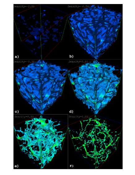
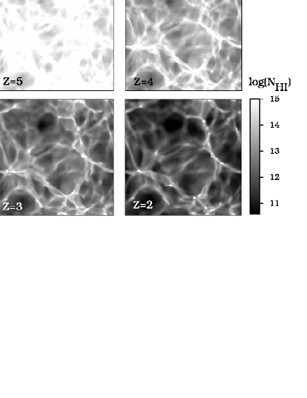
The results of structure formation simulations show that the IGM fragments into an interconnected network of sheets, filaments and halos Cen et al. (1994); Zhang et al. (1995); Katz et al. (1996); Miralda-Escudé et al. (1996); Wadsley and Bond (1997). The various morphologies correspond to different physical densities and different H column density absorption systems. These dependences are illustrated in Figures 13 and 14, taken from the simulation of Zhang et al. (1998) of a Cold Dark Matter dominated Einstein-deSitter universe with the radiation field from Haardt and Madau (1996) based on QSO sources. The simulation volume was 9.6 Mpc (comoving) on a side, and the power spectrum was normalized to with used. At , systems with arise from the amorphous underdense regions enclosed by the sheets. The underdense regions have characteristic diameters of a few comoving Mpc, and occupy most of the volume of the Universe. The sheets have densities comparable to the mean baryon density, and give rise to absorption systems with . Systems with originate in the filaments, which are moderately overdense structures (). Higher column density systems, with , arise in spheroidal nodes with overdensities of several to over a hundred embedded within the filaments.
The mean temperatures of overdense systems range over to Cen et al. (1994); Zhang et al. (1998); Theuns et al. (1998), while Miralda-Escudé et al. (1996) find mean temperatures up to . These larger values may be due to the hard UV background assumed. Much higher temperatures are also found, extending up to K, for gas associated with collapsed halos Theuns et al. (1998). There is less agreement on the temperatures in the underdense regions. The time to achieve thermal equilibrium exceeds a Hubble time for underdense gas Meiksin (1994); Miralda-Escudé and Rees (1994). The gas temperature will therefore reflect the thermal history of the gas following reionization, and so is sensitive to the particular reionization model. The Lyforest simulations also did not take into account the heating effects of reionization itself Tittley and Meiksin (2007).
The thicknesses of the filaments are approximately 100 kpc (proper), with coherence lengths of about a Mpc. The scales are consistent with the observational constraints based on neighboring line-of-sight statistics discussed in § II.2.3 above. This is comparable to the isothermal Jeans length. For a characteristic hydrogen number density of , corresponding to 5 times the mean baryon density at , and a characteristic temperature of K, the pressure is and the Jeans length from Eq. (84) is 320 kpc.
The baryonic overdensity at is found to scale roughly as , with the neutral fraction scaling as Zhang et al. (1998). The neutral fraction dependency is comparable to the estimate in § II.2.3 above, and results in virtually all the baryons’ residing in the Lyforest at .
The structure of the IGM at differs somewhat from its structure at . Davé et al. (1999) obtain the relation between overdensity and H column density of , similar to the finding of Zhang et al. (1998) at . A given overdensity results in H column densities smaller by a factor of 10–50 at than at . Most absorption systems at low redshift arise in systems with hydrogen densities of for H column densities of . Structures retain coherence over scales of several hundred kiloparsecs. The gas temperatures for structures with are about a factor of 2 smaller at than at . A hot, intermediate-density gas phase also arises from shocks in filaments and in galaxy, galaxy group and galaxy cluster halos, reaching temperatures of over K.
VI.3 Statistical properties of the absorption systems
VI.3.1 Mean metagalactic ionization rates
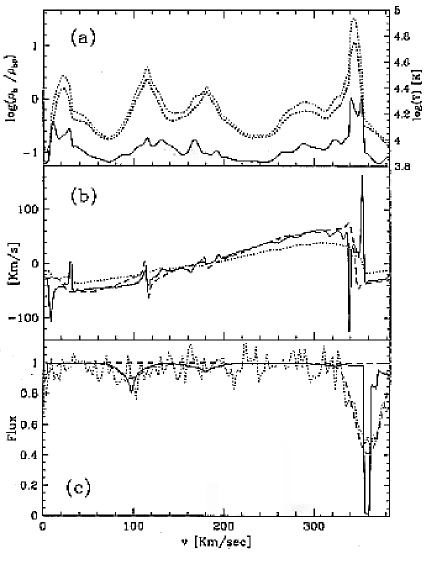
Almost all that is directly known about the structure of the IGM is derived from spectra. The simulation results must therefore be translated into spectra for comparison against observational data to test the validity of the models. The spectra, normalized to a unit continuum level, may be expressed as , where , the IGM optical depth as a function of frequency, is given by Eq. (14). Allowing for a peculiar velocity varying along the line of sight,
| (104) |
Setting , where is the local density contrast, Eq. (104) is identical to Eq. (15) for the Gunn-Peterson effect in the absence of perturbations (). For this reason, the varying optical depth of the IGM is sometimes referred to as giving rise to a “fluctuating Gunn-Peterson effect” Miralda-Escudé and Rees (1993); Cen et al. (1994).
An example of a spectrum generated from the CDM simulation of Cen et al. (1994) with , , , and normalization is shown in Figure 15. The temperature variations closely trace the baryon density fluctuations. The absorption features are slightly offset from the density features due to the peculiar motion of the gas. Mild overdensities produce weak features while large overdensities produce stronger features. The apparently isolated absorption features arise not from distinct clouds but from modulations in the density field produced by the gravitational instability of primordial density fluctuations.
Any comparison between the simulated and measured spectra requires normalization by the uncertain ionization rates for H and He . The uncertainty in the normalization rate for He is compounded by the unknown epoch of He reionization, which may have been as late as . Late He reionization will also affect the gas temperatures, particularly for underdense gas. This in turn affects the optical depth through the gas. Much of the uncertainty on global flux properties may be removed by normalizing to the measured mean Lytransmission of the IGM. Although an error in the temperature of the gas will result in a small offset in the inferred ionization rate (see Eq. [42]), once normalized, the probability distribution of the emissivity is only slightly affected. Altering the temperature of the gas as required by the line-widths, either directly or by boosting the heating rate, can further improve the fits.
Various groups have provided estimates for the H -ionization rate based on matching their simulation results to measurements of the mean Lytransmissivity. Results from Meiksin and White (2004), Bolton et al. (2005) and Bolton and Haehnelt (2007) are shown in Table LABEL:tab:GammaHI. All the predicted rates are in reasonably good agreement. Bolton and Haehnelt (2007) provide an additional estimate at of , which agrees well with the estimate from Tytler et al. (2004a) of . An additional uncertainty of a few to several percent may result from fluctuations in the ionizing background Gnedin and Hamilton (2002); Croft (2004); Meiksin and White (2004). A comparison of the required ionization rates with the predictions from QSO sources shows that unless there is a large population of low luminosity AGN so far undetected at high redshifts, QSOs alone are unable to provide the required ionization rates at .
Specifying fixes the entire equilibrium ionization structure of the gas (except in isolated optically thick regions). This permits the contribution of the IGM to the attenuation length of ionizing photons to be determined directly from a simulation. In principle, a self-consistent solution for the equilibrium structure of the IGM may then be obtained, including the magnitude of the required emissivity for any given spectral shape using Eq. (73). Meiksin and White (2004) find for a CDM cosmology the (proper) attenuation length is approximated to 10% accuracy by
| (105) |
for . Because the simulation underpredicts the number of Lyman Limit Systems by a large factor, these are added using the results of Stengler-Larrea et al. (1995). It is found that the diffuse gas comprising the Lyforest and the Lyman Limit Systems contribute about equally to the attenuation length, consistent with models based on direct line counts Meiksin and Madau (1993). The implied (comoving) metagalactic emissivity at the Lyman edge required to recover the H ionization rates is Meiksin (2005)
| (106) |
where and and is the spectral index of the metagalactic emissivity, . The errors on are the and limits.
VI.3.2 Spectral properties of the IGM
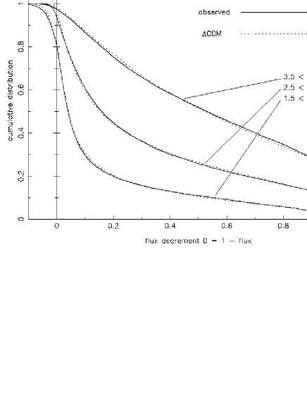
The predicted spectral properties of the Lyforest are sensitive to the cosmological parameters used Rauch et al. (1997b); Wadsley and Bond (1997); Theuns et al. (1999); Machacek et al. (2000); Jena et al. (2005). Comparisons with the spectral properties of the Lyforest have shown impressive agreement for plausible cosmological models. Machacek et al. (2000) show that the distribution of optical depth per pixel in the models is well-fit by a lognormal distribution for values between , roughly the measurable range. This prediction is confirmed by the observations of Becker et al. (2007), who find the flux distributions in 55 high resolution QSOs are well-reproduced by lognormal distributions for the underlying optical depths. Detailed comparisons show that the predicted cumulative distributions of pixel fluxes agree to a precision of a few percent with measurements in individual QSO spectra Meiksin et al. (2001).
These results suggest the Lyforest may be used as an effective tool for selecting between rival cosmological models of structure formation. An example of a comparison between the CDM simulation above and high signal-to-noise ratio high resolution Keck spectra of 7 QSOs is shown in Figure 16 Rauch et al. (1997b). Machacek et al. (2000) and Meiksin et al. (2001) find that the shape of the pixel flux distribution and the magnitude of the Doppler parameters vary systematically with the normalization on small scales, such as filtered on the Jeans scale, as defined by Eq. (98) with filter scale from Eq (84). A detailed comparison between the predicted flux distributions for several cosmological models and measurements from several high resolution Keck spectra constrains , defined for an isothermal gas at K, to the range at Meiksin et al. (2001), although this is somewhat subject to the uncertain thermal properties of the gas. The closest agreement is found for the larger values of . A range of CDM models, however, shows that agreement with inferred from WMAP measurements of CMB fluctuations prefers lower values Meiksin and White (2004), so that there is some tension between the higher normalization preferred by the Lyforest simulations and the lower normalization preferred by the CMB measurements.
Voigt profile fitting to the spectra permits comparison between the predicted and measured H column density and Doppler parameter distributions. Here the models fair somewhat less well compared with the pixel flux distribution. The models successfully reproduce the H column density distributions to good accuracy over a wide range of values of at high redshifts () Cen et al. (1994); Zhang et al. (1995); Hernquist et al. (1996); Zhang et al. (1997); Wadsley and Bond (1997); Meiksin et al. (2001) and at moderate to low redshifts () Davé et al. (1999); Paschos et al. (2008). A discrepancy is found at higher column densities, with simulations generally finding fewer systems with than measured. This is particularly true for Lyman Limit Systems Katz et al. (1996); Meiksin and White (2004), although extrapolating the simulation results to smaller mass halos suggests agreement is possible, depending on the appropriate minimum circular velocity of halos able to produce high H column density systems in the metagalactic photoionizing background Gardner et al. (2001). A smaller discrepancy is found for DLAs. The simulations of Nagamine et al. (2007) suggest the incidence of DLAs may be met if they are associated with halos having masses as low as .
It is less clear that all Lyman Limit Systems arise from collapsed halos. Allowing for radiative transfer effects, Kohler and Gnedin (2007) find their simulations produce Lyman Limit Systems from material bound to and falling onto galaxies rather than from minihalos. It is possible the systems have more than a single origin.
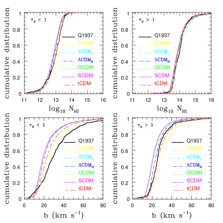
Because the detailed distribution of the absorption line parameters is sensitive to the method of line finding and fitting (see § II.2.1), a definitive comparison between the simulations and the measured absorption line properties requires identical line analysis methods. Automating the line analysis is necessary for processing the large number of lines of sight from simulations to build up reliable statistics. A few codes are publicly available. An industry standard is VPFIT,212121http://www.ast.cam.ac.uk/rfc/vpfit.html a sophisticated code that handles in addition to H features a wide range of metal lines. A simpler alternative well-adapted to automated fitting of H features is AutoVP Davé et al. (1997). Based on fits with AutoVP, Davé et al. (1997) find that the simulations predict a greater fraction of lower Doppler parameter systems than measured. Similar discrepancies were found by Bryan et al. (1999) and Theuns et al. (1999).
A detailed comparison between several high resolution QSO spectra and numerical simulations for a variety of models, analysed using AutoVP and a similar code, SPECFIT, by Meiksin et al. (2001) shows that it is not possible to match simultaneously the pixel flux distributions, column density distributions, and Doppler parameter distributions using simulations with optically thin reionization. While adjusting may help to match the Doppler parameters, it destroys agreement with the pixel flux distribution. In Figure 17, a comparison is shown between the predicted and measured line parameter distributions for the Lyforest detected in the spectrum of the QSO Q1937–1009. The systems have been isolated by their line center optical depths. The comparisons show that the discrepancies are due primarily to the low optical depth systems, with line center optical depths .
The origin of the discrepancies is most likely the temperature of the gas. Artificially broadening the absorption features gives excellent agreement between the measurements and predictions for the CDML model for the pixel flux and column density distributions, and good agreement between the Doppler parameter distributions. Since the optically thin absorbers arise in underdense regions, the temperature of the gas will retain a memory of its heating history. Since the underdense gas occupies most of the volume of the Universe, whatever heated the gas must have been ubiquitous. The best candidate is late reionization of He , in the redshift interval . This would boost the gas temperature, possibly by the required amount. The effects of heating by late He reionization may be mimicked to some extent by boosting the He heating rate Bryan and Machacek (2000); Tytler et al. (2004a), but the only fully satisfactory solution requires incorporating radiative transfer Tittley and Meiksin (2007).
With the goal of developing a physical description for the origin of the Doppler parameter distribution, Hui and Rutledge (1999) introduce a semi-analytic approach based on the growth of the density perturbations to derive a Doppler parameter distribution of the form
| (107) |
where is a fit parameter. Restricting their analysis to systems with column densities , corresponding to the physical conditions of the IGM for which their analysis best applies, Hui and Rutledge (1999) find the distribution provides statistically acceptable matches to the Doppler parameter distributions of the Lyforest along the lines of sight to four QSOs with high resolution Keck spectra Hu et al. (1995). Adequate matches, however, were not found for Q0000–26 Lu et al. (1996b) or HS 19467658 Kirkman and Tytler (1997a). The Doppler parameter distributions measured in the spectra of all six of the QSOs, without any restriction on the column density range applied, are well-fit by lognormal distributions (see Table LABEL:tab:bfit). Ricotti et al. (2000) generalize Eq. (107) to
| (108) |
where is a fit constant, and , and are allowed mild dependences on the column density. The best fits obtained for absorbers in several lines of sight over the redshift range have , and , with values almost independent of column density.
Several attempts have been made to infer the temperature of the IGM directly from the Doppler parameter distribution. One approach is to normalize the distributions using simulations, invoking additional sources of heat input to allow for a range in temperatures Bryan and Machacek (2000). Another exploits a polytropic relation between the gas density and temperature Hui and Gnedin (1997); Schaye et al. (1999), calibrated using numerical simulations. Both methods rely on numerical simulations that neglect the effect of reionization on the temperature of the underdense gas, which may be substantial Abel and Haehnelt (1999); Bolton et al. (2004); Tittley and Meiksin (2007). Modeling the Doppler parameter distributions according to Eqs. (107) and (108) to obtain lower cutoff values, Ricotti et al. (2000) and Schaye et al. (2000b) find evidence for a temperature jump and reduction in the polytropic index towards isothermality near . Both groups attribute their results to late He reionization. He reionization simulations predict a more gradual change McQuinn et al. (2008). No significant change in the temperature or polytropic index over the redshift range is found by McDonald et al. (2001, 2003). Although any conclusion using these methods is subject to the accuracy of the modeling assumptions made, the possibility of measuring an unambiguous temperature jump in this redshift range merits further investigation.
VI.3.3 Intergalactic helium absorption
As for the H absorption features, the numerical simulations predict the properties of He absorption as well. The systems that dominate the measured He optical depths arise from the diffuse structures in underdense regions Zhang et al. (1995); Croft et al. (1997). This makes predictions for the He optical depths difficult for two reasons: 1. high spatial resolution is required to accurately compute the structures in the underdense regions, and 2. the gas temperature is sensitive to the history of reionization since the time for the temperature to reach equilibrium is comparable to or longer than a Hubble time. The latter affects both the ionization fraction of He because of the temperature dependence of the radiative recombination rate and the Doppler widths of the absorption features. Another uncertainty is the epoch of full helium reionization. The results of Zhang et al. (1995) and Zhang et al. (1998) suggest matching to both the H and He Lymean optical depth measurements at requires an ionization rate ratio of , comparable to the inferred values from line statistics (§ IV.3.2) and corresponding to an intrinsic QSO spectral index of 1.8–2.0, allowing for filtering through the IGM Haardt and Madau (1996). A similar estimate is obtained from high resolution numerical simulations by Bolton et al. (2006), who find values for rising from at to at , assuming a spatially uniform UV background. Most of the uncertainty stems from the uncertainties in the measurements of the He Lymean optical depths. Allowing for spatial fluctuations in the QSO contribution lowers the inferred values for by about a factor of two. Allowing for fluctuations also reproduces much of the observed scatter in the He to H column density ratio (§ IV.3.2), except for the extreme excursions at and .
VI.3.4 Metal absorption systems
By providing the physical scales of density structures and their associated temperatures, the simulations permit estimates of the ionization states of metals for any assumed UV radiation field. Several observed features are reproduced by the models. The metal absorption features arise within the substructure of systems that give rise to the H Lyfeatures, and may result in multiple features corresponding to a single H system Haehnelt et al. (1996); Zhang et al. (1997); Hellsten et al. (1997); Rauch et al. (1997a). The frequencies of C , C , Si and N systems are comparable to those observed at assuming a QSO/AGN-dominated UV background and metallicities of Hellsten et al. (1997). The C to H column density ratio decreases with increasing H column density, since higher column densities correspond to systems with higher densities and so lower ionization parameters Hellsten et al. (1997).
Hellsten et al. (1998b) rank a variety of metal ions by their degree of detectability. The strongest absorption lines are the O 1032,1038Å doublet for low column density systems, with . These lines unfortunately are very difficult to extricate from the Lyforest. The measured levels of O associated with C systems at requires an overabundance of , assuming a QSO/AGN-dominated UV background, suggestive of enrichment by Type II supernovae Davé et al. (1998). If helium was not fully ionized by , the resulting break between the H and He Lyman edges requires a much higher overabundance of oxygen. At least half the IGM must have helium fully reionized to keep .
Longward of the H Ly line, the strongest lines are the C 1548, 1551Å doublet for all systems with . In high column density systems, the regions giving rise to C absorption sometimes do not coincide with those giving the strongest C absorption, resulting in velocity offsets between the two.
At low redshift, the formation of galaxy groups and clusters will produce an outer region of high density and temperatures of K, which will give rise to strong absorption lines of O (for temperatures ), O () and O () in a warm-hot intergalactic medium (WHIM), detectable in the extreme ultraviolet and x-ray Hellsten et al. (1998a); Perna and Loeb (1998); Cen and Ostriker (1999); Davé et al. (2001); Chen et al. (2003); Viel et al. (2003a); Yoshida et al. (2005). Especially of interest is the O 1032,1038Å doublet, which has already been detected in numerous systems at low redshifts Danforth and Shull (2005, 2008); Tripp et al. (2008). For relatively high metallicities (at least 0.1 of solar), a few higher ionization species features may be detected by Chandra and XMM-Newton Chen et al. (2003). These along with lines of carbon, nitrogen and possibly neon and iron may be detectable by the proposed x-ray satellites XEUS222222http://www.rssd.esa.int/index.php?project=XEUS Chen et al. (2003); Viel et al. (2003a) and Constellation-X232323http://constellationx.nasa.gov Petre et al. (2007). The interpretation of the abundances, however, may be complicated by imperfect equilibration between the electron and ion temperatures in hot regions with K Yoshida et al. (2005), unless collective plasma processes, such as scattering off Alvèn waves, are adequate for driving the electrons and ions into thermal equilibrium.
Predictions for low ionization species are much more difficult. Observations suggest sizes for C , Si , Mg and Al systems of typically below a kiloparsec, down to sizes of only about a parsec Simcoe et al. (2006). Such small, dense clumps are a challenge for any cosmological numerical simulation to produce.
VI.3.5 The flux power spectrum
In addition to the direct flux and line parameter measurements, the models may also be tested by appealing to higher order moments of the flux distribution. The one which has received the most attention is the flux power spectrum, as a vehicle for using the Lyforest to constrain cosmological models. Two broad approaches have been pursued. In one, measurements of the flux power spectrum are inverted to obtain a measurement of the underlying dark matter power spectrum Croft et al. (1998, 1999); Hui (1999); Nusser and Haehnelt (1999). In the second, the flux power spectrum itself is used directly as a statistic to be matched by models McDonald et al. (2000); Mandelbaum et al. (2003); McDonald et al. (2005b).
The basis of the inversion methods is the relation between the 1D and 3D matter power spectra Lumsden et al. (1989)
| (109) |
and
| (110) |
where is the 1D mass fluctuation spectrum, related to the matter spatial correlation function by
| (111) |
Eq. (109) shows that depends on all small scales, well into the nonlinear range of density fluctuations. Because the flux along the line of sight to a QSO probes the 1D density field of the IGM, it might appear that any predictions require a computation of the full nonlinear extent of the power spectrum to all small scales. Even the highest resolution simulations are unable to achieve convergence on even at small Meiksin and White (2004). The statistics of the 1D power spectrum are also notoriously non-gaussian.
Such stringent demands for interpreting the flux power spectrum are avoided for two reasons: 1. the width of the absorption features acts to filter the 3D density field, erasing the smallest scale, nonlinear contributions to the 1D flux power spectrum, and 2. the inversion Eq. (110) at low depends only on the behavior of the 1D flux power spectrum at low . Numerical convergence on the 1D flux power spectrum at small is achievable with sufficiently fine spatial resolution and a sufficiently large box size. A comoving box size of Mpc with a force resolution of kpc (comoving) gives a flux power spectrum convergent to 10% on scales at , with more severe requirements at lower redshifts Meiksin and White (2004). The greater ease of convergence for the flux power spectrum, however, pays the price of insensitivity to the underlying matter power spectrum. As a result, a large number of spectra are required to measure the matter power spectrum to high accuracy. A precision of 5% requires some lines of sight Zhan et al. (2005).
Inversion methods have been further developed and applied by McDonald et al. (2000) and Croft et al. (2002b), who assume the 1D flux power spectrum is proportional to the 1D matter spectrum up to a scale dependent bias factor, , and by Nusser and Haehnelt (1999, 2000) and Zaroubi et al. (2006), who convert local optical depth measurements to local density estimates, assuming a power-law relation between the two.
In principle, the flux autocorrelation function may also be used to test models. Simulations, however, are found to converge even more slowly on this statistic, with convergence to better than 10% for separations exceeding 3% of the box size problematic Meiksin and White (2004).
Methods that rely on direct comparisons between the measured and predicted flux power spectra require a large grid of simulations to cover the range in expected cosmological model parameters. Because of the considerable computational expense involved in running full hydrodynamical simulations, McDonald et al. (2005b) rely instead on a large grid of HPM pseudo-hydrodynamics simulations (see § VI.1.2), calibrated by a few full hydrodynamics runs. These are computed using cells in box sizes of Mpc (comoving) or smaller. This is well below the box size recommended by Meiksin and White (2004), who also find that the prediction for is sensitive to the method of smoothing at the several percent level near the peak and beyond (towards smaller values of ). In a comparison of full hydrodynamics simulations with HPM simulations in Mpc (comoving) boxes, Viel et al. (2006) find HPM simulations with many more grid zones () than particles ( for gas and dark matter) are required to converge to within 5% of the full hydrodynamics derived flux power spectrum on scales at and 4. For grid zones, the discrepancy is several percent and scale-dependent. At , convergence is even poorer, with disagreement as large as 20–30%, as shocks play an increasingly important role in heating the gas, an effect which an HPM simulation cannot account for.
A large number of physical systematic effects may also affect the flux power spectrum. The impact of galactic winds Croft et al. (2002a); McDonald et al. (2005a) and ionization radiation fluctuations Croft et al. (1999); Croft (2004); Meiksin and White (2004); McDonald et al. (2005a) are generally found not to have much effect on the inferred matter power spectrum, except possibly at when the attenuation length to ionizing photons becomes so short few sources contribute to the local UV background.
More of a concern are known systematics that affect measurements of the Lyforest power spectrum. The effect of the wings of Damped LyAbsorbers and absorption by intervening metal absorption systems Croft et al. (1999); Croft et al. (2002b) must be corrected for to obtain high precision measurements of the flux power spectrum McDonald et al. (2005a). McDonald et al. (2006) provide an estimate for the influence of the damping wings from DLAs. They also correct for metal absorption, uncertainties in sky subtraction, and calibration errors. They find clear evidence for contamination by Si , and devise a method for removing its influence.
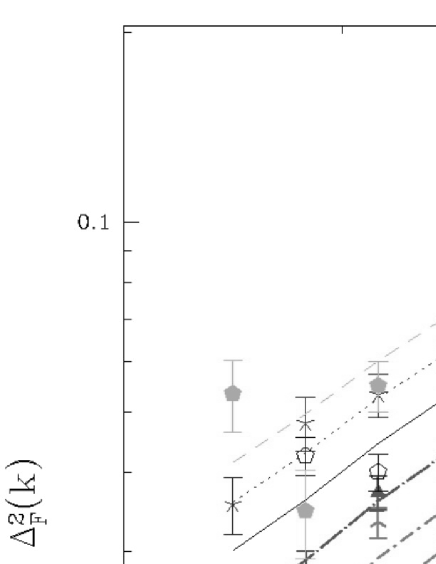
Any measurement of the flux power spectrum and comparison with models also require a careful estimate of the QSO continuum. An optimal method for estimating the QSO continuum in the context of flux power spectra measurements is formulated by Hui et al. (2001). The flux power spectrum was measured from high resolution spectra of 27 QSOs by Kim et al. (2004b, a). The largest and most precise set of measurements by far is that made using a sample of 3035 QSO spectra from the Sloan Digital Sky Survey McDonald et al. (2006). The evolution of the measured flux power spectrum is shown in Figure 18.
Despite their differences, the various approaches have yielded reasonably good agreement on the inferred constraints of cosmological parameters. Using the inversion method, Zaroubi et al. (2006), assuming for the matter power spectrum, obtain . A joint analysis with the WMAP CMB data and a prior on the Hubble constant yields and . Combining the Lyflux power spectrum measurements from the SDSS McDonald et al. (2005b, 2006) with CMB, supernovae and galaxy clustering constraints, Seljak et al. (2006) find the Lyflux power spectrum increases to . They obtain an index of with no evidence for a running spectral index, . In a separate analysis of the measured SDSS flux power spectra, Viel and Haehnelt (2006) obtain , and . Using pure dark matter simulations, Desjacques and Nusser (2005) obtain .
The flux power spectra measurements tend to pull the normalization of the matter power spectrum to larger values compared with estimates based on other methods. This is consistent with the larger values of preferred by cosmological models that match measurements of the pixel flux distribution function and WMAP constraints Meiksin et al. (2001); Meiksin and White (2004). On the other hand, the model comparisons all neglect radiative transfer effects. Allowing for an inverted equation of state over the redshift range , in which underdense regions are warmer than overdense ones, lowers the allowed range for Bolton et al. (2008). There is growing evidence that the equation of state is inverted, or at least not as monotonic as the power spectra and pixel flux distribution analyses have assumed Bolton et al. (2008); Becker et al. (2007). Simulations including radiative transfer show a broad spectrum of temperatures at a given density, including hot underdense regions, in scenarios with late He reionization Tittley and Meiksin (2007).
VII Reionization
VII.1 The epoch of reionization
The reionization of the IGM is one of the principal unsolved problems of cosmological structure formation. Three epochs of reionization of the IGM may be identified, one for hydrogen and two for helium. Because the same radiation sources capable of photoionizing hydrogen would likely also photoionize He to He , only the epochs of hydrogen reionization and full helium reionization to He are likely to be distinct. As discussed in §§ II.2.5 and IV.3.2 above, there is strong evidence full helium reionization occurred at . The most likely He reionization sources are QSOs. The epoch of hydrogen reionization is much less certain. The topic attracted considerable attention following measurements of the IGM Lyoptical depth in high redshift QSOs and CMB measurements of intergalactic Thomson scattering. Unlike full helium reionization, the sources of hydrogen reionization may well be the first sources of radiation to turn on in the Universe, ending the Dark Ages that followed the recombination of the primordial hydrogen and helium plasma. Because of the numerous recent reionization reviews (see § I), I concentrate here only on some of the most salient aspects.
The Lyoptical depth of the IGM measured in the spectra of several QSOs discovered by the Sloan Digital Sky Survey has shown that the IGM was reionized by Fan et al. (2000); Fan et al. (2001a), but the Lyoptical depth rises rapidly towards higher redshifts Becker et al. (2001); Djorgovski et al. (2001); Pentericci et al. (2002); Fan et al. (2004); Fan et al. (2006b); Becker et al. (2007). By , the spectra become so black shortward of Ly, usually only lower limits to the optical depth may be obtained, even using the higher order Lyman resonance transitions. The rapid rise is suggestive of an approach to the EoR. This interpretation is not unique, as only a small neutral fraction is adequate for providing a large Lyoptical depth by Eq. (15). A QSO at moreover shows transmitted flux at White et al. (2003, 2005). Gaps, however, are expected as H regions develop and evolve prior to their complete overlap Furlanetto et al. (2004); Wyithe and Loeb (2006).
The interpretation of the IGM transmission measurements at as evidence for the approach to the EoR is further confounded by WMAP measurements of the intergalactic Thomson optical depth
where is the Thomson cross section, is the comoving electron density (assumed constant and without full helium reionization), and a flat universe is assumed. The 5-year WMAP polarization data yield a marginalized optical depth of Dunkley et al. (2008) up to the EoR, corresponding to an EoR redshift of , assuming reionization was a single, instantaneous event throughout the Universe. The and lower limits are and , respectively Dunkley et al. (2008). These values are lowered slightly to and , allowing for additional astrophysical constraints on the preferred cosmological model from Type Ia supernovae and Baryonic Acoustic Oscillations Hinshaw et al. (2008).
It is worth noting that a non-negligible contribution to the total Thomson optical depth will arise from the IGM prior to the EoR because of the residual electron density frozen out after the Recombination Era. A residual fraction of as little as over the redshift range Page et al. (2007) will produce an additional optical depth of , using Eq. (112). Careful modeling of the contribution to the polarization signal from residual electrons between the Recombination Era and the Epoch of Reionization is required to estimate the contribution due to reionization sources alone.
VII.2 The growth of cosmological H regions
The reionization of the Universe occurs as a consequence of the overlap of H regions driven into the IGM by discrete radiation sources.242424Excepted are scenarios invoking reionization by decaying or annihilating dark matter particles Sciama (1982); Scott et al. (1991); Sciama (1998); Mapelli et al. (2006). Mapelli et al. (2006) find that while some popular dark matter candidates may cause partial reionization, none are able to fully reionize the IGM prior to . Unlike the H region around a star in a galaxy, the growth of cosmological H regions will generally not terminate in a Strömgren sphere, defined as the surface within which the rate of radiative recombinations balances the rate of production of ionizing photons by the source. As the ionization front (I-front) of the H region advances, the expansion of the Universe reduces the density of the gas into which the I-front moves. Unless the I-front encounters a large density inhomogeneity, it will travel unimpeded, lagging further and further behind the Strömgren radius Shapiro (1986), until either the source dies, or the I-front overlaps with another I-front produced by another source or sources.
The advance of the I-front of an isotropic cosmological H region into a multicomponent IGM is described by Shapiro (1986); Shapiro and Giroux (1987); Donahue and Shull (1987); Meiksin and Madau (1993)
| (113) |
where is the proper radius of the I-front, is the mean hydrogen density of the IGM averaged over the various components with volume filling factors , is the Hubble parameter, is the emission rate of ionizing photons from the central sources, is the partial recombination clumping factor of the gas from component , is the number of electrons per hydrogen atom in component (which will contain helium and possibly metals), and is the Case B radiative recombination rate to the level of hydrogen, allowing for ionizations from the ground state by the diffuse radiation emitted following recombinations to the ground state (see § IV.1.1 above). If the diffuse radiation is treated separately, then Case A recombination should be used, and a second set of partial ionization clumping factors must be introduced to represent the volume-averaged product of the local ionization rate and H density in each subcomponent Kohler et al. (2007). If the electron fractions and temperatures of the various components are approximately the same, then may be approximated as and it is convenient to introduce a total recombination clumping factor over all subcomponents, . The recombination term in Eq. (113) is then . (If the diffuse radiation is treated separately, then a similar total ionization clumping factor may be similarly defined.)
Eq. (113) is an approximation for which it is assumed the I-front, within which the gas transforms from neutral to highly ionized, is narrow compared with the radius of the H region. Is also assumes the I-front propagates rapidly compared with the sound speed, so that the effects of gas motion induced by the pressure within the H region may be neglected. It assumes as well that the I-front propagates slowly compared with the speed of light, which formally breaks down in the early stages. Near luminal expansion may be approximately described by replacing on the LHS of Eq. (113) by , where is the RHS of Eq. (113) White et al. (2003); Wyithe and Loeb (2004); Shapiro et al. (2006). This will ensure .
A key uncertainty in the rate at which an H region expands is the recombination clumping factor. Because the clumping factor may be dominated by rare very dense structures, establishing its value from numerical simulations is not straightforward. In particular, systems that produce ionizing photons should be excluded. The dynamical response of clumped structures to an impinging I-front must also be computed, which requires radiative transfer and high spatial resolution. The degree to which a dense cold clump bound by a minihalo impedes the propagation of an I-front in general depends on the mass of the clump and the intensity and spectral shape of the incident radiation field Shapiro et al. (2004); Iliev et al. (2005). A wide range of values for the clumping factor are available in the literature. On the basis of high resolution simulations, Iliev et al. (2007) find the recombination clumping factor is well-fit over the redshift range by
| (114) |
for models using the preferred WMAP 3-year cosmological parameters Spergel et al. (2007).
The evolution in the filling factor of ionized gas as the H regions grow may be quantified by the porosity parameter , which is the product of the volume ionized per source of a given ionizing photon luminosity, integrated over the luminosity function of the sources Donahue and Shull (1987); Meiksin and Madau (1993). For , the IGM becomes completely ionized. Its growth is governed by Madau et al. (1999); Meiksin (2005)
| (115) |
where is the comoving number density of hydrogen, is the production rate of ionizing photons per comoving volume, and is the recombination time at the mean electron density at redshift . If the comoving emissivity of the sources may be approximated as , the ionizing photon production rate is
| (116) |
To solve Eq. (115), it is convenient to define , which is the Hubble time, , measured in units of the recombination time, normalized here at K and including the recombination clumping factor. It is equivalent to the mean number of recombinations per hydrogen atom over a Hubble time. Similar definitions may be introduced for the reionization of He , (assuming all the ionized He is in the form of He ), and of He , . Adopting the clumping factor from Eq. (114) gives nearly constant values for the various over of , , and . For constant , Eq. (115) may be directly integrated, yielding
| (117) | |||||
where is the turn-on redshift of the ionizing sources, and the assumption has been made to obtain the final expression. Similar expressions apply for He and He reionization, on replacing by the appropriate form for He or He , using the production rate of ionizing photons for He or He for , and replacing by . In principle, a recombination clumping factor appropriate to each species must by used since the depth of self-shielding in clumps will differ for different species. To date, simulations have focused on the clumping of ionized hydrogen gas only.
The (comoving) production rate of ionizing photons from the UV background emissivity estimate of Eq. (106) follows from Eq. (116),
| (118) |
where , , and is the spectral index at frequencies above the Lyman edge Meiksin (2005). (This neglects any contribution to the required emissivity from the diffuse recombination radiation from the IGM. If the IGM contributes 30% of the emissivity, should be reduced by the factor 1.3.) Substitution into Eq. (117) and extrapolating Eq. (118) to high redshifts shows that the Universe would be reionized by for , but as late as for . Reionization by , as suggested by observations, requires either a hard spectrum for the sources or an increase over the evolution rate of Eq. (106) in the comoving emissivity at Miralda-Escudé (2003); Meiksin (2005); Bolton and Haehnelt (2007).
VII.3 Sources of reionization
VII.3.1 Galaxies
High redshift star-forming galaxies are generally considered the most likely candidates for the reionization of the Universe. The discovery of high redshift galaxies in deep surveys has sparked much lively debate over whether the population of galaxies that reionized the Universe has now been identified Bouwens et al. (2004); Bunker et al. (2004); Stiavelli et al. (2004); Yan and Windhorst (2004); Bunker et al. (2006); Bouwens et al. (2006). The uncertainties involved preclude any definite decision.
Consider the (comoving) luminosity density at from Bouwens et al. (2006), corrected upward by 50% to allow for internal extinction, of . The conversion rates between (in ), and the production rate of ionizing photons for a Salpeter Initial Mass Function with and and solar metallicity are
| (119) |
Leitherer et al. (1999). For a metallicity of solar, the rates are about 0.1 dex higher for H , 0.2 dex higher for He , and 0.4 dex smaller for He . A similar conversion for H is inferred from Madau et al. (1998) and Madau et al. (1999) for an alternative Salpeter model with and . Assuming that all the ionizing photons escape, applying these rates to the luminosity density at , Eq. (117) (and its variants for He and He reionization, assuming the same recombination clumping factors, which may in fact differ) shows that the galaxies are able to reionize the H by and the He by , while they are unable to reionize the He even by the present epoch. The results for H and He , however, are very sensitive to the uncertainty in the counts and the escape fractions. If only 10% of the ionizing radiation escapes, then the reionization epochs for H and He are reduced dramatically to and 3.7, respectively. Reionization of H by requires , while for He , is needed. Allowing for the upper limits on the counts eases these constraints, as would lower metallicities for the stars Tumlinson and Shull (2000) or an Initial Mass Function heavily tilted to very massive () stars Bromm et al. (2001). On the other hand, a decline in the comoving luminosity density of the sources at would make the case that these sources reionized the Universe less secure. While the population of sources that reionized the Universe may have been discovered in high redshift surveys, a definite conclusion is still premature. There is some evidence for a population of low-luminosity star-forming galaxies at redshifts as high as that may contribute substantially to the total budget of reionizing photons Stark et al. (2007a).
Several semi-analytic estimates for the expected contribution of galaxies to the reionization of both hydrogen and helium have been made Venkatesan et al. (2003); Haiman and Holder (2003); Haiman and Bryan (2006); Shull and Venkatesan (2008). The possible halo masses of the objects that dominate reionization cover a broad range, including systems as small as minihalos with masses and virial temperatures K which would have so far evaded detection. Definitive predictions, however, are hampered by the need to incorporate several poorly determined quantities, including the fraction of baryons in a collapsed halo that are converted into stars, the number of ionizing photons produced by the stars, and the escape fraction of the ionizing radiation from the galaxies. Recent estimates suggest that the efficiency of ionization per galaxy cannot be too high, or a Thomson optical depth would be produced that is too large compared with CMB polarization measurements Haiman and Bryan (2006); Shull and Venkatesan (2008).
VII.3.2 QSOs
The emissivity of QSOs lies well below the requirements for reionization, unless there is a large population of very low luminosity Active Galactic Nuclei (AGN) Meiksin (2005); Srbinovsky and Wyithe (2007); Bolton and Haehnelt (2007). The estimated production rate of ionizing photons from accretion onto massive black holes in the Universe is comparable to the rate from nucleosynthesis in stars Meiksin (2006c): low luminosity AGN may still await discovery at high redshifts. By contrast, QSOs likely fully ionized helium by , and possibly as early as if they have hard spectra extending down to the He photoelectric edge Meiksin (2005).
An interesting alternative class of reionization sources is a possible population of miniquasars, systems produced by intermediate mass black holes with masses growing by accretion onto seed black holes produced by the collapse of very massive Population III stars Madau et al. (2004). Such sources could plausibly reionize the Universe by .
VII.3.3 Other sources
Various alternative sources have been proposed for the reionization of the IGM, including globular star clusters Ricotti (2004), massive Population III stars more generally, with their formation possibly triggered early by primordial magnetic fields Tashiro and Sugiyama (2006), and an early generation of black holes Venkatesan et al. (2001); Ricotti and Ostriker (2004); Ricotti et al. (2005). While these mechanisms are intriguing and have received a variety of theoretical investigations, observational evidence for any of them is as yet wanting. The possibility that sources other than galaxies reionized the IGM, however, should not be discounted: the Universe can surprise.
VII.4 21cm signature of reionization
An altogether novel method for discovering the Epoch of Reionization is through the detection of the 21cm signature from the neutral IGM before and during the reionization process. The emission or absorption of 21cm radiation from a neutral IGM is governed by the spin temperature of the hydrogen, defined by
| (120) |
where and are the singlet and triplet hyperfine levels and K, where is the frequency of the 21cm transition. In the presence of only the CMB radiation, the spin temperature will come into equilibrium with the CMB on a timescale of yr, where is the spontaneous decay rate of the transition. In this case, the spin temperature will be the same as the CMB temperature, and no emission or absorption relative to the CMB will be detectable. A mechanism is needed to decouple the two temperatures. Two mechanisms may couple the spin temperature to the kinetic temperature of the gas. One is the collisions between hydrogen atoms Purcell and Field (1956). The collision-induced coupling between the spin and kinetic temperatures is dominated by spin-exchange between the colliding hydrogen atoms, with possible significant contributions from electron-hydrogen collisions and proton-hydrogen collisions, depending on the ionization fraction and temperature Smith (1966); Dalgarno (1967); Allison and Dalgarno (1969); Zygelman (2005); Furlanetto and Furlanetto (2007); Hirata and Sigurdson (2007). The second, less obvious mechanism, is scattering by Lyphotons Wouthuysen (1952); Field (1958). The Wouthuysen-Field effect mixes the hyperfine levels of neutral hydrogen in its ground state via an intermediate transition to the state. An atom initially in the singlet state may absorb a Lyphoton that puts it in an state, allowing it to return to the triplet state by a spontaneous decay. The combined atomic collision rates are generally too small at the average IGM densities at the redshifts of interest, although collisions may be important in overdense regions, Madau et al. (1997). Instead the dominant mechanism at detectable redshifts for the near future is likely to be Lyscattering.
A patchwork of either 21cm emission, or absorption against the Cosmic Microwave Background, will result Hogan and Rees (1979). Large radio telescopes like LOFAR, the MWA, PAPER, or the SKA offer the prospect of measuring this signature, and so detecting the transitional epoch from a dark universe to one with light. The spin temperature of the neutral hydrogen is
| (121) |
where
| (122) |
are the Lyand collisional pumping efficiencies, respectively. Here is the indirect de-excitation rate of the triplet state via absorption of a Lyphoton to the level, and is assumed. Consideration of the net transition rates between the various hyperfine and levels shows that the transition rate via Lyscattering is related to the total rate
| (123) |
where is the resonance line cross section given by Eq. (12) and is the radiation energy density, by Field (1958). The quantity is the color temperature of the radiation field, given by the harmonic mean of the frequency-specific temperature , weighted by Meiksin (2006b). The factor is the rate of collisional de-excitation of the triplet level. In the absence of collisions, there exists a critical value of which, if greatly exceeded, would drive . This thermalization rate is Madau et al. (1997)
| (124) |
It corresponds to a Lyintensity of , where is a suppression factor of order unity that takes into account the effect of recoils in an expanding medium on the shape of the intensity near the center of the line profile Chen and Miralda-Escudé (2004); Furlanetto et al. (2006). The value of the intensity corresponds to a comparable number of Lyphotons as hydrogen atoms at , and so is comparable to the intensity expected from sources able to reionize the Universe Madau et al. (1997). It is this coincidence that promises that the Wouthuysen-Field mechanism may reveal the IGM prior to its complete reionization.
To illustrate the basic principle of the observations, consider a patch of neutral material with spin temperature , having an angular size on the sky which is large compared with a beamwidth, and radial velocity extent due to the Hubble expansion which is larger than the bandwidth. Following an analysis similar to the derivation of the Gunn-Peterson optical depth (Eq. [15]), and taking into account the reduction of the absorption coefficient due to stimulated emission by the factor for , the intergalactic optical depth at along the line of sight is
| (125) | |||||
which will typically be much less than unity. Here, is the neutral fraction, accounts for fluctuations about the mean hydrogen density, , and a factor of is introduced since only the hydrogen atoms in the singlet state will take part in the absorption. A flat universe is assumed for the second form in Eq. (125) and . Field (1959a) applied Eq. (125) to a search for intergalactic emission or absorption against a background radio galaxy. No clear emission or absorption signature was detected, with an upper limit on the 21cm optical depth of . For , , and , this corresponds to along the line of sight. Adopting and would correspond to an upper limit on the baryon density of assuming the hydrogen was all neutral, showing that early measurements could already have ruled out a baryon-dominated universe closed by a neutral IGM.
In the context of radio measurements of the IGM planned today, an alternative observational strategy consists of cross-correlating measurements of patches separated in either angle or frequency. Possible detections include large isolated H regions, as would be produced by the first QSOS Madau et al. (1997) or, possibly more straightforwardly, a global statistically averaged fluctuation signal from the IGM Tozzi et al. (2000). Foreground contamination, particularly fluctuations in the ionosphere and discrete sources in the Galaxy, pose formidable challenges to detecting the 21cm signature from the Epoch of Reionization. But the development of novel detection strategies suggests the challenges may not be insurmountable. Discussions of the feasibility of the measurements are provided by Wyithe et al. (2005), Bowman et al. (2006), Datta et al. (2007), and in the reviews by Fan et al. (2006a), Furlanetto et al. (2006), and Barkana and Loeb (2007), which also discuss specific reionization scenarios.
VIII The Absorber–Galaxy Connection
Ever since their discovery, intervening absorption systems have held the promise of opening a new window on the evolution of galaxies by probing the gas in galaxies as it was converted into stars, and tracing the feedback of the stars on the gas as supernovae and stellar winds pollute their environment with metals. Despite long and hard searches, direct evidence relating intervening absorbers to galaxies has been scant until only the past few years. Today, the absorber–galaxy connection is fast becoming a boom area in IGM studies.
VIII.1 Galaxy-associated IGM absorption
VIII.1.1 Association of DLAs with galaxies
The motivation for the original systematic Damped LyAbsorber survey was the search for the gaseous disks of galaxies at high redshifts Wolfe et al. (1986). A large number of surveys have been conducted since, summarized in the extensive review by Wolfe et al. (2005). There are several properties of DLAs suggestive of galactic disk material: 1. They are the dominant reservoir of neutral hydrogen at high redshifts () Prochaska et al. (2005); Jorgenson et al. (2006), 2. with the cosmic gas mass density decreasing and metallicity increasing with cosmic time Prochaska et al. (2003). 3. There is evidence for depletion of Fe and Si onto dust grains similar in strength to that in cold gas in the Galaxy Petitjean et al. (2002). 4. There is photometric evidence for reddening by dust, with the amount of extinction increasing with iron column density similar to the trend found for interstellar clouds within the Galaxy Vladilo et al. (2006). 5. Molecular hydrogen is present in about 15–20% of the systems Ledoux et al. (2006b), with the metallicity and depletion factor increasing with the amount of Ledoux et al. (2003). 6. The metallicity of DLAs increases with the velocity width of the line profiles of the low-ionization metals, which presumably trace the gravitational potentials of the systems, and so is suggestive of a mass-metallicity correlation Ledoux et al. (2006a). 7. In addition to a cold low ionization phase, a warm phase is indicated by C and Si absorption systems, and a hot phase is indicated by O absorption detections Fox et al. (2007), demonstrating a complex interstellar medium in DLAs much as is found in disk galaxies. 8. Using a method that deduces the star formation rate from the strength of C as a measure of the amount of gas heating by the photoelectric dust mechanism due to UV heating by massive stars, Wolfe et al. (2003b) infer star formation rates in a presumed cold neutral medium in DLAs similar to that in the interstellar medium of the Galaxy. 9. The inferred global cosmic star formation rate in DLAs at is comparable to that of Lyman Break Galaxies at the same redshift Wolfe et al. (2003a). 10. A search for Lyman Break Galaxies at associated with DLAs shows evidence for a significant spatial correlation between the two, with a cross-correlation length comparable to the autocorrelation length of Lyman Break Galaxies Cooke et al. (2006). 11. Optical counterparts to DLAs at suggest the DLAs arise as part of large (radii of kpc), rotating H disks Chen et al. (2005a). 12. The incidence rate and column density distribution of DLAs at is comparable to those of low redshift galaxies directly measured in H Zwaan et al. (2005).
Despite the circumstantial evidence favoring a galactic disk connection for DLAs, there is strong contrary evidence as well: 1. While they are the dominant reservoir of neutral gas, DLAs contain less than half the mass density of present day stars. 2. The amount of neutral gas in DLAs exceeds the stellar mass in present day disks Wolfe et al. (2005), which suggests they trace the disk component of galaxies, but their metal depletion patterns most often resemble that of warm disk clouds in the Galaxy or halo clouds Ledoux et al. (2002). The difference in the UV metagalactic backgrounds at low and high redshifts may partially account for the apparent discrepancy. 3. The C ∗ inferred star formation rates suggest that a mass in metals should have been produced a factor 30 larger than measured in DLAs Wolfe et al. (2003a). 4. The C ∗ inferred star formation rates somewhat exceed the prediction of the Kennicutt-Schmidt Schmidt (1959); Kennicutt (1998) relation between the star formation rate and gas mass in galaxies Hopkins et al. (2005). Possibly the principal source of heat powering the measured C ∗ cooling rates is star formation in centrally located, compact Lyman Break Galaxies rather than in the bulk of a spatially extended DLA system Wolfe and Chen (2006). 5. DLAs are sufficiently abundant that if they obeyed the Kennicutt-Schmidt relation, then 3% of the sky should be lit up with star-forming DLAs at high redshifts, contrary to observations which find a comoving star formation density a factor 30–100 smaller than predicted Wolfe and Chen (2006). 6. Most puzzling is the rarity of successful follow-up optical identifications. While there is mounting circumstantial evidence that DLAs and Lyman Break Galaxies are associated with the same systems at , only a handful of DLAs show Lyin emission Möller et al. (2004). Galactic counterparts have been confirmed in the optical and near-infrared for about a dozen DLAs at Chen and Lanzetta (2003); Rao et al. (2003); Schulte-Ladbeck et al. (2004); Chen et al. (2005a). The numbers are too few, however, to establish whether or not the galaxies represent a random sampling of the main population of galaxies Wolfe et al. (2005). The nature of DLAs and their relation to present day galaxies remain an enigma.
Simulations set in a CDM cosmology reasonably well reproduce the number of DLAs and their evolution at high redshifts when dissipation due to cooling, star formation and subsequent supernovae feedback and galactic winds are included Nagamine et al. (2004a). The DLAs are found to arise in halos no smaller than those with total masses of about at high redshifts Nagamine et al. (2004a), and almost all in dark matter halos less than Nagamine et al. (2007). Detailed comparisons between the simulated DLAs and observations, however, reveal some discrepancies. The predictions for the number of systems along a line of sight lie somewhat below the measured number. This may be due to overly compact DLAs in the simulations, which also show narrower velocity widths than measured. High resolution simulations with radiative transfer suggest that gas in tidal tails and quasi-filamentary structures also produce DLAs Razoumov et al. (2006), which may help to reconcile the predicted and measured numbers. The star formation rate in the simulations is consistent with the observational estimates in DLAs, however an order of magnitude more metals are produced in the simulations than measured Nagamine et al. (2004b). Simulations with radiative transfer suggest that the UV radiation from stars produced in DLAs and the ambient UV metagalactic background may regulate the rate of star formation within DLAs Iliev et al. (2006). Detailed kinematic comparisons between the simulations and the observations have yet to be made. While the simulations have gone a long way toward accounting for the DLAs within the framework of the CDM model for structure formation, much work still remains to demonstrate that this model correctly describes the origin of most DLAs.
VIII.1.2 Association of metal absorbers with galaxies
Optical and infrared searches for counterparts to metal absorption systems, such as Mg or C , have proven an effective means of discovering galaxies Bergeron and Boissé (1991); Steidel et al. (1994, 1995, 1997); Bouché et al. (2007). On the whole, the galaxies appear to sample the general population of galaxies in the field, although there occur fewer dim blue galaxies in the absorber-selected samples. The morphological and kinematic properties of galaxies associated with Mg systems are reviewed by Churchill et al. (2005).
The spectra of QSOs proximate to galaxies on the sky probe galactic environments. Adelberger et al. (2005) find galaxies at generally show very strong C absorption, , within 40 kpc (proper) of the galaxy, and C absorbers with typical column densities of are found as far out as 80 kpc. The key question is why the metals are near the galaxies. Galaxies are known to be associated with large scale baryonic overdensities, at least as probed by the Lyforest. In the nearby Universe, the stronger absorbers () are spatially correlated with galaxies, although with mixed views over the strength of the cross-correlation compared with the galaxy autocorrelation function Penton et al. (2002); Ryan-Weber (2006); Wilman et al. (2007). At higher redshifts, Adelberger et al. (2005) similarly find galaxies are associated with enhanced amounts of Lyabsorption. If the IGM is polluted by metals, then the proximity of metal absorption systems with galaxies may merely reflect the correlation of H with galaxies. Alternatively, the metals associated with galaxies may have been ejected by the galaxies in a wind following an episode of intense star formation. Either alternative is intriguing. The possibility that galaxies polluted their environment with metals suggests these metals may serve as tracers of the past star formation history of the stars in the galaxy, and so provide independent constraints on their formation. On the other hand, if metal pollution is widespread throughout the IGM, it raises the question of whether the pollution was in situ, produced by some ubiquitous undetected class of stellar systems like a population of high redshift globular star clusters, or are the collective ejecta of galaxies that underwent a superwind phase. In the latter case, it may mean that the evolution of the stellar population of galaxies was not isolated, but that galaxies “talked” with each other as their stars formed, entraining metal enriched material produced by other galaxies. A galactic wind may also delay the onset of star formation in nearby low-mass halos by delivering turbulent kinetic support to the gas Fujita et al. (2004). In extreme cases, a wind may eradicate the gaseous content of nearby low-mass halos through evaporation or shock-driven stripping, suppressing star formation in these systems entirely Scannapieco et al. (2000).
Evidence that high redshift galaxies do impact on the IGM is provided by Adelberger et al. (2005), who find that about a third of the galaxies in their sample at show clearings of weak or absent H absorption out to distances of Mpc (comoving). Simulations suggest, however, that the clearings are consistent with random fluctuations Desjacques et al. (2006); Kawata and Rauch (2007). The kinematic studies of Songaila (2006) show that C systems at with lie in complexes having velocity widths of up to , suggestive of galactic outflows. Lower column density systems lie in complexes with substantially lower velocity widths of , suggesting they are not part of any galactic outflow, although they may be part of residual outflows that were initiated at much higher redshifts Fujita et al. (2004). The evidence for galactic outflows has prompted an increasing interest in the impact of galactic winds on the IGM, discussed next.
VIII.2 Galactic winds and the IGM
Galactic winds occur throughout the Universe, in a variety of environments, over a wide range of galactic masses, including starbursts in the local Universe Heckman et al. (1998) and Lyman Break Galaxies at Pettini et al. (2002) and Lyemitting systems associated with them Wilman et al. (2005). A comprehensive review of galactic winds in the Universe is provided by Veilleux et al. (2005). Reviews specific to the IGM are provided by Aguirre and Schaye (2007) and Bertone et al. (2008).
A natural mechanism for enriching the gas near galaxies with metals is through winds. The possible enrichment by wind ejecta raises further questions: What sort of galaxies ejected the metals? When did they do it? How does the metal pollution relate to the star formation history of the Universe?
Geometric estimates of the impact of galactic winds may be made on the basis of the spatial correlations of the metals and galaxies. Porciani and Madau (2005) find that metal-enriched bubbles of comoving radius kpc expelled at by a biased population of dwarf galaxies with a halo mass of , polluting the region around Lyman Break Galaxies, would account both for the metal abundances measured at and the measured spatial cross-correlation between metals and Lyman Break Galaxies. Using high resolution, high signal-to-noise ratio spectra, Scannapieco et al. (2006b, a) study the clustering properties of high (C and Si ) and low (Mg and Fe ) ionization metal absorption systems. In conjunction with numerical simulations, they find that a uniform distribution of metals fails to reproduce the correlations measured. Modulating the metallicity by the density field similarly fails. They do find, however, that the C correlation function is well-reproduced by assigning the metals to clumps confined to bubbles of comoving radius 2 Mpc around systems with masses exceeding at . A similar model with a slightly larger bubble radius recovers the measured correlations of Mg and Fe at . Both models are degenerate with a biased high-redshift enrichment model with the metals confined to 2.5 Mpc (comoving) radius bubbles around systems at . The results are consistent with two scenarios, metals deposited by winds from massive galaxies at , or by winds from dwarf galaxies at high redshifts, . An early wind model is also favored by the near constant mass density associated with C systems over the broad redshift range Songaila (2005); Ryan-Weber et al. (2006). Whether any of these scenarios are viable depends on whether wind models that support them may be physically realized.
Correlations between low redshift absorption systems and galaxies provide a potentially powerful means of inferring the origins of the metals. Tumlinson and Fang (2005) find that dwarf galaxies are able to reproduce the line-of-sight number density of O systems if they produce winds extending out to about 200 kpc, while luminous galaxies would need to produce winds extending to Mpc. Similar results are obtained from the O survey analysis of Stocke et al. (2006a), who match O systems at with galaxies in the field. They find the metal systems have median distances of 350–500 kpc (for ) from galaxies, and 200–270 kpc around galaxies. A contribution from galaxies is required to reproduce the line-of-sight number density of O absorbers.
While these results are consistent with the ejection of metals from the galaxies detected, this is not the only possible picture. The metals may have arisen at earlier times in smaller systems that eventually merged into the galaxies seen. Alternatively, they may have been ejected from much smaller systems, perhaps as small as globular star clusters or very faint dwarf galaxies, that are spatially correlated with the visible galaxies. The metals may also have been deposited very early in the history of the Universe, perhaps by blowout from the projenitors of present day galaxies in superwinds or possibly driven out by the impact of AGN that may have been active in the projenitors.
As a galactic wind expands into the IGM, it will drive a shockfront that sweeps up the surrounding gas into a thin shell just behind the shock. In this limit, the thin-shell approximation may be made to describe the advance of the shockfront. Denoting the distance of the shockfront from the center of the galaxy by , the mass of the expanding gas interior to by , the mean interior pressure by and enthalpy density by , the external pressure and density by and , respectively, the velocity of the external gas relative to the galaxy by , the gravitational potential energy of the wind gas by , and assuming mass injection from the center at the rate with velocity , the equations describing the evolution of the shockfront radius and the interior thermal energy of the bubble powered by energy injected at the rate and cooling at the rate are, in the thin-shell approximation Ostriker and McKee (1988); Madau et al. (2001),
| (126) | |||||
| (127) | |||||
where isothermal jump conditions across the shock front have been assumed for the energy equation, presuming the wind expands into a photoionized medium. A clumpy interior is allowed for due to the presence of clouds with a volume filling factor and spatial density and cross section corresponding to a mean free path , which enters as a drag term on the advance of the shockfront in Eq. (126). The interior net cooling will be dominated by Compton cooling at high redshifts and two body atomic processes, which in turn depend on the gas clumping factor, and radiative heating from the galaxy or UV metagalactic background at lower redshifts. The second and fourth terms on the RHS of Eq. (127) account for energy loss due to work done by the shock on the surrounding gas and on crushing interior clouds, respectively.
The factors in Eqs. (126)-(127) highlight the various uncertainties in any galactic wind calculation. The rate of mass and energy injection by the stars and supernovae depend on the rate of star formation and the Initial Mass Function of the stars, which may have a lower upper mass cutoff in starbursts compared with normal galaxies Leitherer and Heckman (1995), or may be dominated by massive stars if the metallicity is low Bromm and Loeb (2003). The cooling rate will depend on the metallicity of the bubble interior, its clumpiness, and on how well mixed the metals are. It will also depend on the temperature of the interior gas, which requires a specification of the amount of interior mass even though it is negligible compared with the mass in the shell. Most of the interior mass results from evaporative losses from the contact surface between the hot interior and the cool shell Madau et al. (2001). The rate of evaporation depends on the degree to which thermal heat conduction may be suppressed by interior magnetic fields, although mechanical heat input balancing adiabatic expansion losses dominates the interior thermodynamics, so this may not be critical. The strength of the shock front may be substantially dissipated as the shock overtakes small clouds and crushes them. Lastly, the progress of the shockfront depends on the environment of the galaxy, which will differ in different directions, so that the winds will in general be anisotropic. The acceleration of dense gas by hot rarefied gas and the motion of surfaces past one another as the bubble penetrates the IGM will also generally be subject to Rayleigh-Taylor and Kelvin-Helmholtz instabilities, giving rise to the mixing of gas components with vastly contrasting densities and temperatures and the formation of eddies both at the surface of the bubble and in its interior as the shell fragments. Thermal instabilities may also play a role. Magnetic fields will generally also affect the fragmentation of the expanding shell, and may affect the crushing of interior clouds. No numerical simulation is able to contend with all these factors: the required spatial resolution, range in timescales, and number of physical processes involved are far too demanding. Instead, simulators must resort to the art of approximation.
Several estimates of the possible impact of galactic winds on the IGM have been made. An instantaneous stellar burst of , typical of a dwarf galaxy with total halo mass and allowing for a conversion efficiency of gas mass into stars, produces a mechanical luminosity provided by supernovae and stellar winds of W Leitherer et al. (1999), assuming a Salpeter Initial Mass Function between . The contribution of supernovae dies off after about yr, and the mechanical luminosity plummets, having yielded a total mechanical energy input of J. If the wind is allowed to expand until it reaches pressure equilibrium with the surrounding IGM, then a maximum distance the wind travels may be estimated. For example, if a fraction of the mechanical energy is available to power the wind (taking into account losses internal to the galaxy and as the wind expands), balancing the mean internal pressure (assuming for the ionized interior gas), where is the bubble volume, with the pressure of the external IGM , gives a maximum comoving bubble radius of kpc.
The maximum radius is comparable to the geometric estimates discussed above. Taking account of radiative losses, however, stalls the expansion before it reaches the maximum value Madau et al. (2001). More massive galaxies driving stronger winds might be appealed to, but this is problematic on two grounds: they are much rarer than dwarf galaxies at high redshifts and the ram pressure of the surrounding infalling IGM can smother the expansion of the wind Fujita et al. (2004).
An estimate of the maximum mass halo able to produce an escaping wind may be made as follows. Galaxies have nearly flat rotation curves, corresponding to envelope density profiles slightly steeper than Peebles (1993). The infall velocity of the gas is then , where is the mass of the virialized halo of mean density and radius (§ V.2). Assuming the gaseous component follows the profile of the envelope of dark matter, the ram pressure at the surface of the bubble is for . If the ram pressure dominates the IGM pressure, then it will determine the stalling radius where it matches , according to Eq. (126). The criterion (for ) imposes the upper limit on the virial mass of the galaxies able to produce escaping winds of
| (128) |
in good agreement with hydrodynamical computations Fujita et al. (2004). For a more complete treatment, hydrodynamical simulations are required. Examples of recent wind simulations include Theuns et al. (2002b), Aguirre et al. (2005), Cen et al. (2005), Cen and Ostriker (2006), Oppenheimer and Davé (2006), Kobayashi et al. (2007), and Kawata and Rauch (2007).
IX Prospects for the Future
The future of IGM studies is entering a new phase in both observations and computations that promises to settle a number of outstanding questions. Prominent among these are the circumstances that led to the reionization of the Universe. At the same time, the growing recognition of the relationship between the IGM and galaxies is likely to shift the subject increasingly toward a merger with the more embracing subject of galaxy formation. Perhaps most spectacularly, imminent and planned detectors and space missions may open up a new era in IGM science: direct imaging of the structure of the IGM in the infrared and radio.
Recent years have witnessed the detection of high redshift Lyemitting galaxies, long-sought as candidates for the first forming galaxies Partridge and Peebles (1967). Measurements of the Lyemitter luminosity function and its evolution would in principle provide evidence for the reionization epoch, as the Ly radiative damping edge of neutral patches would increasingly erode the lines and produce a sharp decrease in the luminosity function. Evidence for such rapid evolution over the redshift range has been obtained from the Subaru Deep Field Kashikawa et al. (2006); Iye et al. (2006). The interpretation of any decline, however, is complicated by systematics, such as the unknown evolution in the dust content, the structure of the local IGM that may produce a Ly radiative damping wing, and the mass of the systems producing star formation, as well as the possible infall of the IGM towards the source and the impact of winds produced by the source on the surrounding IGM, all of which could affect the intensity and shape of the Lyemission line and so the evolution of the Lyluminosity function Santos (2004); Haiman and Cen (2005); Nilsson et al. (2007); Davé et al. (2006). McQuinn et al. (2007) suggest these uncertainties may be circumvented by using the angular correlation function of the Lyemitters. The angular correlations will be strongly modulated by H regions during the EoR on large scales where the dark matter fluctuations are weak, providing a distinctive signature of reionization. Much improved Lyemitter statistics are anticipated with current or upcoming narrow band surveys which may make it possible to realize these tests Horton et al. (2004); Gardner et al. (2006); Ouchi et al. (2008); Stark et al. (2007b).
Anticipated CMB polarization measurements are expected to further narrow the redshift range during which reionization occurred. Polarization anisotropy measurements on arcminute scales by the Planck satellite,252525http://www.rssd.esa.int/Planck to be launched in 2008, may reveal the expected patchiness of reionization, which may be used to discriminate between competing reionization scenarios Santos et al. (2003); Zahn et al. (2005); McQuinn et al. (2005). The Atacama Cosmology Telescope (ACT)262626http://www.physics.princeton.edu/act/ and the South Pole Telescope (SPT)272727http://spt.uchicago.edu/ have already embarked on such measurements.
The relationship between the IGM and galaxies will be further clarified by upcoming galaxy surveys, especially at low redshifts. UV spectroscopy with the Cosmic Origins Spectrograph (COS),282828http://cos.colorado.edu to be installed on HST in 2008, will refine the measurements of low to moderate redshift metal absorption systems, and increase sample sizes by an order of magnitude, greatly improving the statistics on the correlations with galaxies. Currently detections of the WHIM have been confined almost entirely to O measurements. Detections of further high ionization species would be possible using COS as well as the spectroscopic capabilities of the proposed x-ray satellite Constellation-X or a possible smaller scale satellite with high resolution x-ray spectroscopic capability Nicastro (2006), providing important diagnostics of the physical properties of the WHIM. LOFAR is expected to detect the synchrotron emission from starburst galaxies, which with follow-up optical, UV and sub-millimeter observations, will provide a wealth of data that may establish the impact of winds on the IGM over a wide range of redshifts, including the spreading of metals. Even greater numbers may be detected by a Square Kilometer Array, with an expected detection rate of several thousand at per square degree surveyed. Optical spectroscopy using a Giant Segmented Mirror Telescope (GSMT),292929http://www.gsmt.noao.edu such as the Thirty Meter Telescope (TMT)303030http://www.tmt.sorg and the Giant Magellan Telescope (GMT),313131http://www.gmto.org and an Extremely Large Telescope (ELT)323232http://www.eso.org/projects/e-elt/ could measure the temperature of the moderate and even low density components of the IGM by measuring the velocity widths of multiple metal line absorption systems. Deep photometric surveys with such very large telescopes could detect very low luminosity galaxies that may be associated with low redshift metal absorption systems. The Ultra Deep Survey of the James Webb Space Telescope, 333333http://www.jwst.nasa.gov/ to be launched in 2013, will detect dwarf galaxies out to redshifts of , and so may positively identify the population of galaxies which reionized the IGM Gardner et al. (2006); Windhorst et al. (2006). These multiband measurements, extending from the radio through x-rays, will help to establish the metal pollution patterns throughout the IGM and their relationship with star-forming galaxies.
These advances will enable simulations to provide a complete description of the evolution of the IGM. Such a prospect would open up new opportunities for other areas of astrophysics and cosmology to exploit the IGM as a tool for testing models of interest. For example, the abundances and distribution of metals as well as the line widths of metal and hydrogen absorption features around galaxies could place stringent constraints on galaxy formation models and the winds young galaxies may produce, including the possible impact on the host galaxy and its surroundings of an embedded AGN Sijacki et al. (2007). The imaging of the IGM around QSO sources could directly reveal the opening angles of their emission cones and relative orientation to the observer, placing strong constraints on unification models of AGN.
Precise predictions for the absorption statistics of the IGM may provide valuable constraints on modifications of standard cosmological models such as those allowing for a “dark energy” equation of state. Dark energy will affect the growth rate of structures in the IGM, possibly at a detectable level in future surveys Viel et al. (2003b). The density fluctuations in the IGM along the line of sight and transvere directions will differ as a consequence of the difference between radial and angular distances at high redshifts Alcock and Paczynski (1979). With sufficient statistics, the difference may be detectable in the correlation function or power spectrum measurements of the transmitted Ly flux through the IGM Hui et al. (1999); McDonald and Miralda-Escudé (1999); Marble et al. (2008a, b). Even more ambitious would be the direct detection of the expansion of the Universe through the monitoring of absorption lines along fixed lines of sight over a period of several years through spectroscopy on extremely large telescopes Corasaniti et al. (2007); Liske et al. (2008). Since realizing such a measurement would require the development of an extraordinarily stable detection system and adequate taming of systematics associated with variations in the QSO brightness and spectral shape and their effects on the noise statistics, such a project may spur efforts to investigate the technical characteristics of large telescopes and the behavior of QSOs at unprecedented levels of accuracy.
The next few years may produce the first images of the IGM. Ionizing radiation reprocessed by the neutral gas in Lyman Limit Systems into Lyphotons may soon be detectable by upcoming Lynarrow-band detectors Hogan and Weymann (1987); Gould and Weinberg (1996); Cantalupo et al. (2005, 2007). It my even be possible to detect the Lyphotons emitted by a central source like a QSO and scattered by the surrounding neutral IGM prior to reionization Loeb and Rybicki (1999) or Lyphotons produced by collisional excitation within the rapidly expanding ionization fronts during the EoR Cantalupo et al. (2008), providing Lytomographic imaging of the neutral IGM. Such detections would complement the planned IGM imaging by the LOFAR, MWA and SKA radio facilities using 21cm tomography. Cross-correlations between the Lyand radio images may help to establish statistically significant detections.
At even higher redshifts, 21cm tomography prior to reionization may become possible through the production of a 21cm signature via Lyand collisional decoupling of the spin temperature from the CMB. At , collisional decoupling alone is adequate, offering the opportunity to explore the redshift desert and examine the primordial density fluctuation power spectrum on scales smaller than may be reached by CMB measurements. Such measurements could probe the structure of an inflationary potential and induced non-gaussian fluctuations Loeb and Zaldarriaga (2004); Bharadwaj and Ali (2004); Barkana and Loeb (2005); McQuinn et al. (2006); Pillepich et al. (2007). Astrophysical and instrumental systematics and sources of radio frequency interference (RFI), both man made and natural, such as arises from the ionosphere, likely preclude such measurements using currently planned radio facilities Bowman et al. (2007). These limitations, however, may be circumvented by placing a radio telescope in space. Even more adventurous would be to build a much larger facility on the far side of the Moon, where it would be shielded from terrestrial RFI Carilli et al. (2007). The exploration of long wavelengths unavailable to terrestrial radio astronomy would open up a new panorama on the Universe, introducing a new era of “Astronomy on the Far Side.” While not all of these prospects may materialize, others not currently envisaged will surely arise, ensuring that IGM science will continue to flourish for many years to come.
Acknowledgments
This review benefitted from discussions with and comments by J. Bland-Hawthorne, J. Bolton, A. Ferrara, J. Higgins, P. Madau, J. Peterson, M. Rauch, S. Reynolds, J. Schaye, E. Tittley, D. Turnshek and M. White.
References
- Abel et al. (1997) Abel, T., P. Anninos, Y. Zhang, and M. L. Norman, 1997, New Astronomy 2, 181.
- Abel and Haehnelt (1999) Abel, T., and M. G. Haehnelt, 1999, Astrophys. J. 520, L13.
- Adelberger et al. (2005) Adelberger, K. L., A. E. Shapley, C. C. Steidel, M. Pettini, D. K. Erb, and N. A. Reddy, 2005, Astrophys. J. 629, 636.
- Agafonova et al. (2005) Agafonova, I. I., M. Centurión, S. A. Levshakov, and P. Molaro, 2005, Astron. Astrophys. 441, 9.
- Agafonova et al. (2007) Agafonova, I. I., S. A. Levshakov, D. Reimers, C. Fechner, D. Tytler, R. A. Simcoe, and A. Songaila, 2007, Astron. Astrophys. 461, 893.
- Aguirre and Schaye (2007) Aguirre, A., and J. Schaye, 2007, in EAS Publications Series, volume 24 of Engineering and Science, pp. 165–175.
- Aguirre et al. (2005) Aguirre, A., J. Schaye, L. Hernquist, S. Kay, V. Springel, and T. Theuns, 2005, Astrophys. J. 620, L13.
- Aguirre et al. (2004) Aguirre, A., J. Schaye, T.-S. Kim, T. Theuns, M. Rauch, and W. L. W. Sargent, 2004, Astrophys. J. 602, 38.
- Akerman et al. (2005) Akerman, C. J., S. L. Ellison, M. Pettini, and C. C. Steidel, 2005, Astron. Astrophys. 440, 499.
- Alcock and Paczynski (1979) Alcock, C., and B. Paczynski, 1979, Nature (London) 281, 358.
- Aldcroft et al. (1993) Aldcroft, T. L., M. Elvis, and J. Bechtold, 1993, Astron. J. 105, 2054.
- Aldrovandi and Pequignot (1973) Aldrovandi, S. M. V., and D. Pequignot, 1973, Astron. Astrophys. 25, 137.
- Allende Prieto et al. (2001) Allende Prieto, C., D. L. Lambert, and M. Asplund, 2001, Astrophys. J. 556, L63.
- Allende Prieto et al. (2002) Allende Prieto, C., D. L. Lambert, and M. Asplund, 2002, Astrophys. J. 573, L137.
- Allison and Dalgarno (1969) Allison, A. C., and A. Dalgarno, 1969, Astrophys. J. 158, 423.
- Anderson et al. (1999) Anderson, S. F., C. J. Hogan, B. F. Williams, and R. F. Carswell, 1999, Astron. J. 117, 56.
- Aracil et al. (2004) Aracil, B., P. Petitjean, C. Pichon, and J. Bergeron, 2004, Astron. Astrophys. 419, 811.
- Arnaud and Rothenflug (1985) Arnaud, M., and R. Rothenflug, 1985, Astron. Astrophys. Suppl. Ser. 60, 425.
- Arons and McCray (1969) Arons, J., and R. McCray, 1969, Astrophys. J. 158, L91+.
- Arons and McCray (1970a) Arons, J., and R. McCray, 1970a, Astrophys. J. Lett. 5, 287.
- Arons and McCray (1970b) Arons, J., and R. McCray, 1970b, Astrophys. J. Lett. 5, 123.
- Asplund (2003) Asplund, M., 2003, ArXiv Astrophysics e-prints eprint astro-ph/0302409.
- Atwood et al. (1985) Atwood, B., J. A. Baldwin, and R. F. Carswell, 1985, Astrophys. J. 292, 58.
- Bahcall et al. (1968) Bahcall, J. N., J. L. Greenstein, and W. L. W. Sargent, 1968, Astrophys. J. 153, 689.
- Bahcall and Salpeter (1965) Bahcall, J. N., and E. E. Salpeter, 1965, Astrophys. J. 142, 1677.
- Bahcall et al. (1967) Bahcall, J. N., W. L. W. Sargent, and M. Schmidt, 1967, Astrophys. J. 149, L11+.
- Bahcall and Spitzer (1969) Bahcall, J. N., and L. J. Spitzer, 1969, Astrophys. J. 156, L63+.
- Bahcall and Wolf (1968) Bahcall, J. N., and R. A. Wolf, 1968, Astrophys. J. 152, 701.
- Bajtlik et al. (1988) Bajtlik, S., R. C. Duncan, and J. P. Ostriker, 1988, Astrophys. J. 327, 570.
- Barkana and Loeb (2005) Barkana, R., and A. Loeb, 2005, Astrophys. J. 624, L65.
- Barkana and Loeb (2007) Barkana, R., and A. Loeb, 2007, Reports of Progress in Physics 70, 627.
- Barlow and Tytler (1998) Barlow, T. A., and D. Tytler, 1998, Astron. J. 115, 1725.
- Baron et al. (1989) Baron, E., R. F. Carswell, C. J. Hogan, and R. J. Weymann, 1989, Astrophys. J. 337, 609.
- Bechtold (1994) Bechtold, J., 1994, Astrophys. J. Suppl. Ser. 91, 1.
- Bechtold (2003) Bechtold, J., 2003, in Galaxies at High Redshift, edited by I. Pérez-Fournon, M. Balcells, F. Moreno-Insertis, and F. Sánchez, pp. 131–184.
- Bechtold et al. (1994) Bechtold, J., A. P. S. Crotts, R. C. Duncan, and Y. Fang, 1994, Astrophys. J. 437, L83.
- Bechtold et al. (2002) Bechtold, J., A. Dobrzycki, B. Wilden, M. Morita, J. Scott, D. Dobrzycka, K.-V. Tran, and T. L. Aldcroft, 2002, Astrophys. J. Suppl. Ser. 140, 143.
- Bechtold et al. (1987) Bechtold, J., R. J. Weymann, Z. Lin, and M. A. Malkan, 1987, Astrophys. J. 315, 180.
- Becker et al. (2007) Becker, G. D., M. Rauch, and W. L. W. Sargent, 2007, Astrophys. J. 662, 72.
- Becker et al. (2004) Becker, G. D., W. L. W. Sargent, and M. Rauch, 2004, Astrophys. J. 613, 61.
- Becker et al. (2001) Becker, R. H., X. Fan, R. L. White, M. A. Strauss, V. K. Narayanan, R. H. Lupton, J. E. Gunn, J. Annis, N. A. Bahcall, J. Brinkmann, A. J. Connolly, I. Csabai, et al., 2001, Astron. J. 122, 2850.
- Bergeron and Boissé (1991) Bergeron, J., and P. Boissé, 1991, Astron. Astrophys. 243, 344.
- Bergeron et al. (1994) Bergeron, J., P. Petitjean, W. L. W. Sargent, J. N. Bahcall, A. Boksenberg, G. F. Hartig, B. T. Jannuzi, S. Kirhakos, B. D. Savage, D. P. Schneider, D. A. Turnshek, R. J. Weymann, et al., 1994, Astrophys. J. 436, 33.
- Bergeron and Stasinska (1986) Bergeron, J., and G. Stasinska, 1986, Astron. Astrophys. 169, 1.
- Bergvall et al. (2006) Bergvall, N., E. Zackrisson, B.-G. Andersson, D. Arnberg, J. Masegosa, and G. Östlin, 2006, Astron. Astrophys. 448, 513.
- Bernardi et al. (2003) Bernardi, M., R. K. Sheth, M. SubbaRao, G. T. Richards, S. Burles, A. J. Connolly, J. Frieman, R. Nichol, J. Schaye, D. P. Schneider, D. E. Vanden Berk, D. G. York, et al., 2003, Astron. J. 125, 32.
- Bertone et al. (2008) Bertone, S., J. Schaye, and K. Dolag, 2008, Space Science Reviews 134, 295.
- Bertschinger (1998) Bertschinger, E., 1998, Annu. Rev. Astron. Astrophys. 36, 599.
- Bharadwaj and Ali (2004) Bharadwaj, S., and S. S. Ali, 2004, Mon. Not. R. Astron. Soc. 352, 142.
- Bi (1993) Bi, H., 1993, Astrophys. J. 405, 479.
- Bi and Davidsen (1997) Bi, H., and A. F. Davidsen, 1997, Astrophys. J. 479, 523.
- Bi et al. (1992) Bi, H. G., G. Boerner, and Y. Chu, 1992, Astron. Astrophys. 266, 1.
- Black (1981) Black, J. H., 1981, Mon. Not. R. Astron. Soc. 197, 553.
- Blumenthal (1974) Blumenthal, G. R., 1974, Astrophys. J. 188, 121.
- Boisse et al. (1992) Boisse, P., O. Boulade, D. Kunth, D. Tytler, and L. Vigroux, 1992, Astron. Astrophys. 262, 401.
- Boksenberg (1972) Boksenberg, A., 1972, in Proceedings of ESO/CERN conference on auxiliary instrumentation for large telescopes, p. 295 - 316, edited by S. Laustsen and A. Reiz, pp. 295–316.
- Bolton et al. (2004) Bolton, J., A. Meiksin, and M. White, 2004, Mon. Not. R. Astron. Soc. 348, L43.
- Bolton and Haehnelt (2007) Bolton, J. S., and M. G. Haehnelt, 2007, Mon. Not. R. Astron. Soc. 382, 325.
- Bolton et al. (2006) Bolton, J. S., M. G. Haehnelt, M. Viel, and R. F. Carswell, 2006, Mon. Not. R. Astron. Soc. 366, 1378.
- Bolton et al. (2005) Bolton, J. S., M. G. Haehnelt, M. Viel, and V. Springel, 2005, Mon. Not. R. Astron. Soc. 357, 1178.
- Bolton et al. (2008) Bolton, J. S., M. Viel, T.-S. Kim, M. G. Haehnelt, and R. F. Carswell, 2008, Mon. Not. R. Astron. Soc. 386, 1131.
- Bond et al. (1996) Bond, J. R., L. Kofman, and D. Pogosyan, 1996, Nature (London) 380, 603.
- Bond et al. (1988) Bond, J. R., A. S. Szalay, and J. Silk, 1988, Astrophys. J. 324, 627.
- Boroson and Green (1992) Boroson, T. A., and R. F. Green, 1992, Astrophys. J. Suppl. Ser. 80, 109.
- Bouché et al. (2007) Bouché, N., M. T. Murphy, C. Péroux, R. Davies, F. Eisenhauer, N. M. Förster Schreiber, and L. Tacconi, 2007, Astrophys. J. 669, L5.
- Bouwens et al. (2006) Bouwens, R. J., G. D. Illingworth, J. P. Blakeslee, and M. Franx, 2006, Astrophys. J. 653, 53.
- Bouwens et al. (2004) Bouwens, R. J., R. I. Thompson, G. D. Illingworth, M. Franx, P. G. van Dokkum, X. Fan, M. E. Dickinson, D. J. Eisenstein, and M. J. Rieke, 2004, Astrophys. J. 616, L79.
- Bowman et al. (2006) Bowman, J. D., M. F. Morales, and J. N. Hewitt, 2006, Astrophys. J. 638, 20.
- Bowman et al. (2007) Bowman, J. D., M. F. Morales, and J. N. Hewitt, 2007, Astrophys. J. 661, 1.
- Boyle et al. (1988) Boyle, B. J., T. Shanks, and B. A. Peterson, 1988, Mon. Not. R. Astron. Soc. 235, 935.
- Briggs et al. (1989) Briggs, F. H., A. M. Wolfe, H. S. Liszt, M. M. Davis, and K. L. Turner, 1989, Astrophys. J. 341, 650.
- Bromm et al. (2001) Bromm, V., R. P. Kudritzki, and A. Loeb, 2001, Astrophys. J. 552, 464.
- Bromm and Loeb (2003) Bromm, V., and A. Loeb, 2003, Nature (London) 425, 812.
- Bruzual and Charlot (2003) Bruzual, G., and S. Charlot, 2003, Mon. Not. R. Astron. Soc. 344, 1000.
- Bryan et al. (1999) Bryan, G. L., M. Machacek, P. Anninos, and M. L. Norman, 1999, Astrophys. J. 517, 13.
- Bryan and Machacek (2000) Bryan, G. L., and M. E. Machacek, 2000, Astrophys. J. 534, 57.
- Bunker et al. (2006) Bunker, A., E. Stanway, R. Ellis, R. McMahon, L. Eyles, and M. Lacy, 2006, New Astronomy Review 50, 94.
- Bunker et al. (2004) Bunker, A. J., E. R. Stanway, R. S. Ellis, and R. G. McMahon, 2004, Mon. Not. R. Astron. Soc. 355, 374.
- Burles and Tytler (1996) Burles, S., and D. Tytler, 1996, Astrophys. J. 460, 584.
- Burles and Tytler (1998a) Burles, S., and D. Tytler, 1998a, Astrophys. J. 499, 699.
- Burles and Tytler (1998b) Burles, S., and D. Tytler, 1998b, Astrophys. J. 507, 732.
- Burles and Tytler (2002) Burles, S., and D. Tytler, 2002, Astrophys. J. 573, 471.
- Cantalupo et al. (2007) Cantalupo, S., S. J. Lilly, and C. Porciani, 2007, Astrophys. J. 657, 135.
- Cantalupo et al. (2008) Cantalupo, S., C. Porciani, and S. J. Lilly, 2008, Astrophys. J. 672, 48.
- Cantalupo et al. (2005) Cantalupo, S., C. Porciani, S. J. Lilly, and F. Miniati, 2005, Astrophys. J. 628, 61.
- Carilli et al. (2007) Carilli, C. L., J. N. Hewitt, and A. Loeb, 2007, ArXiv Astrophysics e-prints eprint astro-ph/0702070.
- Carswell et al. (1991) Carswell, R. F., K. M. Lanzetta, H. C. Parnell, and J. K. Webb, 1991, Astrophys. J. 371, 36.
- Carswell et al. (1987) Carswell, R. F., J. K. Webb, J. A. Baldwin, and B. Atwood, 1987, Astrophys. J. 319, 709.
- Casey et al. (2008) Casey, C. M., C. D. Impey, C. E. Petry, A. R. Marble, and R. Davé, 2008, Astron. J. 136, 181.
- Cen et al. (1994) Cen, R., J. Miralda-Escudé, J. P. Ostriker, and M. Rauch, 1994, Astrophys. J. 437, L9.
- Cen et al. (2005) Cen, R., K. Nagamine, and J. P. Ostriker, 2005, Astrophys. J. 635, 86.
- Cen and Ostriker (1999) Cen, R., and J. P. Ostriker, 1999, Astrophys. J. 514, 1.
- Cen and Ostriker (2006) Cen, R., and J. P. Ostriker, 2006, Astrophys. J. 650, 560.
- Chand et al. (2004) Chand, H., R. Srianand, P. Petitjean, and B. Aracil, 2004, Astron. Astrophys. 417, 853.
- Charlton et al. (1993) Charlton, J. C., E. E. Salpeter, and C. J. Hogan, 1993, Astrophys. J. 402, 493.
- Charlton et al. (1994) Charlton, J. C., E. E. Salpeter, and S. M. Linder, 1994, Astrophys. J. 430, L29.
- Chen et al. (2005a) Chen, H.-W., R. C. Kennicutt, Jr., and M. Rauch, 2005a, Astrophys. J. 620, 703.
- Chen and Lanzetta (2003) Chen, H.-W., and K. M. Lanzetta, 2003, Astrophys. J. 597, 706.
- Chen et al. (2005b) Chen, H.-W., J. X. Prochaska, B. J. Weiner, J. S. Mulchaey, and G. M. Williger, 2005b, Astrophys. J. 629, L25.
- Chen and Miralda-Escudé (2004) Chen, X., and J. Miralda-Escudé, 2004, Astrophys. J. 602, 1.
- Chen et al. (2003) Chen, X., D. H. Weinberg, N. Katz, and R. Davé, 2003, Astrophys. J. 594, 42.
- Churchill et al. (2005) Churchill, C., C. Steidel, and G. Kacprzak, 2005, in Extra-Planar Gas, edited by R. Braun, volume 331 of Astronomical Society of the Pacific Conference Series, pp. 387–+.
- Churchill et al. (1999) Churchill, C. W., J. R. Rigby, J. C. Charlton, and S. S. Vogt, 1999, Astrophys. J. Suppl. Ser. 120, 51.
- Ciardi et al. (2002) Ciardi, B., S. Bianchi, and A. Ferrara, 2002, Mon. Not. R. Astron. Soc. 331, 463.
- Clarke and Oey (2002) Clarke, C., and M. S. Oey, 2002, Mon. Not. R. Astron. Soc. 337, 1299.
- Colbert and Malkan (2002) Colbert, J. W., and M. A. Malkan, 2002, Astrophys. J. 566, 51.
- Cooke et al. (2006) Cooke, J., A. M. Wolfe, E. Gawiser, and J. X. Prochaska, 2006, Astrophys. J. 652, 994.
- Cooke et al. (2005) Cooke, J., A. M. Wolfe, J. X. Prochaska, and E. Gawiser, 2005, Astrophys. J. 621, 596.
- Corasaniti et al. (2007) Corasaniti, P.-S., D. Huterer, and A. Melchiorri, 2007, Phys. Rev. D 75(6), 062001.
- Cowie and Songaila (1998) Cowie, L. L., and A. Songaila, 1998, Nature (London) 394, 44.
- Cowie et al. (1995) Cowie, L. L., A. Songaila, T.-S. Kim, and E. M. Hu, 1995, Astron. J. 109, 1522.
- Crighton et al. (2004) Crighton, N. H. M., J. K. Webb, A. Ortiz-Gil, and A. Fernández-Soto, 2004, Mon. Not. R. Astron. Soc. 355, 1042.
- Cristiani et al. (1995) Cristiani, S., S. D’Odorico, A. Fontana, E. Giallongo, and S. Savaglio, 1995, Mon. Not. R. Astron. Soc. 273, 1016.
- Croft (2004) Croft, R. A. C., 2004, Astrophys. J. 610, 642.
- Croft et al. (2002a) Croft, R. A. C., L. Hernquist, V. Springel, M. Westover, and M. White, 2002a, Astrophys. J. 580, 634.
- Croft et al. (2002b) Croft, R. A. C., D. H. Weinberg, M. Bolte, S. Burles, L. Hernquist, N. Katz, D. Kirkman, and D. Tytler, 2002b, Astrophys. J. 581, 20.
- Croft et al. (1997) Croft, R. A. C., D. H. Weinberg, N. Katz, and L. Hernquist, 1997, Astrophys. J. 488, 532.
- Croft et al. (1998) Croft, R. A. C., D. H. Weinberg, N. Katz, and L. Hernquist, 1998, Astrophys. J. 495, 44.
- Croft et al. (1999) Croft, R. A. C., D. H. Weinberg, M. Pettini, L. Hernquist, and N. Katz, 1999, Astrophys. J. 520, 1.
- Croom et al. (2004) Croom, S. M., R. J. Smith, B. J. Boyle, T. Shanks, L. Miller, P. J. Outram, and N. S. Loaring, 2004, Mon. Not. R. Astron. Soc. 349, 1397.
- Crotts and Fang (1998) Crotts, A. P. S., and Y. Fang, 1998, Astrophys. J. 502, 16.
- Dalgarno (1967) Dalgarno, A., 1967, Reviews of Modern Physics 39, 850.
- Danforth and Shull (2005) Danforth, C. W., and J. M. Shull, 2005, Astrophys. J. 624, 555.
- Danforth and Shull (2008) Danforth, C. W., and J. M. Shull, 2008, Astrophys. J. 679, 194.
- Datta et al. (2007) Datta, K. K., S. Bharadwaj, and T. R. Choudhury, 2007, Mon. Not. R. Astron. Soc. 382, 809.
- Davé et al. (2001) Davé, R., R. Cen, J. P. Ostriker, G. L. Bryan, L. Hernquist, N. Katz, D. H. Weinberg, M. L. Norman, and B. O’Shea, 2001, Astrophys. J. 552, 473.
- Davé et al. (2006) Davé, R., K. Finlator, and B. D. Oppenheimer, 2006, Mon. Not. R. Astron. Soc. 370, 273.
- Davé et al. (1998) Davé, R., U. Hellsten, L. Hernquist, N. Katz, and D. H. Weinberg, 1998, Astrophys. J. 509, 661.
- Davé et al. (1999) Davé, R., L. Hernquist, N. Katz, and D. H. Weinberg, 1999, Astrophys. J. 511, 521.
- Davé et al. (1997) Davé, R., L. Hernquist, D. H. Weinberg, and N. Katz, 1997, Astrophys. J. 477, 21.
- Davidsen et al. (1996) Davidsen, A. F., G. A. Kriss, and W. Zheng, 1996, Nature (London) 380, 47.
- Davis et al. (1985) Davis, M., G. Efstathiou, C. S. Frenk, and S. D. M. White, 1985, Astrophys. J. 292, 371.
- Deharveng et al. (2001) Deharveng, J.-M., V. Buat, V. Le Brun, B. Milliard, D. Kunth, J. M. Shull, and C. Gry, 2001, Astron. Astrophys. 375, 805.
- Desjacques et al. (2006) Desjacques, V., M. G. Haehnelt, and A. Nusser, 2006, Mon. Not. R. Astron. Soc. 367, L74.
- Desjacques and Nusser (2005) Desjacques, V., and A. Nusser, 2005, Mon. Not. R. Astron. Soc. 361, 1257.
- Desjacques et al. (2007) Desjacques, V., A. Nusser, and R. K. Sheth, 2007, Mon. Not. R. Astron. Soc. 374, 206.
- Dessauges-Zavadsky et al. (2006) Dessauges-Zavadsky, M., J. X. Prochaska, S. D’Odorico, F. Calura, and F. Matteucci, 2006, Astron. Astrophys. 445, 93.
- Dickinson (1998) Dickinson, M., 1998, in The Hubble Deep Field, edited by M. Livio, S. M. Fall, and P. Madau, pp. 219–+.
- Dinshaw et al. (1998) Dinshaw, N., C. B. Foltz, C. D. Impey, and R. J. Weymann, 1998, Astrophys. J. 494, 567.
- Dinshaw et al. (1997) Dinshaw, N., R. J. Weymann, C. D. Impey, C. B. Foltz, S. L. Morris, and T. Ake, 1997, Astrophys. J. 491, 45.
- Djorgovski et al. (2001) Djorgovski, S. G., S. Castro, D. Stern, and A. A. Mahabal, 2001, Astrophys. J. 560, L5.
- D’Odorico (1990) D’Odorico, S., 1990, The Messenger 61, 51.
- D’Odorico et al. (2000) D’Odorico, S., S. Cristiani, H. Dekker, V. Hill, A. Kaufer, T. Kim, and F. Primas, 2000, in Proc. SPIE Vol. 4005, p. 121-130, Discoveries and Research Prospects from 8- to 10-Meter-Class Telescopes, Jacqueline Bergeron; Ed., edited by J. Bergeron, volume 4005 of Presented at the Society of Photo-Optical Instrumentation Engineers (SPIE) Conference, pp. 121–130.
- D’Odorico et al. (1998a) D’Odorico, V., S. Cristiani, S. D’Odorico, A. Fontana, and E. Giallongo, 1998a, Astron. Astrophys. Suppl. Ser. 127, 217.
- D’Odorico et al. (1998b) D’Odorico, V., S. Cristiani, S. D’Odorico, A. Fontana, E. Giallongo, and P. Shaver, 1998b, Astron. Astrophys. 339, 678.
- D’Odorico et al. (2006) D’Odorico, V., M. Viel, F. Saitta, S. Cristiani, S. Bianchi, B. Boyle, S. Lopez, J. Maza, and P. Outram, 2006, Mon. Not. R. Astron. Soc. 372, 1333.
- Donahue and Shull (1987) Donahue, M., and J. M. Shull, 1987, Astrophys. J. 323, L13.
- Donahue and Shull (1991) Donahue, M., and J. M. Shull, 1991, Astrophys. J. 383, 511.
- Dove and Shull (1994) Dove, J. B., and J. M. Shull, 1994, Astrophys. J. 430, 222.
- Dove et al. (2000) Dove, J. B., J. M. Shull, and A. Ferrara, 2000, Astrophys. J. 531, 846.
- Dunkley et al. (2008) Dunkley, J., E. Komatsu, M. R. Nolta, D. N. Spergel, D. Larson, G. Hinshaw, L. Page, C. L. Bennett, B. Gold, N. Jarosik, J. L. Weiland, M. Halpern, et al., 2008, ArXiv e-prints 803.
- Efstathiou et al. (1985) Efstathiou, G., M. Davis, S. D. M. White, and C. S. Frenk, 1985, Astrophys. J. Suppl. Ser. 57, 241.
- Eisenstein and Hu (1999) Eisenstein, D. J., and W. Hu, 1999, Astrophys. J. 511, 5.
- Ellison et al. (2004) Ellison, S. L., R. Ibata, M. Pettini, G. F. Lewis, B. Aracil, P. Petitjean, and R. Srianand, 2004, Astron. Astrophys. 414, 79.
- Ellison et al. (1999a) Ellison, S. L., G. F. Lewis, M. Pettini, F. H. Chaffee, and M. J. Irwin, 1999a, Astrophys. J. 520, 456.
- Ellison et al. (1999b) Ellison, S. L., M. Pettini, G. F. Lewis, A. Songaila, and L. L. Cowie, 1999b, Astrophy. Space Sci. 269, 201.
- Ellison et al. (2000) Ellison, S. L., A. Songaila, J. Schaye, and M. Pettini, 2000, Astron. J. 120, 1175.
- Ellison et al. (2001) Ellison, S. L., L. Yan, I. M. Hook, M. Pettini, J. V. Wall, and P. Shaver, 2001, Astron. Astrophys. 379, 393.
- Ellison et al. (2002) Ellison, S. L., L. Yan, I. M. Hook, M. Pettini, J. V. Wall, and P. Shaver, 2002, Astron. Astrophys. 383, 91.
- Fan et al. (2006a) Fan, X., C. L. Carilli, and B. Keating, 2006a, Annu. Rev. Astron. Astrophys. 44, 415.
- Fan et al. (2004) Fan, X., J. F. Hennawi, G. T. Richards, M. A. Strauss, D. P. Schneider, J. L. Donley, J. E. Young, J. Annis, H. Lin, H. Lampeitl, R. H. Lupton, J. E. Gunn, et al., 2004, Astron. J. 128, 515.
- Fan et al. (2001a) Fan, X., V. K. Narayanan, R. H. Lupton, M. A. Strauss, G. R. Knapp, R. H. Becker, R. L. White, L. Pentericci, S. K. Leggett, Z. Haiman, J. E. Gunn, Ž. Ivezić, et al., 2001a, Astron. J. 122, 2833.
- Fan et al. (2002) Fan, X., V. K. Narayanan, M. A. Strauss, R. L. White, R. H. Becker, L. Pentericci, and H.-W. Rix, 2002, Astron. J. 123, 1247.
- Fan et al. (2006b) Fan, X., M. A. Strauss, R. H. Becker, R. L. White, J. E. Gunn, G. R. Knapp, G. T. Richards, D. P. Schneider, J. Brinkmann, and M. Fukugita, 2006b, Astron. J. 132, 117.
- Fan et al. (2001b) Fan, X., M. A. Strauss, D. P. Schneider, J. E. Gunn, R. H. Lupton, R. H. Becker, M. Davis, J. A. Newman, G. T. Richards, R. L. White, J. E. Anderson, Jr., J. Annis, et al., 2001b, Astron. J. 121, 54.
- Fan et al. (2000) Fan, X., R. L. White, M. Davis, R. H. Becker, M. A. Strauss, Z. Haiman, D. P. Schneider, M. D. Gregg, J. E. Gunn, G. R. Knapp, R. H. Lupton, J. E. Anderson, Jr., et al., 2000, Astron. J. 120, 1167.
- Fang et al. (2007) Fang, T., C. R. Canizares, and Y. Yao, 2007, Astrophys. J. 670, 992.
- Fang et al. (2002) Fang, T., H. L. Marshall, J. C. Lee, D. S. Davis, and C. R. Canizares, 2002, Astrophys. J. 572, L127.
- Fardal et al. (1998) Fardal, M. A., M. L. Giroux, and J. M. Shull, 1998, Astron. J. 115, 2206.
- Faucher-Giguère et al. (2008a) Faucher-Giguère, C.-A., A. Lidz, M. Zaldarriaga, and L. Hernquist, 2008a, Astrophys. J. 673, 39.
- Faucher-Giguère et al. (2008b) Faucher-Giguère, C.-A., J. X. Prochaska, A. Lidz, L. Hernquist, and M. Zaldarriaga, 2008b, Astrophys. J. 681, 831.
- Fechner and Reimers (2007) Fechner, C., and D. Reimers, 2007, Astron. Astrophys. 463, 69.
- Fechner et al. (2006) Fechner, C., D. Reimers, G. A. Kriss, R. Baade, W. P. Blair, M. L. Giroux, R. F. Green, H. W. Moos, D. C. Morton, J. E. Scott, J. M. Shull, R. Simcoe, et al., 2006, Astron. Astrophys. 455, 91.
- Ferland and Savin (2001) Ferland, G., and D. W. Savin, 2001, Publ. Astron. Soc. Pac. 113, 1024.
- Ferland et al. (1998) Ferland, G. J., K. T. Korista, D. A. Verner, J. W. Ferguson, J. B. Kingdon, and E. M. Verner, 1998, Publ. Astron. Soc. Pac. 110, 761.
- Fernández-Soto et al. (2003) Fernández-Soto, A., K. M. Lanzetta, and H.-W. Chen, 2003, Mon. Not. R. Astron. Soc. 342, 1215.
- Field (1958) Field, G. B., 1958, Proc. IRE 46, 240.
- Field (1959a) Field, G. B., 1959a, Astrophys. J. 129, 525.
- Field (1959b) Field, G. B., 1959b, Astrophys. J. 129, 536.
- Fox et al. (2007) Fox, A. J., P. Petitjean, C. Ledoux, and R. Srianand, 2007, Astron. Astrophys. 465, 171.
- Fox et al. (2006) Fox, A. J., B. D. Savage, and B. P. Wakker, 2006, Astrophys. J. Suppl. Ser. 165, 229.
- Fujita et al. (2004) Fujita, A., M.-M. Mac Low, A. Ferrara, and A. Meiksin, 2004, Astrophys. J. 613, 159.
- Fujita et al. (2003) Fujita, A., C. L. Martin, M.-M. Mac Low, and T. Abel, 2003, Astrophys. J. 599, 50.
- Furlanetto and Furlanetto (2007) Furlanetto, S. R., and M. R. Furlanetto, 2007, Mon. Not. R. Astron. Soc. 374, 547.
- Furlanetto et al. (2006) Furlanetto, S. R., S. P. Oh, and F. H. Briggs, 2006, Phys. Rep. 433, 181.
- Furlanetto et al. (2004) Furlanetto, S. R., M. Zaldarriaga, and L. Hernquist, 2004, Astrophys. J. 613, 1.
- Gaetz and Salpeter (1983) Gaetz, T. J., and E. E. Salpeter, 1983, Astrophys. J. Suppl. Ser. 52, 155.
- Gardner et al. (2001) Gardner, J. P., N. Katz, L. Hernquist, and D. H. Weinberg, 2001, Astrophys. J. 559, 131.
- Gardner et al. (2006) Gardner, J. P., J. C. Mather, M. Clampin, R. Doyon, M. A. Greenhouse, H. B. Hammel, J. B. Hutchings, P. Jakobsen, S. J. Lilly, K. S. Long, J. I. Lunine, M. J. McCaughrean, et al., 2006, Space Science Reviews 123, 485.
- Ge et al. (1997) Ge, J., J. Bechtold, and J. H. Black, 1997, Astrophys. J. 474, 67.
- Ge et al. (2001) Ge, J., J. Bechtold, and V. P. Kulkarni, 2001, Astrophys. J. 547, L1.
- Giallongo et al. (1993) Giallongo, E., S. Cristiani, A. Fontana, and D. Trevese, 1993, Astrophys. J. 416, 137.
- Giavalisco et al. (2004) Giavalisco, M., M. Dickinson, H. C. Ferguson, S. Ravindranath, C. Kretchmer, L. A. Moustakas, P. Madau, S. M. Fall, J. P. Gardner, M. Livio, C. Papovich, A. Renzini, et al., 2004, Astrophys. J. 600, L103.
- Giroux et al. (1995) Giroux, M. L., M. A. Fardal, and J. M. Shull, 1995, Astrophys. J. 451, 477.
- Giroux and Shapiro (1996) Giroux, M. L., and P. R. Shapiro, 1996, Astrophys. J. Suppl. Ser. 102, 191.
- Giroux and Shull (1997) Giroux, M. L., and J. M. Shull, 1997, Astron. J. 113, 1505.
- Gnedin and Hamilton (2002) Gnedin, N. Y., and A. J. S. Hamilton, 2002, Mon. Not. R. Astron. Soc. 334, 107.
- Gnedin and Hui (1998) Gnedin, N. Y., and L. Hui, 1998, Mon. Not. R. Astron. Soc. 296, 44.
- Gould and Weinberg (1996) Gould, A., and D. H. Weinberg, 1996, Astrophys. J. 468, 462.
- Gould and Thakur (1970) Gould, R. J., and R. K. Thakur, 1970, Annals of Physics 61, 351.
- Grevesse and Sauval (1998) Grevesse, N., and A. J. Sauval, 1998, Space Science Reviews 85, 161.
- Gunn and Peterson (1965) Gunn, J. E., and B. A. Peterson, 1965, Astrophys. J. 142, 1633.
- Gupta et al. (2007) Gupta, N., R. Srianand, P. Petitjean, P. Khare, D. J. Saikia, and D. G. York, 2007, Astrophys. J. 654, L111.
- Haardt and Madau (1996) Haardt, F., and P. Madau, 1996, Astrophys. J. 461, 20.
- Haardt and Madau (2001) Haardt, F., and P. Madau, 2001, in Clusters of Galaxies and the High Redshift Universe Observed in X-rays, edited by D. M. Neumann and J. T. V. Tran.
- Haehnelt et al. (1996) Haehnelt, M. G., M. Steinmetz, and M. Rauch, 1996, Astrophys. J. 465, L95+.
- Haiman and Bryan (2006) Haiman, Z., and G. L. Bryan, 2006, Astrophys. J. 650, 7.
- Haiman and Cen (2005) Haiman, Z., and R. Cen, 2005, Astrophys. J. 623, 627.
- Haiman and Holder (2003) Haiman, Z., and G. P. Holder, 2003, Astrophys. J. 595, 1.
- Harris (1948) Harris, D. L., III, 1948, Astrophys. J. 108, 112.
- Hazard et al. (1963) Hazard, C., M. B. Mackey, and A. J. Shimmins, 1963, Nature (London) 197, 1037.
- Heap et al. (2000) Heap, S. R., G. M. Williger, A. Smette, I. Hubeny, M. S. Sahu, E. B. Jenkins, T. M. Tripp, and J. N. Winkler, 2000, Astrophys. J. 534, 69.
- Heckman et al. (1998) Heckman, T. M., C. Robert, C. Leitherer, D. R. Garnett, and F. van der Rydt, 1998, Astrophys. J. 503, 646.
- Heckman et al. (2001) Heckman, T. M., K. R. Sembach, G. R. Meurer, C. Leitherer, D. Calzetti, and C. L. Martin, 2001, Astrophys. J. 558, 56.
- Heitler (1954) Heitler, W., 1954, The quantum theory of radiation, 3rd ed. (Oxford: Clarendon Press, —c1954).
- Hellsten et al. (1997) Hellsten, U., R. Dave, L. Hernquist, D. H. Weinberg, and N. Katz, 1997, Astrophys. J. 487, 482.
- Hellsten et al. (1998a) Hellsten, U., N. Y. Gnedin, and J. Miralda-Escudé, 1998a, Astrophys. J. 509, 56.
- Hellsten et al. (1998b) Hellsten, U., L. Hernquist, N. Katz, and D. H. Weinberg, 1998b, Astrophys. J. 499, 172.
- Hernquist et al. (1996) Hernquist, L., N. Katz, D. H. Weinberg, and J. Miralda-Escudé, 1996, Astrophys. J. 457, L51+.
- Hinshaw et al. (2008) Hinshaw, G., J. L. Weiland, R. S. Hill, N. Odegard, D. Larson, C. L. Bennett, J. Dunkley, B. Gold, M. R. Greason, N. Jarosik, E. Komatsu, M. R. Nolta, et al., 2008, ArXiv e-prints 803.
- Hirata and Sigurdson (2007) Hirata, C. M., and K. Sigurdson, 2007, Mon. Not. R. Astron. Soc. 375, 1241.
- Hogan et al. (1997) Hogan, C. J., S. F. Anderson, and M. H. Rugers, 1997, Astron. J. 113, 1495.
- Hogan and Rees (1979) Hogan, C. J., and M. J. Rees, 1979, Mon. Not. R. Astron. Soc. 188, 791.
- Hogan and Weymann (1987) Hogan, C. J., and R. J. Weymann, 1987, Mon. Not. R. Astron. Soc. 225, 1P.
- Holweger (2001) Holweger, H., 2001, in Joint SOHO/ACE workshop ”Solar and Galactic Composition”, edited by R. F. Wimmer-Schweingruber, volume 598 of American Institute of Physics Conference Series, pp. 23–+.
- Hopkins et al. (2005) Hopkins, A. M., S. M. Rao, and D. A. Turnshek, 2005, Astrophys. J. 630, 108.
- Hopkins et al. (2007) Hopkins, P. F., G. T. Richards, and L. Hernquist, 2007, Astrophys. J. 654, 731.
- Horton et al. (2004) Horton, A., I. Parry, J. Bland-Hawthorn, S. Cianci, D. King, R. McMahon, and S. Medlen, 2004, in Ground-based Instrumentation for Astronomy. Edited by Alan F. M. Moorwood and Iye Masanori. Proceedings of the SPIE, Volume 5492, pp. 1022-1032 (2004)., edited by A. F. M. Moorwood and M. Iye, volume 5492 of Presented at the Society of Photo-Optical Instrumentation Engineers (SPIE) Conference, pp. 1022–1032.
- Hu et al. (1995) Hu, E. M., T.-S. Kim, L. L. Cowie, A. Songaila, and M. Rauch, 1995, Astron. J. 110, 1526.
- Hui (1999) Hui, L., 1999, Astrophys. J. 516, 519.
- Hui et al. (2001) Hui, L., S. Burles, U. Seljak, R. E. Rutledge, E. Magnier, and D. Tytler, 2001, Astrophys. J. 552, 15.
- Hui and Gnedin (1997) Hui, L., and N. Y. Gnedin, 1997, Mon. Not. R. Astron. Soc. 292, 27.
- Hui and Rutledge (1999) Hui, L., and R. E. Rutledge, 1999, Astrophys. J. 517, 541.
- Hui et al. (1999) Hui, L., A. Stebbins, and S. Burles, 1999, Astrophys. J. 511, L5.
- Humlíček (1979) Humlíček, J., 1979, J. Quant. Spectrosc. Radiat. Transfer 21, 309.
- Humlíček (1982) Humlíček, J., 1982, J. Quant. Spectrosc. Radiat. Transfer 27, 437.
- Hunt et al. (2004) Hunt, M. P., C. C. Steidel, K. L. Adelberger, and A. E. Shapley, 2004, Astrophys. J. 605, 625.
- Ikeuchi (1986) Ikeuchi, S., 1986, Astrophy. Space Sci. 118, 509.
- Ikeuchi et al. (1989a) Ikeuchi, S., I. Murakami, and M. J. Rees, 1989a, Mon. Not. R. Astron. Soc. 236, 21P.
- Ikeuchi et al. (1989b) Ikeuchi, S., I. Murakami, and M. J. Rees, 1989b, Publ. Astron. Soc. Jap. 41, 1095.
- Iliev et al. (2006) Iliev, I. T., H. Hirashita, and A. Ferrara, 2006, Mon. Not. R. Astron. Soc. 368, 1885.
- Iliev et al. (2007) Iliev, I. T., G. Mellema, P. R. Shapiro, and U.-L. Pen, 2007, Mon. Not. R. Astron. Soc. 376, 534.
- Iliev et al. (2005) Iliev, I. T., P. R. Shapiro, and A. C. Raga, 2005, Mon. Not. R. Astron. Soc. 361, 405.
- Inoue et al. (2006) Inoue, A. K., I. Iwata, and J.-M. Deharveng, 2006, Mon. Not. R. Astron. Soc. 371, L1.
- Iye et al. (2006) Iye, M., K. Ota, N. Kashikawa, H. Furusawa, T. Hashimoto, T. Hattori, Y. Matsuda, T. Morokuma, M. Ouchi, and K. Shimasaku, 2006, Nature (London) 443, 186.
- Jakobsen et al. (1994) Jakobsen, P., A. Boksenberg, J. M. Deharveng, P. Greenfield, R. Jedrzejewski, and F. Paresce, 1994, Nature (London) 370, 35.
- Janknecht et al. (2006) Janknecht, E., D. Reimers, S. Lopez, and D. Tytler, 2006, Astron. Astrophys. 458, 427.
- Jena et al. (2005) Jena, T., M. L. Norman, D. Tytler, D. Kirkman, N. Suzuki, A. Chapman, C. Melis, P. Paschos, B. O’Shea, G. So, D. Lubin, W.-C. Lin, et al., 2005, Mon. Not. R. Astron. Soc. 361, 70.
- Jenkins and Ostriker (1991) Jenkins, E. B., and J. P. Ostriker, 1991, Astrophys. J. 376, 33.
- Jorgenson et al. (2006) Jorgenson, R. A., A. M. Wolfe, J. X. Prochaska, L. Lu, J. C. Howk, J. Cooke, E. Gawiser, and D. M. Gelino, 2006, Astrophys. J. 646, 730.
- Kaastra and Mewe (1993) Kaastra, J. S., and R. Mewe, 1993, Astron. Astrophys. Suppl. Ser. 97, 443.
- Kaastra et al. (2006) Kaastra, J. S., N. Werner, J. W. A. d. Herder, F. B. S. Paerels, J. de Plaa, A. P. Rasmussen, and C. P. de Vries, 2006, Astrophys. J. 652, 189.
- Kacprzak et al. (2008) Kacprzak, G. G., C. W. Churchill, C. C. Steidel, and M. T. Murphy, 2008, Astron. J. 135, 922.
- Kallman and Palmeri (2007) Kallman, T. R., and P. Palmeri, 2007, Reviews of Modern Physics 79, 79.
- Kanekar et al. (2005) Kanekar, N., C. L. Carilli, G. I. Langston, G. Rocha, F. Combes, R. Subrahmanyan, J. T. Stocke, K. M. Menten, F. H. Briggs, and T. Wiklind, 2005, Physical Review Letters 95(26), 261301.
- Kanekar and Chengalur (2003) Kanekar, N., and J. N. Chengalur, 2003, Astron. Astrophys. 399, 857.
- Kashikawa et al. (2006) Kashikawa, N., K. Shimasaku, M. A. Malkan, M. Doi, Y. Matsuda, M. Ouchi, Y. Taniguchi, C. Ly, T. Nagao, M. Iye, K. Motohara, T. Murayama, et al., 2006, Astrophys. J. 648, 7.
- Katz et al. (1996) Katz, N., D. H. Weinberg, L. Hernquist, and J. Miralda-Escudé, 1996, Astrophys. J. 457, L57+.
- Kawata and Rauch (2007) Kawata, D., and M. Rauch, 2007, Astrophys. J. 663, 38.
- Kellogg et al. (1973) Kellogg, E., S. Murray, R. Giacconi, T. Tananbaum, and H. Gursky, 1973, Astrophys. J. 185, L13+.
- Kennicutt (1998) Kennicutt, R. C., Jr., 1998, Astrophys. J. 498, 541.
- Kim et al. (2002a) Kim, T.-S., R. F. Carswell, S. Cristiani, S. D’Odorico, and E. Giallongo, 2002a, Mon. Not. R. Astron. Soc. 335, 555.
- Kim et al. (2001) Kim, T.-S., S. Cristiani, and S. D’Odorico, 2001, Astron. Astrophys. 373, 757.
- Kim et al. (2002b) Kim, T.-S., S. Cristiani, and S. D’Odorico, 2002b, Astron. Astrophys. 383, 747.
- Kim et al. (1997) Kim, T.-S., E. M. Hu, L. L. Cowie, and A. Songaila, 1997, Astron. J. 114, 1.
- Kim et al. (2004a) Kim, T.-S., M. Viel, M. G. Haehnelt, B. Carswell, and S. Cristiani, 2004a, Mon. Not. R. Astron. Soc. 351, 1471.
- Kim et al. (2004b) Kim, T.-S., M. Viel, M. G. Haehnelt, R. F. Carswell, and S. Cristiani, 2004b, Mon. Not. R. Astron. Soc. 347, 355.
- Kingdon and Ferland (1996) Kingdon, J. B., and G. J. Ferland, 1996, Astrophys. J. Suppl. Ser. 106, 205.
- Kirkman and Tytler (1997a) Kirkman, D., and D. Tytler, 1997a, Astrophys. J. 484, 672.
- Kirkman and Tytler (1997b) Kirkman, D., and D. Tytler, 1997b, Astrophys. J. 489, L123+.
- Kirkman et al. (2000) Kirkman, D., D. Tytler, S. Burles, D. Lubin, and J. M. O’Meara, 2000, Astrophys. J. 529, 655.
- Kirkman et al. (2007) Kirkman, D., D. Tytler, D. Lubin, and J. Charlton, 2007, Mon. Not. R. Astron. Soc. 376, 1227.
- Kirkman et al. (2003) Kirkman, D., D. Tytler, N. Suzuki, J. M. O’Meara, and D. Lubin, 2003, Astrophys. J. Suppl. Ser. 149, 1.
- Kobayashi et al. (2007) Kobayashi, C., V. Springel, and S. D. M. White, 2007, Mon. Not. R. Astron. Soc. 376, 1465.
- Koehler et al. (1996) Koehler, S., D. Reimers, and W. Wamsteker, 1996, Astron. Astrophys. 312, 33.
- Kogut et al. (2003) Kogut, A., D. N. Spergel, C. Barnes, C. L. Bennett, M. Halpern, G. Hinshaw, N. Jarosik, M. Limon, S. S. Meyer, L. Page, G. S. Tucker, E. Wollack, et al., 2003, Astrophys. J. Suppl. Ser. 148, 161.
- Kohler and Gnedin (2007) Kohler, K., and N. Y. Gnedin, 2007, Astrophys. J. 655, 685.
- Kohler et al. (2007) Kohler, K., N. Y. Gnedin, and A. J. S. Hamilton, 2007, Astrophys. J. 657, 15.
- Komatsu et al. (2008) Komatsu, E., J. Dunkley, M. R. Nolta, C. L. Bennett, B. Gold, G. Hinshaw, N. Jarosik, D. Larson, M. Limon, L. Page, D. N. Spergel, M. Halpern, et al., 2008, ArXiv e-prints 803.
- Kriss et al. (2001) Kriss, G. A., J. M. Shull, W. Oegerle, W. Zheng, A. F. Davidsen, A. Songaila, J. Tumlinson, L. L. Cowie, J.-M. Deharveng, S. D. Friedman, M. L. Giroux, R. F. Green, et al., 2001, Science 293, 1112.
- Kulkarni et al. (2007) Kulkarni, V. P., P. Khare, C. Péroux, D. G. York, J. T. Lauroesch, and J. D. Meiring, 2007, Astrophys. J. 661, 88.
- Lanzetta et al. (1995a) Lanzetta, K. M., D. V. Bowen, D. Tytler, and J. K. Webb, 1995a, Astrophys. J. 442, 538.
- Lanzetta et al. (1991) Lanzetta, K. M., R. G. McMahon, A. M. Wolfe, D. A. Turnshek, C. Hazard, and L. Lu, 1991, Astrophys. J. Suppl. Ser. 77, 1.
- Lanzetta et al. (1987) Lanzetta, K. M., A. M. Wolfe, and D. A. Turnshek, 1987, Astrophys. J. 322, 739.
- Lanzetta et al. (1995b) Lanzetta, K. M., A. M. Wolfe, and D. A. Turnshek, 1995b, Astrophys. J. 440, 435.
- Laor et al. (1995) Laor, A., J. N. Bahcall, B. T. Jannuzi, D. P. Schneider, and R. F. Green, 1995, Astrophys. J. Suppl. Ser. 99, 1.
- Le Brun et al. (1993) Le Brun, V., J. Bergeron, P. Boisse, and C. Christian, 1993, Astron. Astrophys. 279, 33.
- Lea et al. (1973) Lea, S. M., J. Silk, E. Kellogg, and S. Murray, 1973, Astrophys. J. 184, L105+.
- Ledoux et al. (2002) Ledoux, C., J. Bergeron, and P. Petitjean, 2002, Astron. Astrophys. 385, 802.
- Ledoux et al. (2006a) Ledoux, C., P. Petitjean, J. P. U. Fynbo, P. Møller, and R. Srianand, 2006a, Astron. Astrophys. 457, 71.
- Ledoux et al. (2003) Ledoux, C., P. Petitjean, and R. Srianand, 2003, Mon. Not. R. Astron. Soc. 346, 209.
- Ledoux et al. (2006b) Ledoux, C., P. Petitjean, and R. Srianand, 2006b, Astrophys. J. 640, L25.
- Lee (2003) Lee, H.-W., 2003, Astrophys. J. 594, 637.
- Lehner et al. (2007) Lehner, N., B. D. Savage, P. Richter, K. R. Sembach, T. M. Tripp, and B. P. Wakker, 2007, Astrophys. J. 658, 680.
- Leitherer and Heckman (1995) Leitherer, C., and T. M. Heckman, 1995, Astrophys. J. Suppl. Ser. 96, 9.
- Leitherer et al. (1999) Leitherer, C., D. Schaerer, J. D. Goldader, R. M. G. Delgado, C. Robert, D. F. Kune, D. F. de Mello, D. Devost, and T. M. Heckman, 1999, Astrophys. J. Suppl. Ser. 123, 3.
- Levshakov et al. (2000) Levshakov, S. A., I. I. Agafonova, and W. H. Kegel, 2000, Astron. Astrophys. 360, 833.
- Levshakov et al. (2002) Levshakov, S. A., M. Dessauges-Zavadsky, S. D’Odorico, and P. Molaro, 2002, Astrophys. J. 565, 696.
- Levshakov et al. (2007) Levshakov, S. A., P. Molaro, S. Lopez, S. D’Odorico, M. Centurión, P. Bonifacio, I. I. Agafonova, and D. Reimers, 2007, Astron. Astrophys. 466, 1077.
- Liske et al. (2008) Liske, J., A. Grazian, E. Vanzella, M. Dessauges, M. Viel, L. Pasquini, M. Haehnelt, S. Cristiani, F. Pepe, G. Avila, P. Bonifacio, F. Bouchy, et al., 2008, Mon. Not. R. Astron. Soc. 386, 1192.
- Liske et al. (2000) Liske, J., J. K. Webb, G. M. Williger, A. Fernández-Soto, and R. F. Carswell, 2000, Mon. Not. R. Astron. Soc. 311, 657.
- Loeb and Barkana (2001) Loeb, A., and R. Barkana, 2001, Annu. Rev. Astron. Astrophys. 39, 19.
- Loeb and Rybicki (1999) Loeb, A., and G. B. Rybicki, 1999, Astrophys. J. 524, 527.
- Loeb and Zaldarriaga (2004) Loeb, A., and M. Zaldarriaga, 2004, Physical Review Letters 92(21), 211301.
- Lu et al. (1998a) Lu, L., W. L. W. Sargent, and T. A. Barlow, 1998a, Astron. J. 115, 55.
- Lu et al. (1996a) Lu, L., W. L. W. Sargent, T. A. Barlow, C. W. Churchill, and S. S. Vogt, 1996a, Astrophys. J. Suppl. Ser. 107, 475.
- Lu et al. (1998b) Lu, L., W. L. W. Sargent, T. A. Barlow, and M. Rauch, 1998b, ArXiv Astrophysics e-prints eprint astro-ph/9802189.
- Lu et al. (1996b) Lu, L., W. L. W. Sargent, D. S. Womble, and M. Takada-Hidai, 1996b, Astrophys. J. 472, 509.
- Lu and Wolfe (1994) Lu, L., and A. M. Wolfe, 1994, Astron. J. 108, 44.
- Lu et al. (1991) Lu, L., A. M. Wolfe, and D. A. Turnshek, 1991, Astrophys. J. 367, 19.
- Lu et al. (1993) Lu, L., A. M. Wolfe, D. A. Turnshek, and K. M. Lanzetta, 1993, Astrophys. J. Suppl. Ser. 84, 1.
- Lumsden et al. (1989) Lumsden, S. L., A. F. Heavens, and J. A. Peacock, 1989, Mon. Not. R. Astron. Soc. 238, 293.
- Lynch et al. (2006) Lynch, R. S., J. C. Charlton, and T.-S. Kim, 2006, Astrophys. J. 640, 81.
- Lynds (1971) Lynds, R., 1971, Astrophys. J. 164, L73+.
- Machacek et al. (2000) Machacek, M. E., G. L. Bryan, A. Meiksin, P. Anninos, D. Thayer, M. Norman, and Y. Zhang, 2000, Astrophys. J. 532, 118.
- Madau (1991) Madau, P., 1991, Astrophys. J. 376, L33.
- Madau (1992) Madau, P., 1992, Astrophys. J. 389, L1.
- Madau and Efstathiou (1999) Madau, P., and G. Efstathiou, 1999, Astrophys. J. 517, L9.
- Madau et al. (1996) Madau, P., H. C. Ferguson, M. E. Dickinson, M. Giavalisco, C. C. Steidel, and A. Fruchter, 1996, Mon. Not. R. Astron. Soc. 283, 1388.
- Madau et al. (2001) Madau, P., A. Ferrara, and M. J. Rees, 2001, Astrophys. J. 555, 92.
- Madau et al. (1999) Madau, P., F. Haardt, and M. J. Rees, 1999, Astrophys. J. 514, 648.
- Madau and Meiksin (1994) Madau, P., and A. Meiksin, 1994, Astrophys. J. 433, L53.
- Madau et al. (1997) Madau, P., A. Meiksin, and M. J. Rees, 1997, Astrophys. J. 475, 429.
- Madau et al. (1998) Madau, P., L. Pozzetti, and M. Dickinson, 1998, Astrophys. J. 498, 106.
- Madau et al. (2004) Madau, P., M. J. Rees, M. Volonteri, F. Haardt, and S. P. Oh, 2004, Astrophys. J. 604, 484.
- Mandelbaum et al. (2003) Mandelbaum, R., P. McDonald, U. Seljak, and R. Cen, 2003, Mon. Not. R. Astron. Soc. 344, 776.
- Mapelli et al. (2006) Mapelli, M., A. Ferrara, and E. Pierpaoli, 2006, Mon. Not. R. Astron. Soc. 369, 1719.
- Marble et al. (2008a) Marble, A. R., K. A. Eriksen, C. D. Impey, L. Bai, and L. Miller, 2008a, Astrophys. J. Suppl. Ser. 175, 29.
- Marble et al. (2008b) Marble, A. R., K. A. Eriksen, C. D. Impey, B. D. Oppenheimer, and R. Davé, 2008b, Astrophys. J. 675, 946.
- Maselli and Ferrara (2005) Maselli, A., and A. Ferrara, 2005, Mon. Not. R. Astron. Soc. 364, 1429.
- Mather et al. (1999) Mather, J. C., D. J. Fixsen, R. A. Shafer, C. Mosier, and D. T. Wilkinson, 1999, Astrophys. J. 512, 511.
- Mazzotta et al. (1998) Mazzotta, P., G. Mazzitelli, S. Colafrancesco, and N. Vittorio, 1998, Astron. Astrophys. Suppl. Ser. 133, 403.
- McDonald and Miralda-Escudé (1999) McDonald, P., and J. Miralda-Escudé, 1999, Astrophys. J. 518, 24.
- McDonald et al. (2001) McDonald, P., J. Miralda-Escudé, M. Rauch, W. L. W. Sargent, T. A. Barlow, and R. Cen, 2001, Astrophys. J. 562, 52.
- McDonald et al. (2003) McDonald, P., J. Miralda-Escudé, M. Rauch, W. L. W. Sargent, T. A. Barlow, and R. Cen, 2003, Astrophys. J. 598, 712.
- McDonald et al. (2000) McDonald, P., J. Miralda-Escudé, M. Rauch, W. L. W. Sargent, T. A. Barlow, R. Cen, and J. P. Ostriker, 2000, Astrophys. J. 543, 1.
- McDonald et al. (2006) McDonald, P., U. Seljak, S. Burles, D. J. Schlegel, D. H. Weinberg, R. Cen, D. Shih, J. Schaye, D. P. Schneider, N. A. Bahcall, J. W. Briggs, J. Brinkmann, et al., 2006, Astrophys. J. Suppl. Ser. 163, 80.
- McDonald et al. (2005a) McDonald, P., U. Seljak, R. Cen, P. Bode, and J. P. Ostriker, 2005a, Mon. Not. R. Astron. Soc. 360, 1471.
- McDonald et al. (2005b) McDonald, P., U. Seljak, R. Cen, D. Shih, D. H. Weinberg, S. Burles, D. P. Schneider, D. J. Schlegel, N. A. Bahcall, J. W. Briggs, J. Brinkmann, M. Fukugita, et al., 2005b, Astrophys. J. 635, 761.
- McGill (1990) McGill, C., 1990, Mon. Not. R. Astron. Soc. 242, 544.
- McQuinn et al. (2005) McQuinn, M., S. R. Furlanetto, L. Hernquist, O. Zahn, and M. Zaldarriaga, 2005, Astrophys. J. 630, 643.
- McQuinn et al. (2007) McQuinn, M., L. Hernquist, M. Zaldarriaga, and S. Dutta, 2007, Mon. Not. R. Astron. Soc. 381, 75.
- McQuinn et al. (2008) McQuinn, M., A. Lidz, M. Zaldarriaga, L. Hernquist, P. F. Hopkins, S. Dutta, and C. . Faucher-Giguere, 2008, ArXiv e-prints 807.
- McQuinn et al. (2006) McQuinn, M., O. Zahn, M. Zaldarriaga, L. Hernquist, and S. R. Furlanetto, 2006, Astrophys. J. 653, 815.
- Meiksin (1994) Meiksin, A., 1994, Astrophys. J. 431, 109.
- Meiksin (2000) Meiksin, A., 2000, Mon. Not. R. Astron. Soc. 314, 566.
- Meiksin (2005) Meiksin, A., 2005, Mon. Not. R. Astron. Soc. 356, 596.
- Meiksin (2006a) Meiksin, A., 2006a, Mon. Not. R. Astron. Soc. 365, 807.
- Meiksin (2006b) Meiksin, A., 2006b, Mon. Not. R. Astron. Soc. 370, 2025.
- Meiksin (2006c) Meiksin, A., 2006c, Mon. Not. R. Astron. Soc. 365, 833.
- Meiksin and Bouchet (1995) Meiksin, A., and F. R. Bouchet, 1995, Astrophys. J. 448, L85+.
- Meiksin et al. (2001) Meiksin, A., G. Bryan, and M. Machacek, 2001, Mon. Not. R. Astron. Soc. 327, 296.
- Meiksin and Madau (1993) Meiksin, A., and P. Madau, 1993, Astrophys. J. 412, 34.
- Meiksin and White (2001) Meiksin, A., and M. White, 2001, Mon. Not. R. Astron. Soc. 324, 141.
- Meiksin and White (2003) Meiksin, A., and M. White, 2003, Mon. Not. R. Astron. Soc. 342, 1205.
- Meiksin and White (2004) Meiksin, A., and M. White, 2004, Mon. Not. R. Astron. Soc. 350, 1107.
- Menzel and Pekeris (1935) Menzel, D. H., and C. L. Pekeris, 1935, Mon. Not. R. Astron. Soc. 96, 77.
- Metzger et al. (1997) Metzger, M. R., S. G. Djorgovski, S. R. Kulkarni, C. C. Steidel, K. L. Adelberger, D. A. Frail, E. Costa, and F. Frontera, 1997, Nature (London) 387, 878.
- Meyer and York (1987) Meyer, D. M., and D. G. York, 1987, Astrophys. J. 315, L5.
- Miralda-Escudé (1993) Miralda-Escudé, J., 1993, Mon. Not. R. Astron. Soc. 262, 273.
- Miralda-Escudé (2003) Miralda-Escudé, J., 2003, Astrophys. J. 597, 66.
- Miralda-Escudé et al. (1996) Miralda-Escudé, J., R. Cen, J. P. Ostriker, and M. Rauch, 1996, Astrophys. J. 471, 582.
- Miralda-Escudé and Ostriker (1990) Miralda-Escudé, J., and J. P. Ostriker, 1990, Astrophys. J. 350, 1.
- Miralda-Escudé and Ostriker (1992) Miralda-Escudé, J., and J. P. Ostriker, 1992, Astrophys. J. 392, 15.
- Miralda-Escudé and Rees (1993) Miralda-Escudé, J., and M. J. Rees, 1993, Mon. Not. R. Astron. Soc. 260, 617.
- Miralda-Escudé and Rees (1994) Miralda-Escudé, J., and M. J. Rees, 1994, Mon. Not. R. Astron. Soc. 266, 343.
- Misawa et al. (2002) Misawa, T., D. Tytler, M. Iye, L. J. Storrie-Lombardi, N. Suzuki, and A. M. Wolfe, 2002, Astron. J. 123, 1847.
- Mo and Miralda-Escudé (1996) Mo, H. J., and J. Miralda-Escudé, 1996, Astrophys. J. 469, 589.
- Molaro et al. (2002) Molaro, P., S. A. Levshakov, M. Dessauges-Zavadsky, and S. D’Odorico, 2002, Astron. Astrophys. 381, L64.
- Möller et al. (2004) Möller, P., J. P. U. Fynbo, and S. M. Fall, 2004, Astron. Astrophys. 422, L33.
- Moos et al. (2000) Moos, H. W., W. C. Cash, L. L. Cowie, A. F. Davidsen, A. K. Dupree, P. D. Feldman, S. D. Friedman, J. C. Green, R. F. Green, C. Gry, J. B. Hutchings, E. B. Jenkins, et al., 2000, Astrophys. J. 538, L1.
- Morris and Jannuzi (2006) Morris, S. L., and B. T. Jannuzi, 2006, Mon. Not. R. Astron. Soc. 367, 1261.
- Morris and van den Bergh (1994) Morris, S. L., and S. van den Bergh, 1994, Astrophys. J. 427, 696.
- Morton (1972) Morton, D. C., 1972, in Proceedings of ESO/CERN conference on auxiliary instrumentation for large telescopes, p. 317 - 331, edited by S. Laustsen and A. Reiz, pp. 317–331.
- Morton (1991) Morton, D. C., 1991, Astrophys. J. Suppl. Ser. 77, 119.
- Morton (2000) Morton, D. C., 2000, Astrophys. J. Suppl. Ser. 130, 403.
- Morton (2003) Morton, D. C., 2003, Astrophys. J. Suppl. Ser. 149, 205.
- Morton and York (1989) Morton, D. C., and D. G. York, 1989, Astrophys. J. Suppl. Ser. 69, 701.
- Münch (1968) Münch, G., 1968, in Stars and Stellar Systems, edited by B. M. Middlehurst and L. H. Aller, volume 7 of Stars and Stellar Systems, pp. 365–+.
- Murakami and Ikeuchi (1990) Murakami, I., and S. Ikeuchi, 1990, Publ. Astron. Soc. Jap. 42, L11.
- Murakami and Ikeuchi (1993) Murakami, I., and S. Ikeuchi, 1993, Astrophys. J. 409, 42.
- Murakami and Ikeuchi (1994) Murakami, I., and S. Ikeuchi, 1994, Astrophys. J. 420, 68.
- Murdoch et al. (1986) Murdoch, H. S., R. W. Hunstead, M. Pettini, and J. C. Blades, 1986, Astrophys. J. 309, 19.
- Murphy et al. (2004) Murphy, M. T., V. V. Flambaum, J. K. Webb, and et al., 2004, in Astrophysics, Clocks and Fundamental Constants, edited by S. G. Karshenboim and E. Peik, volume 648 of Lecture Notes in Physics, Berlin Springer Verlag, pp. 131–150.
- Murphy et al. (2007) Murphy, M. T., J. K. Webb, and V. V. Flambaum, 2007, Physical Review Letters 99(23), 239001.
- Murphy et al. (2008) Murphy, M. T., J. K. Webb, and V. V. Flambaum, 2008, Mon. Not. R. Astron. Soc. 384, 1053.
- Nagamine et al. (2004a) Nagamine, K., V. Springel, and L. Hernquist, 2004a, Mon. Not. R. Astron. Soc. 348, 421.
- Nagamine et al. (2004b) Nagamine, K., V. Springel, and L. Hernquist, 2004b, Mon. Not. R. Astron. Soc. 348, 435.
- Nagamine et al. (2007) Nagamine, K., A. M. Wolfe, L. Hernquist, and V. Springel, 2007, Astrophys. J. 660, 945.
- Narayanan et al. (2007) Narayanan, A., T. Misawa, J. C. Charlton, and T.-S. Kim, 2007, Astrophys. J. 660, 1093.
- Nestor et al. (2005) Nestor, D. B., D. A. Turnshek, and S. M. Rao, 2005, Astrophys. J. 628, 637.
- Nestor et al. (2006) Nestor, D. B., D. A. Turnshek, and S. M. Rao, 2006, Astrophys. J. 643, 75.
- Nicastro (2006) Nicastro, F., 2006, in High Resolution X-ray Spectroscopy: towards XEUS and Con-X.
- Nicastro et al. (2005) Nicastro, F., S. Mathur, M. Elvis, J. Drake, F. Fiore, T. Fang, A. Fruscione, Y. Krongold, H. Marshall, and R. Williams, 2005, Astrophys. J. 629, 700.
- Nilsson et al. (2007) Nilsson, K. K., A. Orsi, C. G. Lacey, C. M. Baugh, and E. Thommes, 2007, Astron. Astrophys. 474, 385.
- Nussbaumer and Storey (1983) Nussbaumer, H., and P. J. Storey, 1983, Astron. Astrophys. 126, 75.
- Nussbaumer and Storey (1986) Nussbaumer, H., and P. J. Storey, 1986, Astron. Astrophys. Suppl. Ser. 64, 545.
- Nussbaumer and Storey (1987) Nussbaumer, H., and P. J. Storey, 1987, Astron. Astrophys. Suppl. Ser. 69, 123.
- Nusser and Haehnelt (1999) Nusser, A., and M. Haehnelt, 1999, Mon. Not. R. Astron. Soc. 303, 179.
- Nusser and Haehnelt (2000) Nusser, A., and M. Haehnelt, 2000, Mon. Not. R. Astron. Soc. 313, 364.
- Oke and Korycansky (1982) Oke, J. B., and D. G. Korycansky, 1982, Astrophys. J. 255, 11.
- O’Meara et al. (2006) O’Meara, J. M., S. Burles, J. X. Prochaska, G. E. Prochter, R. A. Bernstein, and K. M. Burgess, 2006, Astrophys. J. 649, L61.
- O’Meara et al. (2007) O’Meara, J. M., J. X. Prochaska, S. Burles, G. Prochter, R. A. Bernstein, and K. M. Burgess, 2007, Astrophys. J. 656, 666.
- O’Meara et al. (2001) O’Meara, J. M., D. Tytler, D. Kirkman, N. Suzuki, J. X. Prochaska, D. Lubin, and A. M. Wolfe, 2001, Astrophys. J. 552, 718.
- Oppenheimer and Davé (2006) Oppenheimer, B. D., and R. Davé, 2006, Mon. Not. R. Astron. Soc. 373, 1265.
- O’Shea et al. (2005) O’Shea, B. W., K. Nagamine, V. Springel, L. Hernquist, and M. L. Norman, 2005, Astrophys. J. Suppl. Ser. 160, 1.
- Osterbrock (1989) Osterbrock, D. E., 1989, Astrophysics of Gaseous Nebulae and Active Galactic Nuclei (University Science Books, Sausalito, CA).
- Ostriker and Ikeuchi (1983) Ostriker, J. P., and S. Ikeuchi, 1983, Astrophys. J. 268, L63.
- Ostriker and McKee (1988) Ostriker, J. P., and C. F. McKee, 1988, Reviews of Modern Physics 60, 1.
- Ouchi et al. (2008) Ouchi, M., K. Shimasaku, M. Akiyama, C. Simpson, T. Saito, Y. Ueda, H. Furusawa, K. Sekiguchi, T. Yamada, T. Kodama, N. Kashikawa, S. Okamura, et al., 2008, Astrophys. J. Suppl. Ser. 176, 301.
- Page et al. (2007) Page, L., G. Hinshaw, E. Komatsu, M. R. Nolta, D. N. Spergel, C. L. Bennett, C. Barnes, R. Bean, O. Doré, J. Dunkley, M. Halpern, R. S. Hill, et al., 2007, Astrophys. J. Suppl. Ser. 170, 335.
- Partridge and Peebles (1967) Partridge, R. B., and P. J. E. Peebles, 1967, Astrophys. J. 147, 868.
- Paschos et al. (2008) Paschos, P., T. Jena, D. Tytler, D. Kirkman, and M. L. Norman, 2008, ArXiv e-prints 802.
- Peebles (1980) Peebles, P. J. E., 1980, The large-scale structure of the universe (Research supported by the National Science Foundation. Princeton, N.J., Princeton University Press, 1980. 435 p.).
- Peebles (1981) Peebles, P. J. E., 1981, Astrophys. J. 248, 885.
- Peebles (1993) Peebles, P. J. E., 1993, Principles of physical cosmology (Princeton Series in Physics, Princeton, NJ: Princeton University Press, —c1993).
- Peimbert et al. (2007) Peimbert, M., V. Luridiana, and A. Peimbert, 2007, Astrophys. J. 666, 636.
- Pentericci et al. (2002) Pentericci, L., X. Fan, H.-W. Rix, M. A. Strauss, V. K. Narayanan, G. T. Richards, D. P. Schneider, J. Krolik, T. Heckman, J. Brinkmann, D. Q. Lamb, and G. P. Szokoly, 2002, Astron. J. 123, 2151.
- Penton et al. (2000) Penton, S. V., J. M. Shull, and J. T. Stocke, 2000, Astrophys. J. 544, 150.
- Penton et al. (2002) Penton, S. V., J. T. Stocke, and J. M. Shull, 2002, Astrophys. J. 565, 720.
- Penton et al. (2004) Penton, S. V., J. T. Stocke, and J. M. Shull, 2004, Astrophys. J. Suppl. Ser. 152, 29.
- Perna and Loeb (1998) Perna, R., and A. Loeb, 1998, Astrophys. J. 503, L135+.
- Péroux et al. (2003) Péroux, C., R. G. McMahon, L. J. Storrie-Lombardi, and M. J. Irwin, 2003, Mon. Not. R. Astron. Soc. 346, 1103.
- Petitjean et al. (1995) Petitjean, P., J. P. Mueket, and R. E. Kates, 1995, Astron. Astrophys. 295, L9.
- Petitjean et al. (2002) Petitjean, P., R. Srianand, and C. Ledoux, 2002, Mon. Not. R. Astron. Soc. 332, 383.
- Petitjean et al. (1998) Petitjean, P., J. Surdej, A. Smette, P. Shaver, J. Muecket, and M. Remy, 1998, Astron. Astrophys. 334, L45.
- Petitjean et al. (1993) Petitjean, P., J. K. Webb, M. Rauch, R. F. Carswell, and K. Lanzetta, 1993, Mon. Not. R. Astron. Soc. 262, 499.
- Petre et al. (2007) Petre, R., N. E. White, H. Tananbaum, A. Hornschemeier, J. Bookbinder, M. Garcia, J. Grady, and C. Kilbourne, 2007, in UV, X-Ray, and Gamma-Ray Space Instrumentation for Astronomy XV. Edited by Siegmund, Oswald H. Proceedings of the SPIE, Volume 6686, pp. 66860B-66860B-9 (2007)., volume 6686 of Presented at the Society of Photo-Optical Instrumentation Engineers (SPIE) Conference.
- Petrosian et al. (1967) Petrosian, V., E. Salpeter, and P. Szekeres, 1967, Astrophys. J. 147, 1222.
- Petry et al. (2006) Petry, C. E., C. D. Impey, J. L. Fenton, and C. B. Foltz, 2006, Astron. J. 132, 2046.
- Pettini and Bowen (2001) Pettini, M., and D. V. Bowen, 2001, Astrophys. J. 560, 41.
- Pettini et al. (2002) Pettini, M., S. A. Rix, C. C. Steidel, K. L. Adelberger, M. P. Hunt, and A. E. Shapley, 2002, Astrophys. J. 569, 742.
- Pichon et al. (2003) Pichon, C., E. Scannapieco, B. Aracil, P. Petitjean, D. Aubert, J. Bergeron, and S. Colombi, 2003, Astrophys. J. 597, L97.
- Pieri et al. (2006) Pieri, M. M., J. Schaye, and A. Aguirre, 2006, Astrophys. J. 638, 45.
- Pillepich et al. (2007) Pillepich, A., C. Porciani, and S. Matarrese, 2007, Astrophys. J. 662, 1.
- Porciani and Madau (2005) Porciani, C., and P. Madau, 2005, Astrophys. J. 625, L43.
- Press et al. (1993) Press, W. H., G. B. Rybicki, and D. P. Schneider, 1993, Astrophys. J. 414, 64.
- Prochaska et al. (2003) Prochaska, J. X., E. Gawiser, A. M. Wolfe, S. Castro, and S. G. Djorgovski, 2003, Astrophys. J. 595, L9.
- Prochaska et al. (2005) Prochaska, J. X., S. Herbert-Fort, and A. M. Wolfe, 2005, Astrophys. J. 635, 123.
- Prochaska et al. (2006) Prochaska, J. X., B. J. Weiner, H.-W. Chen, and J. S. Mulchaey, 2006, Astrophys. J. 643, 680.
- Prochaska et al. (2001) Prochaska, J. X., A. M. Wolfe, D. Tytler, S. Burles, J. Cooke, E. Gawiser, D. Kirkman, J. M. O’Meara, and L. Storrie-Lombardi, 2001, Astrophys. J. Suppl. Ser. 137, 21.
- Purcell and Field (1956) Purcell, E. M., and G. B. Field, 1956, Astrophys. J. 124, 542.
- Putman et al. (2003) Putman, M. E., J. Bland-Hawthorn, S. Veilleux, B. K. Gibson, K. C. Freeman, and P. R. Maloney, 2003, Astrophys. J. 597, 948.
- Rao et al. (2003) Rao, S. M., D. B. Nestor, D. A. Turnshek, W. M. Lane, E. M. Monier, and J. Bergeron, 2003, Astrophys. J. 595, 94.
- Rao et al. (2006) Rao, S. M., D. A. Turnshek, and D. B. Nestor, 2006, Astrophys. J. 636, 610.
- Rasmussen et al. (2007) Rasmussen, A. P., S. M. Kahn, F. Paerels, J. W. d. Herder, J. Kaastra, and C. de Vries, 2007, Astrophys. J. 656, 129.
- Rauch (1998) Rauch, M., 1998, Annu. Rev. Astron. Astrophys. 36, 267.
- Rauch et al. (1992) Rauch, M., R. F. Carswell, F. H. Chaffee, C. B. Foltz, J. K. Webb, R. J. Weymann, J. Bechtold, and R. F. Green, 1992, Astrophys. J. 390, 387.
- Rauch et al. (1993) Rauch, M., R. F. Carswell, J. K. Webb, and R. J. Weymann, 1993, Mon. Not. R. Astron. Soc. 260, 589.
- Rauch and Haehnelt (1995) Rauch, M., and M. G. Haehnelt, 1995, Mon. Not. R. Astron. Soc. 275, L76.
- Rauch et al. (1997a) Rauch, M., M. G. Haehnelt, and M. Steinmetz, 1997a, Astrophys. J. 481, 601.
- Rauch et al. (1997b) Rauch, M., J. Miralda-Escudé, W. L. W. Sargent, T. A. Barlow, D. H. Weinberg, L. Hernquist, N. Katz, R. Cen, and J. P. Ostriker, 1997b, Astrophys. J. 489, 7.
- Rauch et al. (2001) Rauch, M., W. L. W. Sargent, and T. A. Barlow, 2001, Astrophys. J. 554, 823.
- Rauch et al. (1996) Rauch, M., W. L. W. Sargent, D. S. Womble, and T. A. Barlow, 1996, Astrophys. J. 467, L5+.
- Razoumov et al. (2006) Razoumov, A. O., M. L. Norman, J. X. Prochaska, and A. M. Wolfe, 2006, Astrophys. J. 645, 55.
- Rees (1969) Rees, M. J., 1969, Astrophys. J. Lett. 4, 113.
- Rees (1986) Rees, M. J., 1986, Mon. Not. R. Astron. Soc. 218, 25P.
- Rees and Setti (1970) Rees, M. J., and G. Setti, 1970, Astron. Astrophys. 8, 410.
- Reimers et al. (2006) Reimers, D., I. I. Agafonova, S. A. Levshakov, H.-J. Hagen, C. Fechner, D. Tytler, D. Kirkman, and S. Lopez, 2006, Astron. Astrophys. 449, 9.
- Reimers et al. (2005) Reimers, D., C. Fechner, H.-J. Hagen, P. Jakobsen, D. Tytler, and D. Kirkman, 2005, Astron. Astrophys. 442, 63.
- Reimers et al. (1997) Reimers, D., S. Kohler, L. Wisotzki, D. Groote, P. Rodriguez-Pascual, and W. Wamsteker, 1997, Astron. Astrophys. 327, 890.
- Richards et al. (2005) Richards, G. T., S. M. Croom, S. F. Anderson, J. Bland-Hawthorn, B. J. Boyle, R. De Propris, M. J. Drinkwater, X. Fan, J. E. Gunn, Ž. Ivezić, S. Jester, J. Loveday, et al., 2005, Mon. Not. R. Astron. Soc. 360, 839.
- Richards et al. (2006) Richards, G. T., M. A. Strauss, X. Fan, P. B. Hall, S. Jester, D. P. Schneider, D. E. Vanden Berk, C. Stoughton, S. F. Anderson, R. J. Brunner, J. Gray, J. E. Gunn, et al., 2006, Astron. J. 131, 2766.
- Richter et al. (2004) Richter, P., B. D. Savage, T. M. Tripp, and K. R. Sembach, 2004, Astrophys. J. Suppl. Ser. 153, 165.
- Ricotti (2004) Ricotti, M., 2004, in The Formation and Evolution of Massive Young Star Clusters, edited by H. J. G. L. M. Lamers, L. J. Smith, and A. Nota, volume 322 of Astronomical Society of the Pacific Conference Series, pp. 509–+.
- Ricotti et al. (2000) Ricotti, M., N. Y. Gnedin, and J. M. Shull, 2000, Astrophys. J. 534, 41.
- Ricotti and Ostriker (2004) Ricotti, M., and J. P. Ostriker, 2004, Mon. Not. R. Astron. Soc. 352, 547.
- Ricotti et al. (2005) Ricotti, M., J. P. Ostriker, and N. Y. Gnedin, 2005, Mon. Not. R. Astron. Soc. 357, 207.
- Ryan-Weber (2006) Ryan-Weber, E. V., 2006, Mon. Not. R. Astron. Soc. 367, 1251.
- Ryan-Weber et al. (2006) Ryan-Weber, E. V., M. Pettini, and P. Madau, 2006, Mon. Not. R. Astron. Soc. 371, L78.
- Rybicki and Lightman (1979) Rybicki, G. B., and A. P. Lightman, 1979, Radiative processes in astrophysics (New York, Wiley-Interscience, 1979. 393 p.).
- Salpeter (1993) Salpeter, E. E., 1993, Astron. J. 106, 1265.
- Salpeter and Hoffman (1995) Salpeter, E. E., and G. L. Hoffman, 1995, Astrophys. J. 441, 51.
- Santos et al. (2003) Santos, M. G., A. Cooray, Z. Haiman, L. Knox, and C.-P. Ma, 2003, Astrophys. J. 598, 756.
- Santos (2004) Santos, M. R., 2004, Mon. Not. R. Astron. Soc. 349, 1137.
- Sargent et al. (1988a) Sargent, W. L. W., A. Boksenberg, and C. C. Steidel, 1988a, Astrophys. J. Suppl. Ser. 68, 539.
- Sargent et al. (1988b) Sargent, W. L. W., C. C. Steidel, and A. Boksenberg, 1988b, Astrophys. J. 334, 22.
- Sargent et al. (1989) Sargent, W. L. W., C. C. Steidel, and A. Boksenberg, 1989, Astrophys. J. Suppl. Ser. 69, 703.
- Sargent et al. (1979) Sargent, W. L. W., P. J. Young, A. Boksenberg, R. F. Carswell, and J. A. J. Whelan, 1979, Astrophys. J. 230, 49.
- Sargent et al. (1980) Sargent, W. L. W., P. J. Young, A. Boksenberg, and D. Tytler, 1980, Astrophys. J. Suppl. Ser. 42, 41.
- Savage et al. (2005) Savage, B. D., N. Lehner, B. P. Wakker, K. R. Sembach, and T. M. Tripp, 2005, Astrophys. J. 626, 776.
- Savage et al. (2002) Savage, B. D., K. R. Sembach, T. M. Tripp, and P. Richter, 2002, Astrophys. J. 564, 631.
- Savaglio et al. (1997) Savaglio, S., S. Cristiani, S. D’Odorico, A. Fontana, E. Giallongo, and P. Molaro, 1997, Astron. Astrophys. 318, 347.
- Savin (2000) Savin, D. W., 2000, Astrophys. J. 533, 106.
- Savin et al. (2006) Savin, D. W., G. Gwinner, M. Grieser, R. Repnow, M. Schnell, D. Schwalm, A. Wolf, S.-G. Zhou, S. Kieslich, A. Müller, S. Schippers, J. Colgan, et al., 2006, Astrophys. J. 642, 1275.
- Scannapieco et al. (2000) Scannapieco, E., A. Ferrara, and T. Broadhurst, 2000, Astrophys. J. 536, L11.
- Scannapieco et al. (2006a) Scannapieco, E., C. Pichon, B. Aracil, P. Petitjean, R. J. Thacker, D. Pogosyan, J. Bergeron, and H. M. P. Couchman, 2006a, Mon. Not. R. Astron. Soc. 366, 1118.
- Scannapieco et al. (2006b) Scannapieco, E., C. Pichon, B. Aracil, P. Petitjean, R. J. Thacker, D. Pogosyan, J. Bergeron, and H. M. P. Couchman, 2006b, Mon. Not. R. Astron. Soc. 365, 615.
- Schaye et al. (2003) Schaye, J., A. Aguirre, T.-S. Kim, T. Theuns, M. Rauch, and W. L. W. Sargent, 2003, Astrophys. J. 596, 768.
- Schaye et al. (2007) Schaye, J., R. F. Carswell, and T.-S. Kim, 2007, Mon. Not. R. Astron. Soc. 379, 1169.
- Schaye et al. (2000a) Schaye, J., M. Rauch, W. L. W. Sargent, and T.-S. Kim, 2000a, Astrophys. J. 541, L1.
- Schaye et al. (1999) Schaye, J., T. Theuns, A. Leonard, and G. Efstathiou, 1999, Mon. Not. R. Astron. Soc. 310, 57.
- Schaye et al. (2000b) Schaye, J., T. Theuns, M. Rauch, G. Efstathiou, and W. L. W. Sargent, 2000b, Mon. Not. R. Astron. Soc. 318, 817.
- Scheuer (1965) Scheuer, P. A. G., 1965, Nature (London) 207, 963.
- Schirber and Bullock (2003) Schirber, M., and J. S. Bullock, 2003, Astrophys. J. 584, 110.
- Schmidt (1959) Schmidt, M., 1959, Astrophys. J. 129, 243.
- Schmidt (1963) Schmidt, M., 1963, Nature (London) 197, 1040.
- Schreier (1992) Schreier, F., 1992, J. Quant. Spectrosc. Radiat. Transfer 48, 743.
- Schulte-Ladbeck et al. (2004) Schulte-Ladbeck, R. E., S. M. Rao, I. O. Drozdovsky, D. A. Turnshek, D. B. Nestor, and M. Pettini, 2004, Astrophys. J. 600, 613.
- Sciama (1982) Sciama, D. W., 1982, Mon. Not. R. Astron. Soc. 198, 1P.
- Sciama (1998) Sciama, D. W., 1998, Astron. Astrophys. 335, 12.
- Scott et al. (1991) Scott, D., M. J. Rees, and D. W. Sciama, 1991, Astron. Astrophys. 250, 295.
- Scott et al. (2000) Scott, J., J. Bechtold, A. Dobrzycki, and V. P. Kulkarni, 2000, Astrophys. J. Suppl. Ser. 130, 67.
- Scott et al. (2004) Scott, J. E., G. A. Kriss, M. Brotherton, R. F. Green, J. Hutchings, J. M. Shull, and W. Zheng, 2004, Astrophys. J. 615, 135.
- Seaton (1959) Seaton, M. J., 1959, Mon. Not. R. Astron. Soc. 119, 81.
- Seljak et al. (2006) Seljak, U., A. Slosar, and P. McDonald, 2006, Journal of Cosmology and Astro-Particle Physics 10, 14.
- Shapiro (1986) Shapiro, P. R., 1986, Publ. Astron. Soc. Pac. 98, 1014.
- Shapiro and Giroux (1987) Shapiro, P. R., and M. L. Giroux, 1987, Astrophys. J. 321, L107.
- Shapiro et al. (2006) Shapiro, P. R., I. T. Iliev, M. A. Alvarez, and E. Scannapieco, 2006, Astrophys. J. 648, 922.
- Shapiro et al. (2004) Shapiro, P. R., I. T. Iliev, and A. C. Raga, 2004, Mon. Not. R. Astron. Soc. 348, 753.
- Shapiro and Kang (1987) Shapiro, P. R., and H. Kang, 1987, Astrophys. J. 318, 32.
- Shapley et al. (2006) Shapley, A. E., C. C. Steidel, M. Pettini, K. L. Adelberger, and D. K. Erb, 2006, Astrophys. J. 651, 688.
- Shippony and Read (1993) Shippony, Z., and W. G. Read, 1993, Journal of Quantitative Spectroscopy and Radiative Transfer 50, 635.
- Shklovskii (1964) Shklovskii, I. S., 1964, Astron. Zh. [Sov. Astron.] 41, 801.
- Shklovskii (1965) Shklovskii, I. S., 1965, Soviet Astronomy 8, 638.
- Shull (2003) Shull, J. M., 2003, in The IGM/Galaxy Connection. The Distribution of Baryons at z=0, edited by J. L. Rosenberg and M. E. Putman, volume 281 of Astrophysics and Space Science Library, pp. 1–10.
- Shull et al. (1999) Shull, J. M., D. Roberts, M. L. Giroux, S. V. Penton, and M. A. Fardal, 1999, Astron. J. 118, 1450.
- Shull et al. (2004) Shull, J. M., J. Tumlinson, M. L. Giroux, G. A. Kriss, and D. Reimers, 2004, Astrophys. J. 600, 570.
- Shull and van Steenberg (1982a) Shull, J. M., and M. van Steenberg, 1982a, Astrophys. J. Suppl. Ser. 49, 351.
- Shull and van Steenberg (1982b) Shull, J. M., and M. van Steenberg, 1982b, Astrophys. J. Suppl. Ser. 48, 95.
- Shull and van Steenberg (1985) Shull, J. M., and M. E. van Steenberg, 1985, Astrophys. J. 298, 268.
- Shull and Venkatesan (2008) Shull, J. M., and A. Venkatesan, 2008, ArXiv e-prints 806.
- Sijacki et al. (2007) Sijacki, D., V. Springel, T. di Matteo, and L. Hernquist, 2007, Mon. Not. R. Astron. Soc. 380, 877.
- Simcoe et al. (2002) Simcoe, R. A., W. L. W. Sargent, and M. Rauch, 2002, Astrophys. J. 578, 737.
- Simcoe et al. (2004) Simcoe, R. A., W. L. W. Sargent, and M. Rauch, 2004, Astrophys. J. 606, 92.
- Simcoe et al. (2006) Simcoe, R. A., W. L. W. Sargent, M. Rauch, and G. Becker, 2006, Astrophys. J. 637, 648.
- Smette et al. (2002) Smette, A., S. R. Heap, G. M. Williger, T. M. Tripp, E. B. Jenkins, and A. Songaila, 2002, Astrophys. J. 564, 542.
- Smette et al. (1995) Smette, A., J. G. Robertson, P. A. Shaver, D. Reimers, L. Wisotzki, and T. Koehler, 1995, Astron. Astrophys. Suppl. Ser. 113, 199.
- Smette et al. (1992) Smette, A., J. Surdej, P. A. Shaver, C. B. Foltz, F. H. Chaffee, R. J. Weymann, R. E. Williams, and P. Magain, 1992, Astrophys. J. 389, 39.
- Smith (1966) Smith, F. J., 1966, Planet. Space Sci. 14, 929.
- Songaila (2001) Songaila, A., 2001, Astrophys. J. 561, L153.
- Songaila (2005) Songaila, A., 2005, Astron. J. 130, 1996.
- Songaila (2006) Songaila, A., 2006, Astron. J. 131, 24.
- Songaila and Cowie (1996) Songaila, A., and L. L. Cowie, 1996, Astron. J. 112, 335.
- Songaila et al. (1994) Songaila, A., L. L. Cowie, S. Vogt, M. Keane, A. M. Wolfe, E. M. Hu, A. L. Oren, D. R. Tytler, and K. M. Lanzetta, 1994, Nature (London) 371, 43.
- Spergel et al. (2007) Spergel, D. N., R. Bean, O. Doré, M. R. Nolta, C. L. Bennett, J. Dunkley, G. Hinshaw, N. Jarosik, E. Komatsu, L. Page, H. V. Peiris, L. Verde, et al., 2007, Astrophys. J. Suppl. Ser. 170, 377.
- Spitzer (1978) Spitzer, L., 1978, Physical Processes in the Interstellar Medium (John Wiley, New York).
- Spitzer (1948) Spitzer, L. J., 1948, Astrophys. J. 108, 276.
- Srbinovsky and Wyithe (2007) Srbinovsky, J. A., and J. S. B. Wyithe, 2007, Mon. Not. R. Astron. Soc. 374, 627.
- Srianand et al. (2004) Srianand, R., H. Chand, P. Petitjean, and B. Aracil, 2004, Physical Review Letters 92(12), 121302.
- Srianand et al. (2007) Srianand, R., H. Chand, P. Petitjean, and B. Aracil, 2007, Physical Review Letters 99(23), 239002.
- Srianand et al. (2005) Srianand, R., P. Petitjean, C. Ledoux, G. Ferland, and G. Shaw, 2005, Mon. Not. R. Astron. Soc. 362, 549.
- Stark et al. (2007a) Stark, D. P., R. S. Ellis, J. Richard, J.-P. Kneib, G. P. Smith, and M. R. Santos, 2007a, Astrophys. J. 663, 10.
- Stark et al. (2007b) Stark, D. P., A. Loeb, and R. S. Ellis, 2007b, Astrophys. J. 668, 627.
- Steidel et al. (1999) Steidel, C. C., K. L. Adelberger, M. Giavalisco, M. Dickinson, and M. Pettini, 1999, Astrophys. J. 519, 1.
- Steidel et al. (1997) Steidel, C. C., M. Dickinson, D. M. Meyer, K. L. Adelberger, and K. R. Sembach, 1997, Astrophys. J. 480, 568.
- Steidel et al. (1994) Steidel, C. C., M. Dickinson, and S. E. Persson, 1994, Astrophys. J. 437, L75.
- Steidel et al. (1995) Steidel, C. C., M. Pettini, and D. Hamilton, 1995, Astron. J. 110, 2519.
- Steidel and Sargent (1992) Steidel, C. C., and W. L. W. Sargent, 1992, Astrophys. J. Suppl. Ser. 80, 1.
- Steidel et al. (2004) Steidel, C. C., A. E. Shapley, M. Pettini, K. L. Adelberger, D. K. Erb, N. A. Reddy, and M. P. Hunt, 2004, Astrophys. J. 604, 534.
- Stengler-Larrea et al. (1995) Stengler-Larrea, E. A., A. Boksenberg, C. C. Steidel, W. L. W. Sargent, J. N. Bahcall, J. Bergeron, G. F. Hartig, B. T. Jannuzi, S. Kirhakos, B. D. Savage, D. P. Schneider, D. A. Turnshek, et al., 1995, Astrophys. J. 444, 64.
- Stiavelli et al. (2004) Stiavelli, M., S. M. Fall, and N. Panagia, 2004, Astrophys. J. 610, L1.
- Stocke et al. (2006a) Stocke, J. T., S. V. Penton, C. W. Danforth, J. M. Shull, J. Tumlinson, and K. M. McLin, 2006a, Astrophys. J. 641, 217.
- Stocke et al. (2006b) Stocke, J. T., J. M. Shull, and S. V. Penton, 2006b, in Planets to Cosmology: Essential Science in the Final Years of the Hubble Space Telescope, edited by M. Livio and S. Casertano, pp. 111–+.
- Storrie-Lombardi et al. (1996) Storrie-Lombardi, L. J., R. G. McMahon, M. J. Irwin, and C. Hazard, 1996, Astrophys. J. 468, 121.
- Storrie-Lombardi and Wolfe (2000) Storrie-Lombardi, L. J., and A. M. Wolfe, 2000, Astrophys. J. 543, 552.
- Strittmatter and Williams (1976) Strittmatter, P. A., and R. E. Williams, 1976, Annu. Rev. Astron. Astrophys. 14, 307.
- Tashiro and Sugiyama (2006) Tashiro, H., and N. Sugiyama, 2006, Mon. Not. R. Astron. Soc. 368, 965.
- Telfer et al. (2002) Telfer, R. C., W. Zheng, G. A. Kriss, and A. F. Davidsen, 2002, Astrophys. J. 565, 773.
- Theuns et al. (1998) Theuns, T., A. Leonard, G. Efstathiou, F. R. Pearce, and P. A. Thomas, 1998, Mon. Not. R. Astron. Soc. 301, 478.
- Theuns et al. (1999) Theuns, T., A. Leonard, J. Schaye, and G. Efstathiou, 1999, Mon. Not. R. Astron. Soc. 303, L58.
- Theuns et al. (2002a) Theuns, T., J. Schaye, S. Zaroubi, T.-S. Kim, P. Tzanavaris, and B. Carswell, 2002a, Astrophys. J. 567, L103.
- Theuns et al. (2002b) Theuns, T., M. Viel, S. Kay, J. Schaye, R. F. Carswell, and P. Tzanavaris, 2002b, Astrophys. J. 578, L5.
- Theuns and Zaroubi (2000) Theuns, T., and S. Zaroubi, 2000, Mon. Not. R. Astron. Soc. 317, 989.
- Tittley and Meiksin (2007) Tittley, E. R., and A. Meiksin, 2007, Mon. Not. R. Astron. Soc. 380, 1369.
- Totani et al. (2006) Totani, T., N. Kawai, G. Kosugi, K. Aoki, T. Yamada, M. Iye, K. Ohta, and T. Hattori, 2006, Publ. Astron. Soc. Jap. 58, 485.
- Tozzi et al. (2000) Tozzi, P., P. Madau, A. Meiksin, and M. J. Rees, 2000, Astrophys. J. 528, 597.
- Tripp and Savage (2000) Tripp, T. M., and B. D. Savage, 2000, Astrophys. J. 542, 42.
- Tripp et al. (2008) Tripp, T. M., K. R. Sembach, D. V. Bowen, B. D. Savage, E. B. Jenkins, N. Lehner, and P. Richter, 2008, Astrophys. J. Suppl. Ser. 177, 39.
- Tumlinson and Fang (2005) Tumlinson, J., and T. Fang, 2005, Astrophys. J. 623, L97.
- Tumlinson and Shull (2000) Tumlinson, J., and J. M. Shull, 2000, Astrophys. J. 528, L65.
- Tumlinson et al. (2005) Tumlinson, J., J. M. Shull, M. L. Giroux, and J. T. Stocke, 2005, Astrophys. J. 620, 95.
- Tytler (1987a) Tytler, D., 1987a, Astrophys. J. 321, 49.
- Tytler (1987b) Tytler, D., 1987b, Astrophys. J. 321, 69.
- Tytler et al. (1987) Tytler, D., A. Boksenberg, W. L. W. Sargent, P. Young, and D. Kunth, 1987, Astrophys. J. Suppl. Ser. 64, 667.
- Tytler et al. (1999) Tytler, D., S. Burles, L. Lu, X.-M. Fan, A. Wolfe, and B. D. Savage, 1999, Astron. J. 117, 63.
- Tytler et al. (2004a) Tytler, D., D. Kirkman, J. M. O’Meara, N. Suzuki, A. Orin, D. Lubin, P. Paschos, T. Jena, W.-C. Lin, M. L. Norman, and A. Meiksin, 2004a, Astrophys. J. 617, 1.
- Tytler et al. (2004b) Tytler, D., J. M. O’Meara, N. Suzuki, D. Kirkman, D. Lubin, and A. Orin, 2004b, Astron. J. 128, 1058.
- Tzanavaris et al. (2005) Tzanavaris, P., J. K. Webb, M. T. Murphy, V. V. Flambaum, and S. J. Curran, 2005, Physical Review Letters 95(4), 041301.
- Vanden Berk et al. (2001) Vanden Berk, D. E., G. T. Richards, A. Bauer, M. A. Strauss, D. P. Schneider, T. M. Heckman, D. G. York, P. B. Hall, X. Fan, G. R. Knapp, S. F. Anderson, J. Annis, et al., 2001, Astron. J. 122, 549.
- Veilleux et al. (2005) Veilleux, S., G. Cecil, and J. Bland-Hawthorn, 2005, Annu. Rev. Astron. Astrophys. 43, 769.
- Venkatesan et al. (2001) Venkatesan, A., M. L. Giroux, and J. M. Shull, 2001, Astrophys. J. 563, 1.
- Venkatesan et al. (2003) Venkatesan, A., J. Tumlinson, and J. M. Shull, 2003, Astrophys. J. 584, 621.
- Verner and Ferland (1996) Verner, D. A., and G. J. Ferland, 1996, Astrophys. J. Suppl. Ser. 103, 467.
- Verner et al. (1996) Verner, D. A., G. J. Ferland, K. T. Korista, and D. G. Yakovlev, 1996, Astrophys. J. 465, 487.
- Verner and Iakovlev (1990) Verner, D. A., and D. G. Iakovlev, 1990, Astrophy. Space Sci. 165, 27.
- Verner and Yakovlev (1995) Verner, D. A., and D. G. Yakovlev, 1995, Astron. Astrophys. Suppl. Ser. 109, 125.
- Viel et al. (2003a) Viel, M., E. Branchini, R. Cen, S. Matarrese, P. Mazzotta, and J. P. Ostriker, 2003a, Mon. Not. R. Astron. Soc. 341, 792.
- Viel and Haehnelt (2006) Viel, M., and M. G. Haehnelt, 2006, Mon. Not. R. Astron. Soc. 365, 231.
- Viel et al. (2006) Viel, M., M. G. Haehnelt, and V. Springel, 2006, Mon. Not. R. Astron. Soc. 367, 1655.
- Viel et al. (2002) Viel, M., S. Matarrese, H. J. Mo, T. Theuns, and M. G. Haehnelt, 2002, Mon. Not. R. Astron. Soc. 336, 685.
- Viel et al. (2003b) Viel, M., S. Matarrese, T. Theuns, D. Munshi, and Y. Wang, 2003b, Mon. Not. R. Astron. Soc. 340, L47.
- Vladilo et al. (2006) Vladilo, G., M. Centurión, S. A. Levshakov, C. Péroux, P. Khare, V. P. Kulkarni, and D. G. York, 2006, Astron. Astrophys. 454, 151.
- Vogel and Reimers (1995) Vogel, S., and D. Reimers, 1995, Astron. Astrophys. 294, 377.
- Vogt et al. (1994) Vogt, S. S., S. L. Allen, B. C. Bigelow, L. Bresee, B. Brown, T. Cantrall, A. Conrad, M. Couture, C. Delaney, H. W. Epps, D. Hilyard, D. F. Hilyard, et al., 1994, in Proc. SPIE Instrumentation in Astronomy VIII, David L. Crawford; Eric R. Craine; Eds., Volume 2198, p. 362, edited by D. L. Crawford and E. R. Craine, volume 2198 of Presented at the Society of Photo-Optical Instrumentation Engineers (SPIE) Conference, pp. 362–+.
- Voronov (1997) Voronov, G. S., 1997, Atomic Data and Nuclear Data Tables 65, 1.
- Wadsley and Bond (1997) Wadsley, J. W., and J. R. Bond, 1997, in Computational Astrophysics; 12th Kingston Meeting on Theoretical Astrophysics, edited by D. A. Clarke and M. J. West, volume 123 of Astronomical Society of the Pacific Conference Series, pp. 332–+.
- Wagoner (1967) Wagoner, R. V., 1967, Astrophys. J. 149, 465.
- Wang (1993) Wang, B., 1993, Astrophys. J. 415, 174.
- Wang (1995) Wang, B., 1995, Astrophys. J. 444, L17.
- Webb et al. (1999) Webb, J. K., V. V. Flambaum, C. W. Churchill, M. J. Drinkwater, and J. D. Barrow, 1999, Physical Review Letters 82, 884.
- Weymann (1965) Weymann, R., 1965, Phys. Fluids 8, 2112.
- Weymann et al. (1981) Weymann, R. J., R. F. Carswell, and M. G. Smith, 1981, Annu. Rev. Astron. Astrophys. 19, 41.
- Weymann et al. (1998) Weymann, R. J., B. T. Jannuzi, L. Lu, J. N. Bahcall, J. Bergeron, A. Boksenberg, G. F. Hartig, S. Kirhakos, W. L. W. Sargent, B. D. Savage, D. P. Schneider, D. A. Turnshek, et al., 1998, Astrophys. J. 506, 1.
- Weymann et al. (1979) Weymann, R. J., R. E. Williams, B. M. Peterson, and D. A. Turnshek, 1979, Astrophys. J. 234, 33.
- White et al. (2003) White, R. L., R. H. Becker, X. Fan, and M. A. Strauss, 2003, Astron. J. 126, 1.
- White et al. (2005) White, R. L., R. H. Becker, X. Fan, and M. A. Strauss, 2005, Astron. J. 129, 2102.
- Williams et al. (2007) Williams, R. J., S. Mathur, F. Nicastro, and M. Elvis, 2007, Astrophys. J. 665, 247.
- Williger et al. (2000) Williger, G. M., A. Smette, C. Hazard, J. A. Baldwin, and R. G. McMahon, 2000, Astrophys. J. 532, 77.
- Wilman et al. (2005) Wilman, R. J., J. Gerssen, R. G. Bower, S. L. Morris, R. Bacon, P. T. de Zeeuw, and R. L. Davies, 2005, Nature (London) 436, 227.
- Wilman et al. (2007) Wilman, R. J., S. L. Morris, B. T. Jannuzi, R. Davé, and A. M. Shone, 2007, Mon. Not. R. Astron. Soc. 375, 735.
- Windhorst et al. (2006) Windhorst, R. A., S. H. Cohen, R. A. Jansen, C. Conselice, and H. Yan, 2006, New Astronomy Review 50, 113.
- Wolfe and Chen (2006) Wolfe, A. M., and H.-W. Chen, 2006, Astrophys. J. 652, 981.
- Wolfe et al. (2003a) Wolfe, A. M., E. Gawiser, and J. X. Prochaska, 2003a, Astrophys. J. 593, 235.
- Wolfe et al. (2005) Wolfe, A. M., E. Gawiser, and J. X. Prochaska, 2005, Annu. Rev. Astron. Astrophys. 43, 861.
- Wolfe et al. (1995) Wolfe, A. M., K. M. Lanzetta, C. B. Foltz, and F. H. Chaffee, 1995, Astrophys. J. 454, 698.
- Wolfe et al. (2003b) Wolfe, A. M., J. X. Prochaska, and E. Gawiser, 2003b, Astrophys. J. 593, 215.
- Wolfe et al. (1986) Wolfe, A. M., D. A. Turnshek, H. E. Smith, and R. D. Cohen, 1986, Astrophys. J. Suppl. Ser. 61, 249.
- Wood and Loeb (2000) Wood, K., and A. Loeb, 2000, Astrophys. J. 545, 86.
- Wouthuysen (1952) Wouthuysen, S. A., 1952, Astron. J. 57, 31.
- Wyithe and Loeb (2004) Wyithe, J. S. B., and A. Loeb, 2004, Nature (London) 427, 815.
- Wyithe and Loeb (2006) Wyithe, J. S. B., and A. Loeb, 2006, Astrophys. J. 646, 696.
- Wyithe et al. (2005) Wyithe, J. S. B., A. Loeb, and D. G. Barnes, 2005, Astrophys. J. 634, 715.
- Yan and Windhorst (2004) Yan, H., and R. A. Windhorst, 2004, Astrophys. J. 600, L1.
- York et al. (2000) York, D. G., J. Adelman, J. E. Anderson, Jr., S. F. Anderson, J. Annis, N. A. Bahcall, J. A. Bakken, R. Barkhouser, S. Bastian, E. Berman, W. N. Boroski, S. Bracker, et al., 2000, Astron. J. 120, 1579.
- York et al. (1986) York, D. G., M. Dopita, R. Green, and J. Bechtold, 1986, Astrophys. J. 311, 610.
- York et al. (1984) York, D. G., R. F. Green, J. Bechtold, and F. H. Chaffee, Jr., 1984, Astrophys. J. 280, L1.
- York et al. (2006) York, D. G., P. Khare, D. Vanden Berk, V. P. Kulkarni, A. P. S. Crotts, J. T. Lauroesch, G. T. Richards, D. P. Schneider, D. E. Welty, Y. Alsayyad, A. Kumar, B. Lundgren, et al., 2006, Mon. Not. R. Astron. Soc. 367, 945.
- Yoshida et al. (2006) Yoshida, M., K. Shimasaku, N. Kashikawa, M. Ouchi, S. Okamura, M. Ajiki, M. Akiyama, H. Ando, K. Aoki, M. Doi, H. Furusawa, T. Hayashino, et al., 2006, Astrophys. J. 653, 988.
- Yoshida et al. (2005) Yoshida, N., S. R. Furlanetto, and L. Hernquist, 2005, Astrophys. J. 618, L91.
- Young et al. (1982) Young, P., W. L. W. Sargent, and A. Boksenberg, 1982, Astrophys. J. 252, 10.
- Zahn et al. (2005) Zahn, O., M. Zaldarriaga, L. Hernquist, and M. McQuinn, 2005, Astrophys. J. 630, 657.
- Zaldarriaga (2002) Zaldarriaga, M., 2002, Astrophys. J. 564, 153.
- Zaroubi et al. (2006) Zaroubi, S., M. Viel, A. Nusser, M. Haehnelt, and T.-S. Kim, 2006, Mon. Not. R. Astron. Soc. 369, 734.
- Zel’dovich (1970) Zel’dovich, Y. B., 1970, Astron. Astrophys. 5, 84.
- Zhan et al. (2005) Zhan, H., R. Davé, D. Eisenstein, and N. Katz, 2005, Mon. Not. R. Astron. Soc. 363, 1145.
- Zhang et al. (1995) Zhang, Y., P. Anninos, and M. L. Norman, 1995, Astrophys. J. 453, L57+.
- Zhang et al. (1997) Zhang, Y., P. Anninos, M. L. Norman, and A. Meiksin, 1997, Astrophys. J. 485, 496.
- Zhang et al. (1998) Zhang, Y., A. Meiksin, P. Anninos, and M. L. Norman, 1998, Astrophys. J. 495, 63.
- Zheng et al. (2004a) Zheng, W., K. Chiu, S. F. Anderson, D. P. Schneider, C. J. Hogan, D. G. York, S. Burles, and J. Brinkmann, 2004a, Astron. J. 127, 656.
- Zheng et al. (2004b) Zheng, W., G. A. Kriss, J.-M. Deharveng, W. V. Dixon, J. W. Kruk, J. M. Shull, M. L. Giroux, D. C. Morton, G. M. Williger, S. D. Friedman, and H. W. Moos, 2004b, Astrophys. J. 605, 631.
- Zuo (1992a) Zuo, L., 1992a, Mon. Not. R. Astron. Soc. 258, 36.
- Zuo (1992b) Zuo, L., 1992b, Mon. Not. R. Astron. Soc. 258, 45.
- Zuo and Bond (1994) Zuo, L., and J. R. Bond, 1994, Astrophys. J. 423, 73.
- Zwaan et al. (2005) Zwaan, M. A., J. M. van der Hulst, F. H. Briggs, M. A. W. Verheijen, and E. V. Ryan-Weber, 2005, Mon. Not. R. Astron. Soc. 364, 1467.
- Zygelman (2005) Zygelman, B., 2005, Astrophys. J. 622, 1356.