Self-similarity symmetry and fractal
distributions in iterative dynamics
of dissipative mappings

Abstract.

We consider transformations of deterministic and random signals governed by simple dynamical mappings. It is shown that the resulting signal can be a random process described in terms of fractal distributions and fractal domain integrals. In typical cases a steady state satisfies a dilatation equation, relating an unknown function $f(x)$ to $f(\kappa x)$ (for example, ${f(x)=g(x)f(\kappa x)}$). We discuss simple linear models as well as nonlinear systems with chaotic behavior including dissipative circuits with delayed feedback.
2000 Mathematical Subject Classification 37F25; 28A80; 37H50; 70K55; 37D45
Keywords Scaling; Fractals; Stochastic difference equations; Nonlinear difference equations; Chaotic behavior

1. Introduction

One of the most interesting and significant questions in nonlinear dynamics is the problem of noise influence on chaotic motion. Traditional deterministic models provide a fair description of averaged motion only for stable trajectory systems. In case of unstable motion random fluctuations may grow, so that non-stochastic descriptions fail which asks for deeper understanding and investigation of noisy dynamics.

In this work we consider an evolution of simple linear and nonlinear noisy discrete dynamical systems. We concentrate on the important peculiarities of the stochastic evolution: self-similarity symmetry and fractal distribution generation.

Consider a stochastic mapping:

(1) $$X_{N+1}=\xi_{N}^{\mbox{\scriptsize{fl}}}+F(X_{N})$$

in real $d$-dimensional space. Assuming $\xi_{N}^{\mbox{\scriptsize{fl}}}$ being a sequence of uncorrelated random variables, we can write the Kolmogorov-Chapman equation, which for large $N\to\infty$ reduces to the equation for the stationary (asymptotic) distribution $P_{\mbox{\scriptsize{st}}}$ that can be written in the form:

(2) $$P_{\mbox{\scriptsize{st}}}(X)=\iint dY\,dZ\,P_{\mbox{\scriptsize{fl}}}(X-Y)\,\delta(Y-F(Z))\,P_{\mbox{\scriptsize{st}}}(Z).$$

The corresponding equation for the distribution function Fourier transform

$$\Psi_{\mbox{\scriptsize{st}}}(U)=\int dXP_{\mbox{\scriptsize{st}}}(X)\exp\{-i\langle X,U\rangle\}$$

is given by

(3) $$\Psi_{\mbox{\scriptsize{st}}}(U)=\Psi_{\mbox{\scriptsize{fl}}}(U)\int dV\,\sigma(U,V)\,\Psi_{\mbox{\scriptsize{st}}}(V),$$

(4) $$\sigma(U,V)=(2\pi)^{-d}\int dY\exp\{i\langle Y,V\rangle-i\langle F(Y),U\rangle\},$$

where the scalar product takes the form: $\langle X,U\rangle=x_{1}u_{1}+\cdots+x_{d}u_{d}$.

2. Easy cases: linear deterministic and noisy mappings

We can consider a mapping (1) as a transformation of a $d$-dimensional signal in a circuit with dissipation. It means that the mapping is contractive and its Jacobian satisfies the condition $|\det\{\partial F_{i}/\partial x_{j}\}|<1$. A steady state solution corresponds to the stationary regime of deterministic or stochastic motion. As a preliminary we briefly discuss several simple cases.

$\bullet\,$Linear deterministic dissipative mapping. Let us suppose that a signal $X$ subject to a dissipative contraction: $X\to\kappa X$, $\kappa<1$, and mixed with an external signal: $X\to A+X$. In this case we have

$$F(X)=A+\kappa X,\qquad 0<\kappa<1,$$

$$P_{\mbox{\scriptsize{fl}}}(X)=\delta(X),$$

and Eqs.(2), (3) take the form of dilatation (scaling) equations:

$$P_{\mbox{\scriptsize{st}}}(X)=\kappa^{-d}P_{\mbox{\scriptsize{st}}}\left(\kappa^{-1}(X-A)\right),$$

$$\Psi_{\mbox{\scriptsize{st}}}(U)=\exp\{-i\langle A,U\rangle\}\,\Psi_{\mbox{\scriptsize{st}}}(\kappa U).$$

Utilizing a normalization $\Psi_{\mbox{\scriptsize{st}}}(0)=1$ and using an iteration procedure we find the solution:

$$\Psi_{\mbox{\scriptsize{st}}}(U)=\prod\limits_{\gamma=0}^{\infty}\exp\left\{-i\kappa^{\gamma}\langle A,U\rangle\right\}=\exp\Bigl{\{}-i\langle A,U\rangle\sum\limits_{\gamma=0}^{\infty}\kappa^{\gamma}\Bigr{\}}=\exp\left\{-i\frac{\langle A,U\rangle}{1-\kappa}\right\},$$

$$P_{\mbox{\scriptsize{st}}}(X)=\delta\left(X-A/(1-\kappa)\right),$$

which describes coherent accumulation in a circuit.

$\bullet\,$Linear stochastic dissipative mapping with a Gaussian noise term. Assuming

$$F(X)=A+\kappa X,$$

$$P_{\mbox{\scriptsize{fl}}}(X)=P_{\mbox{\scriptsize{g}}}(X,R)=(\pi R)^{-d/2}\,\exp\left\{-{\langle X,X\rangle}/R\right\},$$

and solving the equations

$$P_{\mbox{\scriptsize{st}}}(X)=\kappa^{-d}\int dYP_{\mbox{\scriptsize{g}}}(X-Y,R)P_{\mbox{\scriptsize{st}}}\left(\kappa^{-1}(Y-A)\right),$$

$$\Psi_{\mbox{\scriptsize{st}}}(U)=\exp\{-\tfrac{1}{4}R\langle U,U\rangle-i\langle A,U\rangle\}\,\Psi_{\mbox{\scriptsize{st}}}(\kappa U)$$

using the same procedure we obtain the solution

$$\Psi_{\mbox{\scriptsize{st}}}(U)=\prod\limits_{\gamma=0}^{\infty}\exp\left\{-i\kappa^{\gamma}\langle A,U\rangle-\frac{1}{4}\,R\,\kappa^{2\gamma}\,\langle U,U\rangle\right\}=\exp\left\{-i\,\frac{\langle A,U\rangle}{1-\kappa}-\frac{1}{4}\,R\,\frac{\langle U,U\rangle}{1-{\kappa^{2}}}\right\},$$

$$P_{\mbox{\scriptsize{st}}}(X)=P_{\mbox{\scriptsize{g}}}\left(X-A/(1-\kappa),\,R/(1-{\kappa}^{2})\right).$$

It can be viewed as a result of two independent additive processes – for both coherent and random components of the signal.

$\bullet\,$Linear stochastic dissipative mapping with Gaussian and Kubo-Andersen stochastic terms. Let us consider a model with a mixed stochastic term: $\xi_{N}^{\mbox{\scriptsize{fl}}}=\xi_{N}^{\mbox{\scriptsize{g}}}+\xi_{N}^{\mbox{\scriptsize{KA}}}$. In this case:

$$F(X)=\kappa X,$$

$$P_{\mbox{\scriptsize{fl}}}=P_{\mbox{\scriptsize{g}}}\ast P_{\mbox{\scriptsize{KA}}},\qquad P_{\mbox{\scriptsize{KA}}}(X)=\sum\limits_{k=0}^{L-1}p_{k}\delta(X-X_{k}),$$

where $\ast$ denotes the convolution. Now Eqs.(2),(3) take the form:

(5) $$P_{\mbox{\scriptsize{st}}}(X)=\frac{1}{\kappa^{d}}\int dYP_{\mbox{\scriptsize{g}}}(X-Y,R)\,\sum\limits_{k=0}^{L-1}p_{k}P_{\mbox{\scriptsize{st}}}\left(\frac{Y-X_{k}}{\kappa}\right),$$

(6) $$\Psi_{\mbox{\scriptsize{st}}}(U)=\exp\{-\frac{1}{4}R\langle U,U\rangle\}\,\Bigl{\{}\sum\limits_{k=0}^{L-1}p_{k}\exp(-i\,\langle X_{k},U\rangle)\Bigr{\}}\,\Psi_{\mbox{\scriptsize{st}}}(\kappa U).$$

The solution of Eq.(6) by the iteration procedure leads to a distribution with fractal properties:

(7) $$\Psi_{\mbox{\scriptsize{st}}}(U)=\exp\Bigl{\{}-\frac{1}{4}\,R\,\frac{\langle U,U\rangle}{1-\kappa^{2}}\Bigr{\}}\,\prod\limits_{\gamma=0}^{\infty}\Bigl{\{}\sum\limits_{k=0}^{L-1}p_{k}\exp(-i\,\kappa^{\gamma}\,\langle X_{k},U\rangle)\Bigr{\}}$$

It is convenient to represent this solution through integral over the fractal domain, or multifractal integral (MFI). The MFI concept is discussed in the next section.

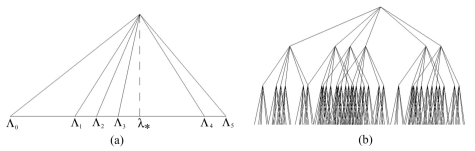
Figure 1. (a) The scheme of branching for $L=6$. (b) The tree for the third generation of a pre-fractal.

3. Multifractal integrals

Consider the fractals with $L$-branch multiplication (the case of dichotomous branching was considered in [1]). Having assigned the values

$$\lambda_{\ast}\in(0,1),\qquad 0\equiv\Lambda_{0}<\Lambda_{1}<\cdots\Lambda_{L-1}\equiv 1$$

and the contraction ratio $\kappa<1$, we choose the law of branching, shown in Figure 1, and define the multifractal integral of $f(x)$, with $x\in[0,1]$, as

(8) $$\int\limits_{\mathcal{L}}f(x)d\mu(x|\kappa,\Theta)=\lim\limits_{n\to\infty}\sigma_{n},\qquad\sigma_{n}=L^{-n}\sum\limits_{s}\Theta_{n}^{[s]}f(\lambda_{n}^{[s]}),$$

(existence and equality conditions for the limits in (8) are formulated below). The summation in (8) is made over all possible signature vectors $\mathbf{s}_{n}=(s_{n}^{(1)},\ldots,s_{n}^{(n)})$ with components $s_{n}^{(i)}\in\{\bar{\Lambda}_{0},\bar{\Lambda}_{1},\ldots,\bar{\Lambda}_{L-1}\}$ , where $\bar{\Lambda}_{k}=\Lambda_{k}-\lambda_{\ast}$. The arguments of the function $f$ are defined as follows

(9) $$\lambda_{n}^{[s]}=\lambda_{\ast}+(1-\kappa)(\mathbf{s}_{n},\mathbf{h}_{n}(\kappa)),$$

where ${\rm{\bf h}}_{n}(\kappa)=(1,\kappa,\kappa^{2},\ldots,\kappa^{n-1})$ and $({\rm{\bf a}},{\rm{\bf b}})=a_{1}b_{1}+\cdot\cdot\cdot+a_{n}b_{n}$, and the quantities $\Theta_{n}^{[s]}$ are functions of $\mathbf{s}_{n}$. Choosing normalization condition $\sigma_{n}=1$ for $f\equiv 1$ we find that

(10) $$\sum\limits_{k=0}^{L-1}\Theta_{n}^{[{s}^{k}]}=L\,\Theta_{n-1}^{[s]}$$

for $\mathbf{s}_{n}^{k}=\mathbf{s}_{n-1}\oplus(\bar{\Lambda}_{k})$ (where the $\oplus$ denotes a ”concatenation” of vectors). In this section we assume that the conditions

(11) $$\Theta_{n}^{[s]}=\prod\limits_{i=1}^{n}\psi(s_{n}^{(i)}),\qquad\sum\limits_{k=0}^{L-1}\psi(\bar{\Lambda}_{k})=L,$$

(12) $$\mbox{Im}\,\psi(\bar{\Lambda}_{k})=0,\qquad\mbox{Re}\,\psi(\bar{\Lambda}_{k})>0,$$

hold. In this case one can interpret $p_{k}=\psi(\bar{\Lambda}_{k})/L$ as probabilities; the corresponding multifractal measures induced by the multiplicative Besikovitch process were considered in [2]. Setting $X_{i}=(1-\kappa)(\lambda_{\ast}+\bar{\Lambda}_{i})$, we represent the solution of Eq.(5) (the Fourier transform of (7)) through the MFI

$$P_{\mbox{\scriptsize{st}}}(X)=\int\limits_{\mathcal{L}}P_{\mbox{\scriptsize{g}}}(X-x)d\mu(x|\kappa,\Theta).$$

The following existence conditions hold for MFI:

Theorem 1. If a function $f(x)$, $x\in[0,1]$, is continuous and conditions (11), (12) hold, the sequences of the quantities $\sigma_{n}$ in (8) converge to a limit equal to MFI.

Proof. For certain $n$, the summation in (8) goes over the points of the $n$-th generation pre-fractal, which is the set of $L^{n}$ points with coordinates $\lambda_{n}^{[s]}\in(0,1)$. By arranging the pre-fractals on parallel lines and connecting the points according to the rule $\mathbf{s}_{n}\Rightarrow\mathbf{s}_{n+1}^{k}=\mathbf{s}_{n}\oplus(\bar{\Lambda}_{k})$, $k=0,\ldots L-1$, we get a graph that represents the formation of the Cantor set for $n\to\infty$. Let the graph contains pre-fractals of first $n+k$ generations. One can see that every point of the $n$-th generation pre-fractal is a parent vertex for a cluster containing a tree of the subsequent generations. The corresponding rule of branching is given by

$$\lambda_{n+k}^{[s\oplus r]}=\lambda_{n}^{[s]}+\Delta_{n,k}^{[r]},\qquad\Delta_{n,k}^{[r]}=(1-\kappa)\kappa^{n}\left(\mathbf{r}_{k},\mathbf{h}(\kappa)\right);$$

$$-\kappa^{n}\,\lambda_{\ast}<\Delta_{n,k}^{[r]}<\kappa^{n}\,(1-\lambda_{\ast}).$$

As $k\to\infty$, every ”small” cluster converges to a Cantor fractal, which is similar to the full fractal.

Using definition (8) and conditions (11), we obtain

(13) $$|\sigma_{n+k}-\sigma_{n+k^{\prime}}|\leq|\sigma_{n+k}-\sigma_{n}|+|\sigma_{n+k^{\prime}}-\sigma_{n}|,$$

(14) $$\sigma_{n+k}-\sigma_{n}=\sum\limits_{s}L^{-n}\Theta_{n}^{[s]}\sum\limits_{r}L^{-k}\Theta_{k}^{[r]}\left(f(\lambda_{n}^{[s]}+\Delta_{n,k}^{[r]})-f(\lambda_{n}^{[s]})\right).$$

Taking into account that $|\Theta_{n}^{[s]}|\leq 1$, we get an estimate

(15) $$|\sigma_{n+k}-\sigma_{n}|\leq\sum\limits_{s}L^{-n}\Theta_{n}^{[s]}\sum\limits_{r}L^{-k}\Theta_{k}^{[r]}\left|f(\lambda_{n}^{[s]}+\Delta_{n,k}^{[r]})-f(\lambda_{n}^{[s]})\right|.$$

Let $f(x)$ be continuous on the closed interval $[0,1]$ (thus, uniformly continuous):

$$\forall x\in[0,1]\quad\forall\epsilon>0\quad\exists\delta_{\epsilon}\quad(\forall\alpha:\,|\alpha|<\delta_{\epsilon}):\quad|f(x+\alpha)-f(x)|<\epsilon/2.$$

Using the condition

$$\left[\lambda_{n}^{[s]}-\kappa^{n}\lambda_{\ast},\,\lambda_{n}^{[s]}+\kappa^{n}(1-\lambda_{\ast})\right]\subset\left[\lambda_{n}^{[s]}-\delta_{\epsilon},\,\lambda_{n}^{[s]}+\delta_{\epsilon}\right],$$

we can select $N_{\epsilon}$ for every $\delta_{\epsilon}$. Employing the relations (11) and (13)-(15), we obtain:

$$\forall\epsilon>0\quad\exists N_{\epsilon}\quad\forall n>N_{\epsilon}:\quad|\sigma_{n+k}-\sigma_{n+k^{\prime}}|<\epsilon,$$

showing that $\{\sigma_{n}\}$ is a Cauchy sequence and thus converges. $\blacksquare$

We find an alternative representation for the MFI using the singular distributions approach. Introducing singular functions

(16) $$\mathfrak{M}_{n}(x|\kappa,\Theta)=L^{-n}\sum\limits_{s}\Theta_{n}^{[s]}\,\delta(x-\lambda_{n}^{[s]}),\qquad\mathfrak{M}(x|\kappa,\Theta)=\lim\limits_{n\to\infty}\mathfrak{M}_{n}(x|\kappa,\Theta),$$

we have:

$$\int\limits_{\mathcal{L}}f(x)d\mu(x|\kappa,\Theta)=\int\limits_{0}^{1}f(x)\,\mathfrak{M}(x|\kappa,\Theta)dx\equiv\lim\limits_{n\to\infty}\int\limits_{0}^{1}f(x)\,\mathfrak{M}_{n}(x|\kappa,\Theta)dx.$$

The Fourier transform of the limit in (16) is a solution of a dilatation equation

$$\hat{\mathfrak{M}}(\omega|\kappa,\Theta)=\hat{\mathfrak{N}}(\omega|\kappa,\Theta)\,\hat{\mathfrak{M}}(\kappa\omega|\kappa,\Theta),$$

$$\hat{\mathfrak{N}}(\omega|\kappa,\Theta)=L^{-1}\,\sum\limits_{k=0}^{L-1}\Psi(\bar{\Lambda}_{k})\exp\left\{-i\omega(1-\kappa)(\lambda_{\ast}+\bar{\Lambda}_{k})\right\}$$

and is equal to

$$\hat{\mathfrak{M}}(\omega|\kappa,\Theta)=e^{-i\omega\lambda_{\ast}}\prod\limits_{\gamma=0}^{\infty}\left[L^{-1}\,\sum\limits_{k=0}^{L-1}\Psi(\bar{\Lambda}_{k})\exp\left\{-i\omega(1-\kappa)\kappa^{\gamma}\,\bar{\Lambda}_{k}\right\}\right].$$

Accordingly, the dilatation equation for the limit function (16) reads:

$$\mathfrak{M}(x|\kappa,\Theta)={\kappa}^{-1}\int\limits_{-\infty}^{\infty}\mathfrak{N}(x-y|\kappa,\Theta)\,\mathfrak{M}\left(\kappa^{-1}y|\kappa,\Theta\right)dy,$$

$$\mathfrak{N}(x|\kappa,\Theta)=L^{-1}\,\sum\limits_{k=0}^{L-1}\Psi(\bar{\Lambda}_{k})\,\delta\left(x-(1-\kappa)(\lambda_{\ast}+\bar{\Lambda}_{k})\right).$$

It is possible to define the MFI as a limit of a sequence of definite integrals. Such definition is more illustrative but in fact is equivalent to (8)-(12). This approach was developed in [1] for $L=2$. Here we present this formalism briefly.

Define the MFI as

(17) $$\int\limits_{\mathcal{L}}f(x)d\mu(x|\kappa,\Theta)=\lim\limits_{n\to\infty}\sigma_{n}^{\#},\qquad\sigma_{n}^{\#}=2^{-n}\sum\limits_{s}\Theta_{n}^{[s]}\prec\!\!f\left(\lambda_{n}^{[s]}\right)\!\!\succ\!\!{\vphantom{()}}_{\kappa^{n}}\,,$$

where

$$\prec\!\!{f(x)}\!\!\succ\!\!{\vphantom{()}}_{\delta}={\delta}^{-1}\int_{x-\delta/2}^{x+\delta/2}f(t)dt$$

and $\lambda_{n}^{[s]}$ is defined by (9) with $L=2$, $\lambda_{\ast}=\tfrac{1}{2}$, $\Lambda_{0}=0$, $\Lambda_{1}=1$. For $\kappa<\tfrac{1}{2}$, $\sigma_{n}^{\#}$ is computed by integration over a system of nonintersecting segments $\mathcal{L}_{n}=\bigcup_{s}l_{n}^{[s]}\subset[0,1]$, where $l_{n}^{[s]}=[\,\lambda_{n}^{[s]}-\tfrac{1}{2}\kappa^{n},\lambda_{n}^{[s]}+\tfrac{1}{2}\kappa^{n}\,]$. The set $\mathcal{L}_{n}$ is obtained from the unit segment by the standard Cantor procedure repeated $n$ times: one first removes from the unit segment a middle part of length $1-2\kappa$, then the same fraction is removed from the middle of each of the remaining segments, and so forth. The measure is constructed by assigning to each segment $l_{n}^{[s]}$ a weight factor $\Theta_{n}^{[s]}$ appearing in the summation in (17).

The helpful intuitive picture of the pre-fractal domain $\mathcal{L}_{n}$ and the cluster set $\mathcal{L}=\lim_{n\to\infty}\mathcal{L}_{n}$ embedded in $[0,1]$ is no longer valid for $\tfrac{1}{2}<\kappa<1$, since the segments $l_{n}^{[s]}$ intersect in that case. This difficulty may be resolved by replacing the segments with rectangles and ”spreading” them along the second coordinate. Define two-dimensional MFI of $f(x,y)$, $x\in[0,1]$, $y\in[0,1]$ as follows

(18) $$\iint\limits_{\mathcal{D}}f(x,y)d\mu(x,y|\kappa_{x},\kappa_{y},\Theta)=\lim\limits_{n\to\infty}2^{-n}\sum\limits_{s}\Theta_{n}^{[s]}\left\langle f\left(\lambda_{xn}^{[s]},\lambda_{yn}^{[s]}\right)\right\rangle_{\kappa_{x}^{n},\kappa_{y}^{n}}.$$

We assume that $\lambda_{\alpha n}^{[s]}$ is determined by the expression that follows from (9) by replacing $\kappa$ with $\kappa_{\alpha}$, $\alpha=x,y$, and that the average is taken over the region $d_{n}^{[s]}=l_{xn}^{[s]}\otimes l_{yn}^{[s]}$, $l_{\alpha n}^{[s]}=[\,\lambda_{\alpha n}^{[s]}-\tfrac{1}{2}\kappa_{\alpha}^{n},\lambda_{\alpha n}^{[s]}+\tfrac{1}{2}\kappa_{\alpha}^{n}\,]$. The rectangular cells $d_{n}^{[s]}$ do not overlap if at least one of the contraction coefficients $\kappa_{\alpha}$, $\alpha=x,y$, is not larger than $\tfrac{1}{2}$. This condition is satisfied, in particular, for $\kappa_{x}=\kappa$, $0<\kappa<1$, and $\kappa_{y}=\tfrac{1}{2}$, and then

$$\iint\limits_{\mathcal{D}}f(x)d\mu(x,y|\kappa,\tfrac{1}{2},\Theta)=\int\limits_{\mathcal{L}}f(x)d\mu(x|\kappa,\Theta).$$

If $\kappa_{\alpha}\leq\tfrac{1}{2}$ for $\alpha=x$ (for $\alpha=y$), the projection of $\mathcal{D}=\lim_{n\to\infty}\bigcup_{s}d_{n}^{[s]}$ onto the $x$ (the $y$) axis is a standard Cantor set that has the similarity dimension $D_{\alpha}=-\left(\log_{2}\kappa_{\alpha}\right)^{-1}$. As it was shown in [2], the Hausdorff-Besicovitch dimension $D$ of the whole set $\mathcal{D}$ is equal to $D=2/(1-\log_{2}\kappa)$. Note that for $\kappa=\tfrac{1}{2}$ we have $D=1$; in this case $\mathcal{D}$ is a diagonal of the unit square, and (18) reduces to a definite integral on the diagonal.

4. The nonlinear Ikeda mapping

Consider a circuit with a nonlinear element and a delayed feedback [1, 3, 4, 5, 6, 7, 8]. Assuming $\xi^{\mbox{\scriptsize{fl}}}(t)$ being a random process with zero mean value $\langle\!\langle\xi^{\mbox{\scriptsize{fl}}}(t)\rangle\!\rangle=0$, we can write a stochastic difference equation

(19) $$X(t)=F(X(t-T_{\mbox{\scriptsize{del}}}))+\xi^{\mbox{\scriptsize{fl}}}(t-T_{\mbox{\scriptsize{del}}}),$$

where $T_{\mbox{\scriptsize{del}}}$ is the delay time. For $X(t)$ being a two-dimensional (complex) signal, the equation (19) can be rewritten in the form of mapping (1), where $X_{N}=X(t_{0}+NT_{\mbox{\scriptsize{del}}})$, $\xi_{N}^{\mbox{\scriptsize{fl}}}=\xi(t_{0}+(N+1)T_{\mbox{\scriptsize{del}}})$, $0\leq t_{0}<T_{\mbox{ \scriptsize{del}}}$ (in this case $\langle X,U\rangle=\mbox{Re }(XU^{*})$). Suppose that the external noise is the Ornstein-Uhlenbeck random process with small correlation time $\tau_{\mbox{\scriptsize{cor}}}\ll T_{\mbox{\scriptsize{del}}}$ (the ”rapid” Gaussian noise). Assuming the transformation of a slowly varying complex valued amplitude $X(t)$ as a phase shift $\phi\to\phi+\lambda{|X|}^{2}+\theta_{0}$ and the dissipative contraction $|X|\to\kappa|X|$, $\kappa<1$, we find the nonlinear term in (1), (19) in the form

(20) $$F(X)=1+\kappa X\exp(i\lambda\left|X\right|^{2}+i\theta_{0})$$

(the Ikeda mapping [3, 4]). As shown in [5, 6, 7], the random phase approximation can be used in the intence phase mixing limit $\lambda\gg 1$, which allows to replace the delta-function in (2) by

$$\delta^{(2)}(Y-F(Z))\longrightarrow\langle\!\langle\,\delta^{(2)}(Y-1-\kappa Ze^{i\phi})\,\rangle\!\rangle_{\phi},$$

where $\langle\!\langle\cdots\rangle\!\rangle_{\phi}$ denotes an average over $\phi$. Then

$$P_{\mbox{\scriptsize{st}}}(X)=\int dY\,P_{\mbox{\scriptsize{g}}}\left(X-Y,R/(1-\kappa^{2})\right)P_{\mbox{\scriptsize{ch}}}(Y).$$

The radially symmetric distribution $P_{\mbox{\scriptsize{ch}}}$ describing noise caused by dynamic chaotization [5, 6, 7] can be written in the form

(21) $$P_{\mbox{\scriptsize{ch}}}(X)=(2\pi\kappa^{2})^{-1}\int_{0}^{\infty}\beta d\beta\,\,\Xi(\beta)\,J_{0}\left(\beta\kappa^{-1}\left|X-1\right|\right)$$

(22) $$\Xi(\beta)=J_{0}(\beta)\Xi(\kappa\beta),\qquad\qquad\Xi(\beta)=\prod\limits_{k=0}^{\infty}J_{0}(\beta\kappa^{k}).$$

The integrand in (21) contains a factor $\Xi(\beta)$ which is a solution of the dilatation equation (22). In order to simplify (21), (22), we approximate the Bessel function by a function with separated ”oscillatory” and monotonic parts $J_{0}(x)\approx\chi(x)\left[\sqrt{2}\cos\left(x-\tfrac{1}{4}\pi\right)\right]$. In this approximation

$$f_{\mbox{\scriptsize{ch}}}(Q)\approx\frac{1}{\sqrt{2}}\left\{e^{-i\pi/4}\int\limits_{\mathcal{L}}\hat{\Phi}\!\left(\!\sqrt{Q}+\frac{2x-1}{1-\kappa},\,Q\!\right)\,d\mu(x|\kappa,\Theta)+\mbox{c.c.}\right\},$$

$$\Phi(\beta,Q)=\frac{1}{2}\beta\,\chi\!\left(\beta\sqrt{Q}\right)\prod\limits_{k=0}^{\infty}\chi\!\left(\beta\kappa^{k}\right),\qquad\Theta_{n}^{[s]}=2^{n/2}\exp\left[-\tfrac{1}{4}i\pi({\rm{\bf s}}_{n},{\rm{\bf h}}_{n}(1))\right],$$

where $\hat{\Phi}$ is the Fourier transform w.r.t. first argument of the monotonic function $\Phi$. Notice that quantities $\Theta_{n}^{[s]}$ fail to satisfy the conditions (12). Thus the Theorem 1 does not hold and we have to look for an alternative condition of convergence.

5. Extended class of multifractal integrals

Let us consider the definition (8) of the MFI without the condition (12). Now we assume that $\Psi(\bar{\Lambda}_{k})$ are complex-valued.

Theorem 2. Let the function $f(x)$, $x\in[0,1]$, be differentiable arbitrary many times, also let $\exists M\,\,\forall x\,\,\forall l\in\mbox{{N}}:\,\,|f^{(l)}(x)|<M$, and let the conditions (11) hold. Then the sequences $\sigma_{n}$ in (8) converge to a limit equal to MFI.

Proof. Taking into account the formula (9) and introducing the power expansion

$$f(\lambda_{n}^{[s]})=\sum\limits_{l=0}^{\infty}\frac{1}{l!}f^{(l)}(\lambda_{\ast})(1-\kappa)^{l}\left(\mathbf{s}_{n},\,\mathbf{h}_{n}(\kappa)\right)^{l},$$

we obtain

(23) $$|\sigma_{n}|\leq\sum\limits_{l=0}^{\infty}\frac{1}{l!}|f^{(l)}(\lambda_{\ast})|\,(1-\kappa)^{l}\,\Bigl{|}L^{-n}\sum\limits_{s}\Theta_{n}^{[s]}\left(\mathbf{s}_{n},\,\mathbf{h}_{n}(\kappa)\right)^{l}\Bigr{|}.$$

The use of the generating function for the powers of the scalar product $\exp\{\xi(\mathbf{s}_{n},\,\mathbf{h}_{n}(\kappa))\}$ and the Leibnitz formula allows us to perform the transformations:

$$L^{-n}\sum\limits_{s}\Theta_{n}^{[s]}\left(\mathbf{s}_{n},\,\mathbf{h}_{n}(\kappa)\right)^{l}=\Bigl{.}\frac{d^{l}}{d\xi^{l}}\Bigl{(}L^{-n}\sum\limits_{s}\Theta_{n}^{[s]}\,\,e^{\,\xi\,(\mathbf{s}_{n},\,\mathbf{h}_{n}(\kappa))}\Bigr{)}\Bigr{|}_{\xi=0}$$

$$=\Bigl{.}\frac{d^{l}}{d\xi^{l}}\Bigl{(}\prod\limits_{j=1}^{n}\Bigl{[}L^{-1}\sum\limits_{k=0}^{L-1}\Psi(\bar{\Lambda}_{k})\,e^{\,\xi\,\kappa^{j-1}\bar{\Lambda}_{k}}\Bigr{]}\Bigr{)}\Bigr{|}_{\xi=0}$$

(24) $$=\sum\limits_{m}\,\left(m_{1},\ldots m_{n}\right)!\,\prod\limits_{j=1}^{n}\Bigl{(}\kappa^{m_{j}(j-1)}\Bigl{[}L^{-1}\sum\limits_{k=0}^{L-1}\Psi(\bar{\Lambda}_{k})\bar{\Lambda}_{k}^{m_{j}}\Bigr{]}\Bigr{)}.$$

The left summation in (24) goes over all non-negative integers $m_{i}$ that satisfy the condition $\sum_{i=0}^{n}m_{i}=l$, and $(m_{1}\ldots m_{n})!=(m_{1}+\cdots+m_{n})!/(m_{1}!\cdots m_{n}!)$ are the multinomial coefficient. The inequality $|\bar{\Lambda}_{k}|=|\Lambda_{k}-\lambda_{\ast}|<1$ implies $|\bar{\Lambda}_{k}^{m}|<1$, $m\in\mbox{{N}}$. This allows us to obtain the upper estimates

$$\Bigl{|}L^{-1}\sum\limits_{k=0}^{L-1}\Psi(\bar{\Lambda}_{k})\bar{\Lambda}_{k}^{m}\Bigr{|}\leq\max\limits_{|\beta_{k}|<1}\Bigl{|}L^{-1}\sum\limits_{k=0}^{L-1}\Psi(\bar{\Lambda}_{k})\beta_{k}\Bigr{|}=G_{1}\leq G,$$

where $G=\max\{G_{1},\,1\}$. Notice that the number of multipliers $L^{-1}\sum_{k=0}^{L-1}\Psi(\bar{\Lambda}_{k})\bar{\Lambda}_{k}^{m}$ with $m\neq 0$ in (24) does not exceed the least of the numbers $n$ and $l$. This allows us to write a sequence of upper estimates:

(25) $$\Bigl{|}L^{-n}\sum\limits_{s}\Theta_{n}^{[s]}\left(\mathbf{s}_{n},\,\mathbf{h}_{n}(\kappa)\right)^{l}\Bigr{|}\leq\sum\limits_{m}\,\left(m_{1},\ldots m_{n}\right)!\,\prod\limits_{j=1}^{n}\Bigl{(}\kappa^{m_{j}(j-1)}\Bigl{|}L^{-1}\sum\limits_{k=0}^{L-1}\Psi(\bar{\Lambda}_{k})\bar{\Lambda}_{k}^{m_{j}}\Bigr{|}\Bigr{)}$$

(26) $$\leq G^{l}\,\sum\limits_{m}\,\left(m_{1},\ldots m_{n}\right)!\,\prod\limits_{j=1}^{n}\kappa^{m_{j}(j-1)}\leq G^{l}(1-\kappa)^{-l}.$$

As result, we see from (23), (25) and (26) that

(27) $$|\sigma_{n}|\leq\sum\limits_{l=0}^{\infty}\frac{1}{l!}|f^{(l)}(\lambda_{\ast})|\,G^{l}\leq M\,\sum\limits_{l=0}^{\infty}\frac{1}{l!}G^{l}=M\,e^{G}.$$

Taking into account the relations (13)-(15), (25)-(27), we find:

$$|\sigma_{n+k}-\sigma_{n}|=\Bigl{|}\sum\limits_{s}L^{-n}\Theta_{n}^{[s]}\sum\limits_{r}L^{-k}\Theta_{k}^{[r]}\left(f(\lambda_{n}^{[s]}+\Delta_{n,k}^{[r]})-f(\lambda_{n}^{[s]})\right)\Bigr{|}$$

$$\leq\Bigl{|}\sum\limits_{l=1}^{\infty}\frac{1}{l!}\Bigl{(}\sum\limits_{s}L^{-n}\Theta_{n}^{[s]}f^{(l)}(\lambda_{n}^{(s)})\Bigr{)}\,\Bigl{(}\sum\limits_{k}L^{-k}\Theta_{k}^{[r]}(\Delta_{n,k}^{(s)})^{l}\Bigr{)}\Bigr{|}$$

$$\leq\sum\limits_{l=1}^{\infty}\frac{1}{l!}\Bigl{|}\sum\limits_{s}L^{-n}\Theta_{n}^{[s]}f^{(l)}(\lambda_{n}^{(s)})\Bigr{|}\,\kappa^{nl}(1-\kappa)^{l}\Bigl{|}\sum\limits_{r}L^{-k}\Theta_{k}^{[r]}\left(\mathbf{r}_{k},\,\mathbf{h}_{k}(\kappa)\right)^{l}\Bigr{|}$$

$$\leq M\,e^{G}\,\sum\limits_{l=1}^{\infty}\frac{1}{l!}G^{l}\kappa^{nl}\leq Me^{G}\,(e^{G\kappa^{n}}-1).$$

We see that

$$\forall\epsilon>0\quad\exists N_{\epsilon}\quad\forall n>N_{\epsilon}:\quad|\sigma_{n+k}-\sigma_{n+k^{\prime}}|<2Me^{G}\,(e^{G\kappa^{n}}-1)<\epsilon,$$

which implies convergence of the Cauchy sequence $\{\sigma_{n}\}$. $\blacksquare$

6. Random processes transformations in a circuit with dissipation and delayed feedback.

Consider a circuit described by the equations (19), (20) in assumption that $\tau_{\mbox{\scriptsize{ cor}}}\sim T_{\mbox{\scriptsize{del}}}$ [5, 6, 7, 8]. This situation is more difficult for analysis as one should take into account correlations between the variables $\xi_{N}^{\mbox{\scriptsize{fl}}}=\xi(t_{0}+(N+1)T_{\mbox{\scriptsize{del}}})$ with different $N$. Now we are forced to seek the stationary solution of the generalized Kolmogorov-Chapman equation for the multi-time distribution functions:

(28) $$P_{\mbox{\scriptsize{st}}}((X_{s}),\xi_{n+1})=\int d\boldsymbol{Y}d\boldsymbol{\xi}\,P_{\mbox{\scriptsize{st}}}((Y_{s}),\xi_{0})$$

$$\qquad\qquad\times\prod\limits_{p=0}^{n}\delta^{(2)}(X_{p}-\xi_{p}-F(Y_{p}))\,w(\xi_{p+1},\xi_{p},[\tau_{p+1}-\tau_{p}]).$$

In (28) we use a short-hand notation

$$P_{N}((X_{s}),\xi)=P((X_{0}[NT_{\mbox{\scriptsize{del}}}],\,X_{1}[NT_{\mbox{\scriptsize{del}}}+\tau_{1}],\cdots,X_{n}[NT_{\mbox{\scriptsize{del}}}+\tau_{n}]),\,\xi[NT_{\mbox{\scriptsize{del}}}]),$$

where $X_{i},\,i=0,1,...,n$, are the signal amplitudes at $NT_{\mbox{ \scriptsize{del}}}+\tau_{i}$, respectively, and $\xi$ denotes the amplitude of $\xi^{\mbox{\scriptsize{fl}}}$ at $NT_{\mbox{\scriptsize{ del}}}$. We also require $0=\tau_{0}<\tau_{1}<\cdots<\tau_{n}<\tau_{n+1}=T_{\mbox{\scriptsize{del}}}$ and use a notation $d\boldsymbol{A}\equiv dA_{0}\,dA_{1}\,dA_{2}\ldots$. The noise term $\xi^{\mbox{\scriptsize{fl}}}$ is assumed to be the Markovian random process with arbitrary $\tau_{\mbox{\scriptsize{ cor}}}$ and the transition density function $w(\xi,\xi^{\prime},[\tau])$ (the Ornstein-Uhlenbeck and Kubo-Andersen random process were treated in [6, 7, 8]). The equation for the distribution function Fourier transform reads

(29) $$\psi_{\mbox{\scriptsize{st}}}((U_{s}),\Omega_{n+1})=\int d\boldsymbol{V}d\boldsymbol{\Omega}\,\psi_{\mbox{\scriptsize{st}}}((V_{s}),\Omega_{0})$$

$$\qquad\qquad\times\prod\limits_{p=0}^{n}\sigma(U_{p},V_{p})\,H(\Omega_{p+1},\Omega_{p}-U_{p},[\tau_{p+1}-\tau_{p}]),$$

where $H(\Omega,\Omega^{\prime},[\tau])$ is the Fourier transform of $w(\xi,\xi^{\prime},[\tau])$ and the function $\sigma(U,V)$ is defined by (4). This function may be written in the form

$$\sigma=\bar{\sigma}+\Delta\sigma,\quad\bar{\sigma}\left(U,V\right)=\left(2\pi\left|V\right|\right)^{-1}e^{-i\,\mbox{\scriptsize{Re}}U}\delta\left(\left|V\right|-\kappa\left|U\right|\right),$$

where the first term $\bar{\sigma}$ corresponds to the random phase approximation and describes the case of chaotic motion with intense phase mixing [7, 8]. This means that in the limit $\lambda\to\infty$ in (20) one can replace $\sigma$ by $\bar{\sigma}$ (respective approximate solution of (28), (29) are labeled by superscript (0)). The exact and approximate forms of (28) can be presented in the operator form:

(30) $$\psi_{\mbox{\scriptsize{st}}}=\left({\bf\hat{K}}+\varepsilon{\bf\hat{S}}\right)\psi_{\mbox{\scriptsize{st}}}\quad\xrightarrow{\sigma\to\bar{\sigma},\quad\mbox{random phase approx.}}\quad\psi_{\mbox{\scriptsize{st}}}^{\left(0\right)}={\bf\hat{K}}\psi_{\mbox{\scriptsize{st}}}^{\left(0\right)}.$$

In case of the Ornstein-Uhlenbeck random process [8] the explicit formula for ${\bf\hat{K}}$ takes the form:

(31) $${\bf\hat{K}}f((U_{s}),U_{n+1})=\Bigl{[}\>\prod\limits_{p=0}^{n}e^{-i\,\mbox{\scriptsize{Re}}U_{p}}\Bigr{]}\Phi((U_{s}),U_{n+1})\left\langle\!\!\!\left\langle f\Bigl{(}(\kappa U_{s}e^{i\phi_{s}}),\sum\limits_{q=0}^{n+1}\theta_{\tau_{q}}U_{q}\Bigr{)}\right\rangle\!\!\!\right\rangle_{\phi_{s}},$$

$$\Phi((U_{s}),U_{n+1})=\exp\Bigl{\{}-\frac{R}{4}\,\sum\limits_{p=1}^{n+1}{\Bigl{|}\sum\limits_{q=p}^{n+1}\frac{\theta_{\tau_{q}}}{\theta_{\tau_{p}}}U_{q}\Bigr{|}^{2}}\Bigl{(}1-\frac{\theta_{\tau_{p}}^{2}}{\theta_{\tau_{p-1}}^{2}}\Bigr{)}\Bigr{\}}.$$

It is evident that the operator ${\bf\hat{K}}$ produces a scaling transformation (dilatation), because the right-hand side of (31) contains the functions with scaled arguments $\kappa U_{s}$. Thus the right equation in (30) is a generalized dilatation equation. The equation (28) may be viewed as an equation with the ”small” operator $\varepsilon{\bf\hat{S}}$. This enables to obtain the solution in the form of a series expansion. Taking into account the normalization conditions $\psi_{\mbox{ \scriptsize{st}}}\left(\left(0\right),0\right)=\psi_{\mbox{ \scriptsize{st}}}^{\left(0\right)}\left(\left(0\right),0\right)=1$, one finds

$$\psi_{\mbox{\scriptsize{st}}}^{\left(0\right)}\left(\left(U_{s}\right),\Omega\right)=\lim_{m\rightarrow\infty}{\bf\hat{K}}^{m}\,{\bf 1},\qquad\qquad\qquad\psi_{\mbox{\scriptsize{st}}}=\psi_{\mbox{\scriptsize{st}}}^{\left(0\right)}+\sum\limits_{j=1}^{\infty}\varepsilon^{j}\Bigl{\{}\Bigl{(}\sum\limits_{p=0}^{\infty}{\bf\hat{K}}^{p}\Bigr{)}{\bf\hat{S}}\Bigr{\}}^{j}\psi_{\mbox{\scriptsize{st}}}^{\left(0\right)}.$$

This approach was developed in [8] where the criterion of convergence was examined.

Acknowledgements

VZ acknowledges the financial support from the European Mathematical Society.

References

[1] Zverev V.V., On the conditions for the existence of
fractal domain integrals, Theor. Math. Phys.107, (1996), 419-426.
[2] Feder J., Fractals, Plenum press, 1988.
[3] Ikeda K., Daido H., Akimoto O., Optical Turbulence:
chaotic behavior of transmitted light from a ring cavity, Phys. Rev. Lett.45, (1980), 709-712.
[4] Singh S., Agarwal G.S., Chaos in coherent
two-photon processes in a ring cavity, Opt. Comm.47, (1983), 73-76.
[5] Zverev V.V., Rubinstein B.Y., Random self-modulation of radiation
in a ring cavity: Case of strong mixing Opt. Spect.65, (1988), 971-978.
[6] Zverev V.V., Rubinstein B.Y., Autostochasticity and
conversion of lasing fluctuations in a ring cavity with a nonlinear element,
Opt. Spect.70, (1991), 1305-1311.
[7] Zverev V.V., Rubinstein B.Y., Chaotic oscillations and noise
transformations in a simple dissipative system with delayed feedback,
J. Stat. Phys.63, (1991), 221-239.
[8] Zverev V. V., Noise transformation in nonlinear system with intensity
dependent phase rotation, Stochastics and Dynamics.3, (2003), 421-433.