Example of a possible interpretation of Tsallis entropy

Abstract: We demonstrate and discuss the process of gaining information and show an example in which some specific way of gaining information about an object results in the Tsallis form of entropy rather than in the Shannon one.

PACS: 05.20.-y; 05.70.-a; 05.70.Ce

Keywords: Nonextensive statistics, Correlations, Fluctuations

Some time ago the notion of information in the form dictated by Shannon entropy [1] was used by us to study multiparticle production processes [2]. Later we found that its Tsallis version [3] is more suitable [5], because the nonextensivity parameter $q$ characterizing Tsallis entropy bears information about the intrinsic fluctuations in the physical system [6]. The finding that $q$ can be interpreted as a measure of such fluctuations resulted in a new subject called superstatistics dealing with all kinds of fluctuation, see [7]. In all these studies we used either the Shannon or Tsallis form of information entropy without, however, any deeper understanding or argumentation about what in fact makes them so different, i.e., without deeper thoughts about the details of the process of gaining information leading to one or another form of information entropy.

In this note we shall concentrate on this problem, using as our basic tool a widely known example presented in [8]) which demonstrates how to deduce in a simple manner the form of Shannon informational entropy by considering the process of finding the location of some object in a prescribed phase space (like, for example, a point on a sheet of paper). We shall develop an equivalent procedure resulting in Tsallis entropy instead. In particular we shall demonstrate, using these examples, how the way in which one collects information about an object decides the form of the corresponding information entropy. As already mentioned above we shall concentrate only on the comparison between Shannon [1] ($S=S_{q=1}$) and Tsallis [3] ($S_{q}=S_{q\neq 1}$) forms of entropy:

$$S=-\sum_{i}p_{i}\ln p_{i}\qquad\Leftrightarrow\qquad S_{q}=-\sum_{i}p_{i}\ln_{q}p_{i}=-\sum_{i}p_{i}\frac{\left(1-p^{q-1}_{i}\right)}{1-q}.$$ (1)

Acting in the same spirit as in [8], consider a system of size $V_{0}$ and divide it into cells of size $V$ each; we then have $M=V_{0}/V$ such cells (divisions). Suppose now that in one of these cells an object is hidden (we shall call it a particle in what follows) and that the probability to find it in a cell is the same for all cells and equal $\frac{1}{M}$. The corresponding Shannon entropy, describing the situation of finding this particle in one of the cells, is:

$$S=-\sum_{i=1}^{M}\frac{1}{M}\ln\left(\frac{1}{M}\right).$$ (2)

Suppose that the cells were formed by consecutively dividing previous cells into two equal parts and that we have performed $f$ such divisions. Then $M=2^{f}$ and Shannon entropy (2) corresponds conventionally to $S=\log_{2}M=f$ bits of information. The tacit assumption is that to locate a particle in the system is equivalent to finding the respective cell containing this particle. In such an approach, entropy equals just the number of YES/NO questions needed to locate the selected particle. In a sense, our particle is structureless, i.e., it has no additional features which would have to be investigated before its proper recognition; the localization of the particle is therefore equivalent with its recognition.

Suppose, however, that the particles we are searching for have some additional features one has to account for and that in a cell there can be more (or less) than one particle. It is obvious that in such a case the localization of the cell as performed above is not equivalent to the recognition of the right particle itself. One can now be faced with two situations:

• One finds the cell with a particle in it but one is still not sure that this is the right (”true”) particle; some additional search involving additional features mentioned above is required - one needs more information than in the usual case.

• One recognizes the right particle already before the search of the proper cell is finished, it means that some information offered is redundant - one needs less information than in the usual case.

The problem now is: how to quantify this problem? There is a priori an enormous number of factors which result in those additional features which should apparently be accounted for. On the other hand, from our point of view, all of them are, in a sense, identical because they simply transform the originally structureless particle to a particle endowed with some structure which can vary from one particle to the other. Let us therefore concentrate on a simplest possibility and assume that it is enough to replace the single particle considered originally in [8] by a number of identical particles endowed with some artificial size $\nu$, which can occupy each cell. Identical means therefore that all particles have the same size which they keep all the time. Notice that:

• in the whole volume $V_{0}$ considered one can only put $N=V_{0}/\nu$ particles;

• in a given cell one can only put $k=V/\nu$ particles; it is very important to realize that one can have $k>1$ as well as $k<1$ (in addition to the original case corresponding to $k=1$).

As before we again attempt to locate the selected particle in our system in a most effective way (i.e., by using only the minimal possible amount of information). The probability to choose the cell with this particle is $p=1/M=V/V_{0}$. However, now the size of the particle matters and the cell can be occupied by a number of particles among which we must choose the one we are looking for. As illustrated in Fig. 1 one can encounter three typical situations:

• Even when one finds the right cell one still has to search for a while before deciding that the chosen particle is the right one. In our example this is visualized by the fact that the particle is smaller then the cell and there can be more than one particle per cell (notice that more does not mean here that the actual number is an integer, it can be any positive number), cf. left panel of Fig. 1.

• It can happen that one is sure that the chosen particle is the right one even before the right cell has been identified. In our example this corresponds to a situation when the particle is bigger than the cell. This means that the particle occupies more than one cell (again, more means that this is any real number greater than unity but smaller than the maximally allowed number of cells equal $V_{0}/V$), cf. right panel of Fig. 1.

• The information needed to locate the particle is the same as to find the right cell. In our example it simply means that volumes of cell and particle are equal and there can be only one particle per cell., cf. the middle panel of Fig. 1.

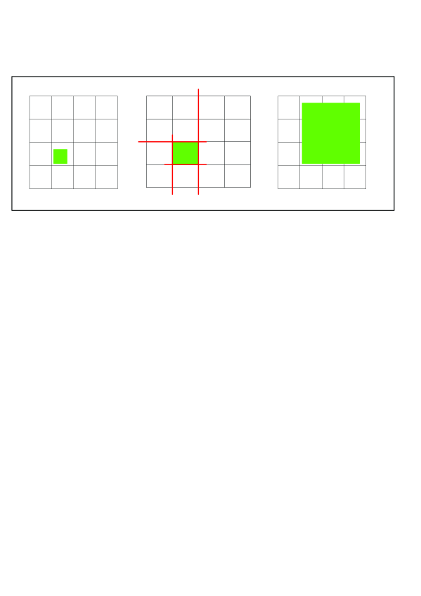
Figure 1: Schematic illustration of three possible situation encountered when gathering information. Left panel: whatever number of divisions the object we are looking for is smaller then the actual cell and can require some additional (in comparison to the usual) search. Middle panel: there is no additional information needed to locate the object. Right panel: object shows itself (and therefore can also be identified) already before the usual amount of search (i.e., divisions) is performed. Only the middle panel situation leads to the Shannon form of entropy, the remaining two result in the Tsallis entropy instead.

To continue along this line let us notice that one (chosen) particle can register in a cell with probability $p$ or not register in this cell with probability $1-p$. In the case when this particle is not identified with the cell (as is the case in the case of counting the Shannon entropy), in this cell there can be maximally $k-1$ other (false) particles. Assuming independence of events, the probability of the occurrence $r$ such particles in the cell is $p^{r}$. Therefore, on the average, the probability to register a false particle (and not the chosen one) per one false particle is

$$\langle p_{k-1}\rangle=\frac{1-p}{k-1}\sum^{k-1}_{r=1}p^{r}=-\frac{p}{k-1}\left(p^{k-1}-1\right).$$ (3)

Notice that by doing so we are also tacitly assuming that any false choice also removes (or equivalently marks somehow) the falsely chosen particle as misidentification.

Before proceeding further, a few words of conditions under which formula (3) may be valid are in order. Our picture could physically correspond to the situation in which we perform measurements with noise ($q>1$) or when errors connected with the measurement exceed the size of the cell ($q<1$). In this case our object is identified in a number of cells (in other words, in this case our cells are not ”mutually exclusive” as they were in the usual situation leading to Shannon entropy). One can also encounter a situation when the cells are not refined enough in phase space, equivalent to the case in which cells are exactly known but the location of our object (particle) is not fixed. All such situations eventually lead to Eq. (3).

To continue, the question we have to answer now is: what is the corresponding entropy in this case, or - what is the analogy to YES/NO questions in the previous case, where the number of questions was the entropy? We argue that the analogy to YES/NO questions in this case is the sum over all cells of the probability to not register the particle (i.e., probability to register only false particles). Notice that Eq. (3) gives us the gain of information we get from a single cell. For a system of $2$ cells, $i=1,2$, with $p_{1}=0$ and $p_{2}=1$ one has $H=0$, whereas for $0<p_{i}<1$ one gets $H>0$. Therefore one can say that the entropy for a system of $M$ cell is given by

$$H=\sum^{M}_{i=1}\langle p_{k-1}\rangle=-\sum^{M}_{i=1}p\frac{p^{k-1}-1}{k-1},$$ (4)

which in our case can be rewritten in the following form,

$$H=-\sum^{M}_{i=1}\frac{V}{V_{0}}\frac{\left(\frac{V}{V_{0}}\right)^{\frac{V}{\nu}-1}-1}{\frac{V}{\nu}-1}.$$ (5)

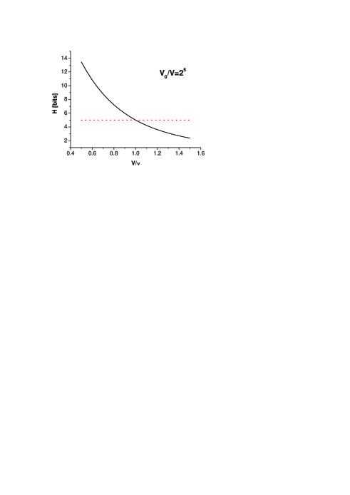
Figure 2: Illustration of the dependence of $H$ on $k=V/\nu$ for the number of cells equal to $V_{0}/V=2^{5}$ (full line). The Shannon entropy (dotted line) for the same number of cells is equal $S=5$ (because we have now $5$ bits). Notice that $H>S$ for $k<1$ and $H<S$ for $k>1$.

Notice that entropy defined by Eq. (4) or (5) is formally identical in its form with the Tsallis entropy [3] with $q=k=V/\nu$. Its behavior is illustrated in Fig. 2. It has the following characteristic properties:

• $H\rightarrow 0$ if $V\rightarrow V_{0}$, i.e., when one has just one cell (in this limit there is no information left in the system, see Fig. 2, $k>1$ case);

• When $\nu\rightarrow V_{0}$, i.e., when the particle we are looking for covers all cells (becoming therefore identical with the system itself), the entropy $H$ grows monotonically and reaches the limiting value

  $$H=\frac{M}{M-1}\left(M^{1-1/M}-1\right)<M.$$ (6)

  It is interesting to note that when $M$ becomes very large then $H\longrightarrow M$ in this limit. This should be contrasted with the much milder behavior of Shannon entropy which in this limit becomes $S\propto\ln M$ (cf. Fig. 2, $k<1$ case). The difference arises because in this case in order to fully identify a particle in the system one must go through all cells with positive outcome, not only through a sunset of them as is done in the procedure leading to Shannon entropy.

• $H\rightarrow S=-\sum_{i=1}^{M}\frac{V}{V_{0}}\ln\left(\frac{V}{V_{0}}\right)$ if $\nu\rightarrow V$, i.e., when the particle we are looking for has the same size as the cell; in this case $k\rightarrow 1$ and we recover the classical definition of Shannon entropy as given by Eq. (2) (see intersection for $k=1$ in Fig. 2).

It is interesting to mention at this point that in the case where we would be interested in finding not one but some number, say $k_{2}$, of particles among $k_{1}$ particles (notice that in the previous discussion $k_{1}=k$ and $k_{2}=1$) then Eq. (3) would be replaced by

$$\langle p_{k_{1}-k_{2}}\rangle=\frac{(1-p)^{k_{2}}}{k_{1}-k_{2}}\sum^{k_{1}-k_{2}}_{r=1}p^{r}=\frac{1}{k_{1}-k_{2}}p(1-p)^{k_{2}-1}\left(p^{k_{1}-k_{2}}-1\right),$$ (7)

which would then result in the two parameter form of entropy $H$, even more general than the Tsallis entropy (see [9] for examples and discussions of such entropies, we shall not pursue this point further here).

Let us finally consider two systems consisting of $M$ elements each: $A$ and $B$. Let us proceed in the same way as above, treating each system independently with probabilities $p_{A}$ and $p_{B}$ replacing $p$. Suppose we are looking for two particles: one from $A$ and one from $B$ (and let us assume that they have the same structure in both systems). Notice that even when individually $p=p_{A}\cdot p_{B}$, their average does not factorize but is given by the following expression:

$$\langle p_{A,k-1}\cdot p_{B,k-1}\rangle = \frac{1-p_{A}p_{B}}{k-1}\sum^{k-1}_{r=1}p_{A}^{r}p_{B}^{r}=\frac{p_{A}p_{B}}{k-1}\left(1-p_{A}^{k-1}p_{B}^{k-1}\right)=$$ (8)

$$= p_{B}\langle p_{A,k-1}\rangle+p_{A}\langle p_{B,k-1}\rangle+(1-k)\langle p_{A,k-1}\rangle\langle p_{B,k-1}\rangle.$$

This in turn means that ($i$ denotes summation over cells in $A$ and $j$ in $B$)

$$H_{A,B}=\sum^{M}_{i}\sum^{M}_{j}\langle p_{A,k-1}p_{B,k-1}\rangle=H_{A}+H_{B}+(1-k)H_{A}H_{B},$$ (9)

i.e., that entropy $H$ is nonadditive.

To summarize: we have demonstrated on a simple example how the way one gets information on the system leads to different forms of the information entropy when this is understood as some suitable measure of this information. The most general form, encompassing the situations in which the object we are looking for has some internal degrees of freedom (here summarily described by endowing it with some artificial size), is the one described by entropy $H$ as defined by Eq. (4) which has the form of the Tsallis entropy [3]. The Shannon entropy (2) is (at least in the example studied here) only a limiting case corresponding to a structureless object. As one can see in Fig. 2 it corresponds to a single point only for which $k=q=1$. Otherwise one always gets Tsallis entropy. One should bear in mind that this is a really very simple (if not simplistic) analysis, assuming only discrete situations. On the other hand, we argue that it already explains the essence of the difference between $H=S_{q}$ and $S=S_{q=1}$ in Eq. (1) (and it also bears a potential for even further developments as witnessed by Eq. (8)).

One must, however, bear in mind the possible limitation of our approach caused by our particular inclination towards problems of high energy multiparticle production processes where intrinsic fluctuations are very important in a proper description of systems in which some given initial amount of energy is converted into finally observed particles (hadrons) in the process called hadronization. This link is behind our, probably peculiar view of entropy and its connection with some physical processes. As far as we can tell, the classical works on entropies and their properties (like, for example, [4], see also the most recent review [10]) are rather mathematical in their form and scope, and, for example, not directly applicable to the subject mentioned above. One should mention at this point previous attempts to extend Shannon entropy in which either nonadditivity of the entropy measure was important, not the additional one parameter [11], or in which a two-parameter family of trace formula entropies were discussed [12].

The natural question coming to mind is about a possible application of the method proposed here to other types of entropy. Because of the enormous number of possible entropies (see, for example, the list in [13] and in [10]), this goes outside the limited goal of our work. Nevertheless, closing our presentation we make a few comments concerning the widely used Renyi entropy. It also has an extra parameter (often denoted by $q$) , however, contrary to Tsallis entropy it is extensive. The meaning of the $q$ parameter used in Renyi entropy is quite different from that in Tsallis entropy. By construction, as discussed in detail in [14], Renyi entropy $R_{q}$ is sensitive to non-uniformity of the measure of the phase space with $q$ being a kind of control parameter specifying the regions of phase space of interest. From the point of view of our procedure one could envisage the same procedure to get $R_{q}$ as for Shannon entropy (with YES/NO questions). Both are maximal at equipartition ($p_{i}=1/M$), and the maximum equals $\ln M$. The parameter $q$ of this entropy starts to act when distribution under consideration is not uniform, otherwise $R_{q}$ is identical with Shannon entropy (for $M$ cells one has $S=R_{q}=\ln M$ , whereas for Tsallis entropy it is $S_{q}=\ln_{q}M$ ). Tsallis and Renyi entropies are connected by (using the same $q$) $S_{q}=\ln_{q}\left[\exp\left(R_{q}\right)\right]$.

The final version of this work owes much to discussions at the Facets of Entropy workshop in Copenhagen (2007), which GW gratefully acknowledges. Partial support (GW) of the Ministry of Science and Higher Education under contracts 1P03B02230 and CERN/88/2006 is acknowledged.

References

- [1] C.E. Shannon, Bell System Technical Journal, 27 (1948) 379 and 623.
- [2] G.Wilk and Z.Włodarczyk, Phys. Rev. D43 (1991) 794.
- [3] C.Tsallis, J. Stat. Phys. 52 (1988) 479; cf. also C.Tsallis, Chaos, Solitons and Fractals 13 (2002) 371, Physica A305 (2002) 1 and in Nonextensive Statistical Mechanics and its Applications, S.Abe and Y.Okamoto (Eds.), Lecture Notes in Physics LPN560, Springer (2000). For updated bibliography on this subject see http://tsallis.cat.cbpf.br/biblio.htm.
- [4] J. Havrda and F. Charvat, Kybernetica 3 (1967) 30; Z. Daroczy, Information and Control 16 (1970) 36.
- [5] F.S.Navarra, O.V.Utyuzh, G.Wilk and Z.Włodarczyk, Phys. Rev. D67 (2003) 114002. For the most recent (mini) review on this subject with further references see G.Wilk, Braz. J. Phys. 37 (2007) 714.
- [6] G.Wilk and Z.Włodarczyk, Phys. Rev. Lett. 84 (2000) 2770 and Chaos, Solitons and Fractals 13 (2002) 581.
- [7] C. Beck and E.G.D. Cohen, Physica A322, 267 (2003) 267; F. Sattin, Europ. Phys. J. B49 (2006) 219.
- [8] A. Katz, Principles of Statistical Mechanics, W.H.Freeman and Company 1967.
- [9] See, for example, B.D.Sharma and D.P.Mittal, J. Math. Sci. 10 (1975) 28 and Metrika 22 (1975) 35 or E.P.Borges and I.Roditi, Phys. Lett. A246 (1998) 399. See also F.Topsœ, Physica A340 (2004) 11 and references therein.
- [10] C. Arndt, Information measures -Information and its Description in Science and Engineering, Springer 2004.
- [11] T. Yamano, Entropy 3 (2001) 280.
- [12] G. Kaniadakis, M. Lissia and A.M. Scarfone, Phys. Rev. E71 (2005) 046128.
- [13] I.J. Taneja, Generalized Information Measures and Their Applications, on-line book: http://www.mtm.ufsc.br/ taneja/book/book.html.
- [14] W. Wiślicki, J. Phys. A34 (2001) 4663; A. Majka and W. Wiślicki, Physica A322 (2003) 313.