Straight Quantum Waveguide with Robin Boundary Conditions

Straight Quantum Waveguide
with Robin Boundary Conditions

Martin JÍLEK

M. Jílek

Faculty of Nuclear Sciences and Physical Engineering, Czech Technical University,
Břehová 7, 11519 Prague, Czech Republic

JilekM@km1.fjfi.cvut.cz

Received August 10, 2007, in final form November 08, 2007; Published online November 21, 2007

We investigate spectral properties of a quantum particle confined to an infinite straight planar strip by imposing Robin boundary conditions with variable coupling. Assuming that the coupling function tends to a constant at infinity, we localize the essential spectrum and derive a sufficient condition which guarantees the existence of bound states. Further properties of the associated eigenvalues and eigenfunctions are studied numerically by the mode-matching technique.

quantum waveguides; bound states; Robin boundary conditions

47F05; 47B25; 81Q05

1 Introduction

Modern experimental techniques make it possible to fabricate tiny semiconductor structures which are small enough to exhibit quantum effects. These systems are sometimes called nanostructures because of their typical size in a direction and they are expected to become the building elements of the next-generation electronics. Since the used materials are very pure and of crystallic structure, the particle motion inside a nanostructure can be modeled by a free particle with an effective mass $m^{*}$ living in a spatial region $\Omega$. That is, the quantum Hamiltonian can be identified with the operator

$$H=-\frac{\hbar^{2}}{2m^{*}}\Delta$$ (1.1)

in the Hilbert space $L^{2}(\Omega)$, where $\hbar$ denotes the Planck constant. We refer to [12, 24] for more information on the physical background.

An important category of nanostructures is represented by quantum waveguides, which are modeled by $\Omega$ being an infinitely stretched tubular region in $\mathbb{R}^{2}$ or $\mathbb{R}^{3}$. In principle, one can consider various conditions on the boundary of $\Omega$ in order to model the fact that the particle is confined to $\Omega$. However, since the particle wavefunctions $\psi$ are observed to be suppressed near the interface between two different semiconductor materials, one usually imposes Dirichlet boundary conditions, i.e. $\psi=0$ on $\partial\Omega$. Such models were extensively studied. The simplest possible system is a straight tube. The spectral properties of corresponding Hamiltonian in this case are trivial in the sense that the discrete spectrum is empty.

It is known, that a deviation from the straight tube can give rise to non-trivial spectral properties like existence of bound states, by bending it [7, 12, 16, 19, 22, 23, 25], introducing an arbitrarily small ‘bump’ [4, 6] or impurities modeled by Dirac interaction [15], coupling several waveguides by a window [17], etc.

Another possibility of generating bound states is the changing of boundary conditions. It can be done by imposing a combination of Dirichlet and Neumann boundary conditions on different parts of the boundary. Such models were studied in [10, 11, 18, 21].

In this paper, we introduce and study the model of straight planar quantum waveguide with Robin conditions on the boundary. While to impose the Dirichlet boundary conditions means to require the vanishing of wavefunction on the boundary of $\Omega$, the Robin conditions correspond to the weaker requirement of vanishing of the probability current, in the sense that its normal component vanishes on the boundary, i.e.

$$j\cdot n=0\qquad\textrm{on}\quad\partial\Omega,$$

where the probability current $j$ is defined by

$$j:=\frac{i\hbar}{2m^{*}}\left[\psi\nabla\overline{\psi}-\overline{\psi}\nabla\psi\right].$$

This less restrictive requirement may in principle model different types of interface in materials, namely, a superconducting film sandwiched between two metallic non-superconducting substrates.

The Laplacian subject to Robin boundary conditions can be also used in the problem to find the electro-magnetic field outside the object consisting of a conducting core covered by a dielectric layer. If the thickness of the layer is too small compared to the dimension of the conductive core, the numerical methods of solving this problem fail because of instabilities that then arise. In this case, the problem can by solved by approximation of the dielectric layer by appropriate boundary conditions of the Robin type. We refer to [3, 13] for more information.

The system we are going to study is sketched on Fig. 1. We consider the quantum particle whose motion is confined to a straight planar strip of width $d$. We shall denote this configuration space by $\Omega:=\mathbb{R}\times(0,d)$. For definiteness we assume that it is placed to the upper side of the $x$-axis. On the boundary the Robin conditions are imposed. More precisely, we suppose that every wave-function $\psi$ satisfies

$$-\partial_{y}\psi(x,0)+\alpha(x)\psi(x,0)=0,$$

$$\partial_{y}\psi(x,d)+\alpha(x)\psi(x,d)=0,$$ (1.2)

for all $x\in\mathbb{R}$. Notice that the parameter $\alpha$ depends on the $x$-coordinate and this dependence is the same on both “sides” of the strip. We require that $\alpha(x)$ is positive for all $x\in\mathbb{R}$. Moreover, in Theorem 2.3 we will show that a sufficient condition for the self-adjointness of the Hamiltonian is the requirement that $\alpha\in W^{1,\infty}(\mathbb{R})$.

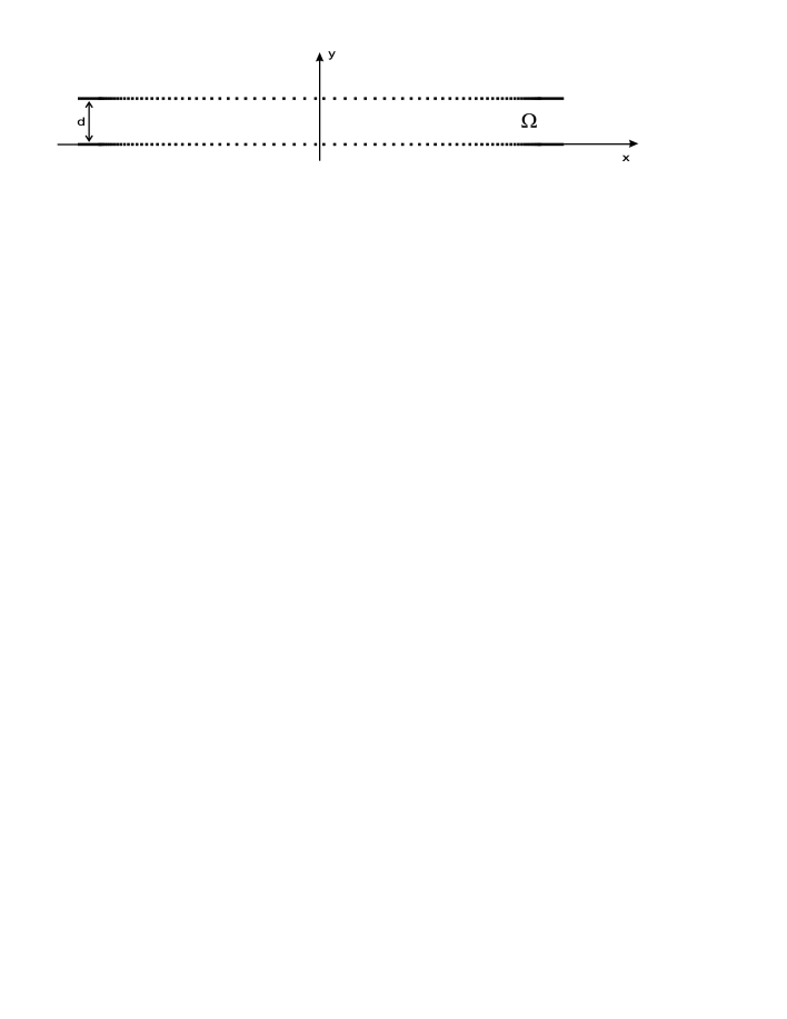
Figure 1: Straight waveguide with Robin boundary conditions. The dotted lines indicate that the boundary-coupling function is allowed to vary.

Putting $\hbar^{2}/2m^{*}=1$ in (1.1), we may identify the particle Hamiltonian with the self-adjoint operator on the Hilbert space $L^{2}(\Omega)$, defined in the following way

$$H_{\alpha}\psi:=-\Delta\psi,\qquad\forall\,\psi\in D(H_{\alpha}):=\left\{\psi\in W^{2,2}(\Omega)\,\big{|}\,\psi\ \mathrm{satisf\/ies}\ \eqref{bc}\right\},$$ (1.3)

where $D(H_{\alpha})$ denotes the domain of the Hamiltonian.

While it is easy to see that $H_{\alpha}$ is symmetric, it is quite difficult to prove that it is self-adjoint. This will be done in the next section. Section 3 is devoted to localization of the essential spectrum and proving the existence of the discrete spectrum. In the final section we study an example numerically to illustrate the spectral properties.

2 The self-adjointness of the Robin Laplacian

For showing the self-adjointness of the Hamiltonian, we were inspired by [5, Section 3]. Our strategy is to show that $H_{\alpha}$ is, in fact, equal to another operator $\tilde{H}_{\alpha}$, which is self-adjoint and defined in following way.

Let us introduce a sesquilinear form

$$h_{\alpha}(\phi,\psi):=\int_{\Omega}\overline{\nabla\phi(x,y)}\cdot\nabla\psi(x,y)\,\mathrm{d}x\,\mathrm{d}y+\int_{\mathbb{R}}\alpha(x)\big{(}\overline{\phi(x,0)}\psi(x,0)+\overline{\phi(x,d)}\psi(x,d)\big{)}\,\mathrm{d}x$$

with the domain

$$D(h_{\alpha}):=W^{1,2}(\Omega).$$

Here the dot denotes the scalar product in $\mathbb{R}^{2}$ and the boundary terms should be understood in the sense of traces [2, Section 4]. We shall denote the corresponding quadratic form by $h_{\alpha}[\psi]:=h_{\alpha}(\psi,\psi)$. In view of the first representation theorem [20, Theorem VI.2.1], there exists the unique self-adjoint operator $\tilde{H}_{\alpha}$ in $L^{2}(\Omega)$ such that $h_{\alpha}(\phi,\psi)=(\phi,\tilde{H}_{\alpha}\psi)$ for all $\psi\in D(\tilde{H}_{\alpha})\subset D(h_{\alpha})$ and $\phi\in D(h_{\alpha})$, where

$$D(\tilde{H}_{\alpha})=\left\{\psi\in D(h_{\alpha})\,\big{|}\,\exists\,F\in L^{2}(\Omega),\forall\,\phi\in D(h_{\alpha}),h_{\alpha}(\phi,\psi)=(\phi,F)\right\}.$$

For showing the equality between $H_{\alpha}$ and $\tilde{H}_{\alpha}$ we will need the following result.

Lemma 2.1.

Let $\alpha\in W^{1,\infty}(\mathbb{R})$ and $\forall\,x\in\mathbb{R}$, $\alpha(x)>0$. For each $F\in L^{2}(\Omega)$, a solution $\psi$ to the problem

$$\forall\,\phi\in W^{1,2}(\Omega),\qquad h_{\alpha}(\phi,\psi)=(\phi,F)$$ (2.1)

belongs to $D(H_{\alpha})$.

Proof 2.2.

For any function $\psi\in W^{1,2}(\Omega)$, we introduce the difference quotient

$$\psi_{\delta}(x,y):=\frac{\psi(x+\delta,y)-\psi(x,y)}{\delta},$$

where $\delta$ is a small real number. Since

$$\left|\psi(x+\delta,y)-\psi(x,y)\right|=\left|\delta\int_{0}^{1}\partial_{x}\psi(x+\delta t,y)\,\mathrm{d}t\right|\leq\left|\delta\right|\int_{0}^{1}\left|\partial_{x}\psi(x+\delta t,y)\right|\,\mathrm{d}t,$$

we get the estimate

$$\int_{\Omega}\left|\psi_{\delta}\right|^{2}\leq\int_{\Omega}\left(\int_{0}^{1}\left|\partial_{x}\psi(x+\delta t,y)\right|\,\mathrm{d}t\right)^{2}\,\mathrm{d}x\,\mathrm{d}y\leq\int_{\Omega}\left(\int_{0}^{1}\left|\partial_{x}\psi(x+\delta t,y)\right|^{2}\,\mathrm{d}t\right)\,\mathrm{d}x\,\mathrm{d}y$$

$$\phantom{\int_{\Omega}\left|\psi_{\delta}\right|^{2}}{}=\int_{0}^{1}\left(\int_{\Omega}\left|\partial_{x}\psi(x+\delta t,y)\right|^{2}\,\mathrm{d}x\,\mathrm{d}y\right)\,\mathrm{d}t=\int_{\Omega}\left|\partial_{x}\psi(x,y)\right|^{2}\,\mathrm{d}x\,\mathrm{d}y.$$

Therefore the inequality

$$\|\psi_{\delta}\|_{L^{2}(\Omega)}\leq\|\psi\|_{W^{1,2}(\Omega)}$$ (2.2)

holds true.

If $\psi$ satisfies (2.1), then $\psi_{\delta}$ is a solution to the problem

$$h_{\alpha}(\phi,\psi_{\delta})=(\phi,F_{\delta})-\int_{\mathbb{R}}\alpha_{\delta}(x)\left(\overline{\phi(x,0)}\psi(x+\delta,0)+\overline{\phi(x,d)}\psi(x+\delta,d)\right)\,\mathrm{d}x,$$

where $\phi\in W^{1,2}(\Omega)$ is arbitrary. Letting $\phi=\psi_{\delta}$ and using the “integration-by-parts” formula for the difference quotients, $(\phi,F_{\delta})=-(\phi_{-\delta},F)$, we get

$$h_{\alpha}[\psi_{\delta}]=-((\psi_{\delta})_{-\delta},F)-\int_{\mathbb{R}}\alpha_{\delta}(x)\left(\overline{\psi_{\delta}(x,0)}\psi(x+\delta,0)+\overline{\psi_{\delta}(x,d)}\psi(x+\delta,d)\right)\,\mathrm{d}x.$$ (2.3)

Using Schwarz inequality, Cauchy inequality, estimate (2.2), boundedness of $\alpha$ and $\alpha_{\delta}$, and embedding of $W^{1,2}(\Omega)$ in $L^{2}(\partial\Omega)$, we can make following estimates

$$\left|((\psi_{\delta})_{-\delta},F)\right|\leq\|F\|_{L^{2}(\Omega)}\|(\psi_{\delta})_{-\delta}\|_{L^{2}(\Omega)}\leq\frac{1}{2}\|F\|_{L^{2}(\Omega)}^{2}+\frac{1}{2}\|\psi_{\delta}\|_{W^{1,2}(\Omega)}^{2},$$

$$\left|\int_{\mathbb{R}}\alpha_{\delta}(x)\left(\overline{\psi_{\delta}(x,0)}\psi(x+\delta,0)+\overline{\psi_{\delta}(x,d)}\psi(x+\delta,d)\right)\,\mathrm{d}x\right|$$

$$\qquad{}\leq C_{1}\|\psi_{\delta}\|_{L^{2}(\partial\Omega)}\|\psi\|_{L^{2}(\partial\Omega)}\leq C_{2}\|\psi_{\delta}\|_{W^{1,2}(\Omega)}\|\psi\|_{W^{1,2}(\Omega)},$$

$$\left|\int_{\mathbb{R}}\alpha(x)\left(|\psi_{\delta}(x,0)|^{2}+|\psi_{\delta}(x,d)|^{2}\right)\,\mathrm{d}x\right|\leq C_{3}\|\psi_{\delta}\|_{L^{2}(\partial\Omega)}^{2}\leq C_{4}\|\psi_{\delta}\|_{W^{1,2}(\Omega)}^{2}$$

with constants $C_{1}$–$C_{4}$ independent of $\delta$. Giving this estimates together, the identity (2.3) yields

$$-\|\psi_{\delta}\|_{W^{1,2}(\Omega)}^{2}\leq C_{4}\|\psi_{\delta}\|_{W^{1,2}(\Omega)}^{2}+C_{2}\|\psi_{\delta}\|_{W^{1,2}(\Omega)}\|\psi\|_{W^{1,2}(\Omega)}+\frac{1}{2}\|F\|_{L^{2}(\Omega)}^{2}+\frac{1}{2}\|\psi_{\delta}\|_{W^{1,2}(\Omega)}^{2}.$$

We get the inequality

$$\|\psi_{\delta}\|_{W^{1,2}(\Omega)}\leq C,$$

where the constant $C$ is independent of $\delta$. This estimate implies

$$\sup_{\delta}\|\psi_{-\delta}\|_{W^{1,2}(\Omega)}<\infty;$$

and, therefore, by [14, § D.4] there exists a function $v\in W^{1,2}(\Omega)$ and a subsequence $\delta_{k}\to 0$ such that $\psi_{-\delta_{k}}\xrightarrow{w}v$ in $W^{1,2}(\Omega)$. But then

$$-\int_{\Omega}\partial_{x}\psi\phi=\int_{\Omega}\psi\partial_{x}\phi=\int_{\Omega}\psi\lim_{\delta_{k}\to 0}\phi_{\delta_{k}}=\lim_{\delta_{k}\to 0}\int_{\Omega}\psi\phi_{\delta_{k}}=-\lim_{\delta_{k}\to 0}\int_{\Omega}\psi_{-\delta}\phi=-\int_{\Omega}v\phi.$$

Thus, $\partial_{x}\psi=v$ in the weak sense, and so $\partial_{x}\psi\in W^{1,2}(\Omega)$. Hence, $\partial_{xx}\psi\in L^{2}(\Omega)$ and $\partial_{xy}\psi\in L^{2}(\Omega)$.

It follows from the standard elliptic regularity theorems (see [14, § 6.3]) that $\psi\in W_{\rm loc}^{2,2}(\Omega)$. Hence, the equation $-\Delta\psi=F$ holds true a.e. in $\Omega$. Thus, $\partial_{yy}\psi=-F-\partial_{xx}\psi\in L^{2}(\Omega)$, and therefore $\psi\in W^{2,2}(\Omega)$.

It remains to check boundary conditions for $\psi$. Using integration by parts, one has

$$(\phi,F)=h_{\alpha}(\psi,\phi)=(\phi,-\Delta\psi)+\int_{\mathbb{R}}\overline{\phi(x,0)}\left[-\partial_{y}\psi(x,0)+\alpha(x)\psi(x,0)\right]\,\mathrm{d}x$$

$$\phantom{(\phi,F)=h_{\alpha}(\psi,\phi)=}{}+\int_{\mathbb{R}}\overline{\phi(x,d)}\left[\partial_{y}\psi(x,d)+\alpha(x)\psi(x,d)\right]\,\mathrm{d}x$$

for any $\phi\in W^{1,2}(\Omega)$. This implies the boundary conditions because $-\Delta\psi=F$ a.e. in $\Omega$ and $\phi$ is arbitrary.

Theorem 2.3.

Let $\alpha\in W^{1,\infty}(\mathbb{R})$ and $\forall\,x\in\mathbb{R},\ \alpha(x)>0$. Then $\tilde{H}_{\alpha}=H_{\alpha}$.

Proof 2.4.

Let $\psi\in D(H_{\alpha})$, i.e., $\psi\in W^{2,2}(\Omega)$ and $\psi$ satisfies the boundary conditions (1.2). Then $\psi\in D(h_{\alpha})=W^{1,2}(\Omega)$ and by integration by parts and (1.2) we get for all $\phi\in D(h_{\alpha})$ the relation

$$h_{\alpha}(\phi,\psi)=\int_{\mathbb{R}}\overline{\phi(x,d)}\partial_{y}\psi(x,d)\,\mathrm{d}x-\int_{\mathbb{R}}\overline{\phi(x,0)}\partial_{y}\psi(x,0)\,\mathrm{d}x-\int_{\Omega}\overline{\phi(x,y)}\Delta\psi(x,y)\,\mathrm{d}x\,\mathrm{d}y$$

$$\phantom{h_{\alpha}(\phi,\psi)=}{}+\int_{\mathbb{R}}\alpha(x)\overline{\phi(x,d)}\psi(x,d)\,\mathrm{d}x+\int_{\mathbb{R}}\alpha(x)\overline{\phi(x,0)}\psi(x,0)\,\mathrm{d}x$$

$$\phantom{h_{\alpha}(\phi,\psi)}{}=-\int_{\Omega}\overline{\phi(x,y)}\Delta\psi(x,y)\,\mathrm{d}x\,\mathrm{d}y.$$

It means that there exists $\eta:=-\Delta\psi\in L^{2}(\Omega)$ such that $\forall\,\phi\in D(h_{\alpha})$, $h_{\alpha}(\phi,\psi)=(\phi,\eta)$. That is, $\tilde{H}_{\alpha}$ is an extension of $H_{\alpha}$.

The other inclusion holds as a direct consequence of Lemma 2.1 and the first representation theorem.

3 The spectrum of Hamiltonian

In this section we will investigate the spectrum of the Hamiltonian with respect to the behavior of the function $\alpha$. In whole section we suppose that $\alpha\in W^{1,\infty}(\mathbb{R})$ and $\forall\,x\in\mathbb{R}$, $\alpha(x)>0$. We start with the simplest case.

3.1 Unperturbed system

If $\alpha(x)=\alpha_{0}>0$ is a constant function, the Schrödinger equation can be easily solved by separation of variables. The spectrum of the Hamiltonian is then $\sigma(H_{\alpha_{0}})=[E_{1}(\alpha_{0}),\infty)$, where $E_{1}(\alpha_{0})$ is the first transversal eigenvalue. The transversal eigenfunctions have the form

$$\chi_{n}(y;\alpha)=N_{\alpha}\left(\frac{\alpha}{\sqrt{E_{n}(\alpha)}}\sin\left(\sqrt{E_{n}(\alpha)}y\right)+\cos\left(\sqrt{E_{n}(\alpha)}y\right)\right),$$ (3.1)

where $N_{\alpha}$ is a normalization constant and the eigenvalues $E_{n}(\alpha)$ are determined by the implicit equation

$$f(E_{n};\alpha)=2\alpha\sqrt{E_{n}(\alpha)}\cos(\sqrt{E_{n}(\alpha)}d)+(\alpha^{2}-E_{n}(\alpha))\sin(\sqrt{E_{n}(\alpha)}d)=0.$$

Note that there are no eigenvalues below the bottom of the essential spectrum, i.e., $\sigma_{\rm disc}=\varnothing$.

3.2 The stability of essential spectrum

As we have seen, if $\alpha$ is a constant function, the essential spectrum of the Hamiltonian is the interval $[E_{1}(\alpha_{0}),\infty)$. Now we prove that the same spectral result holds if $\alpha$ tends to $\alpha_{0}$ at infinity.

Theorem 3.1.

If $\lim\limits_{|x|\to\infty}\alpha(x)-\alpha_{0}=0$ then $\sigma_{\rm ess}(H_{\alpha})=[E_{1}(\alpha_{0}),\infty)$.

The proof of this theorem is achieved in two steps. Firstly, in Lemma 3.3, we employ a Neumann bracketing argument to show that the threshold of essential spectrum does not descent below the energy $E_{1}(\alpha_{0})$. Secondly, in Lemma 3.5, we prove that all values above $E_{1}(\alpha_{0})$ belongs to the essential spectrum by means of the following characterization of the essential spectrum which we have adopted from [9].

Lemma 3.2.

Let $H$ be a non-negative self-adjoint operator in a complex Hilbert space $\mathcal{H}$ and $h$ be the associated quadratic form. Then $\lambda\in\sigma_{\rm ess}(H)$ if and only if there exists a sequence $\{\psi_{n}\}_{n=1}^{\infty}\subset D(h)$ such that

1. $\forall\,n\in\mathbb{N}\setminus\{0\}$, $\|\psi_{n}\|=1$,

2. $\psi_{n}\xrightarrow[n\to\infty]{w}0\ \mathrm{in}\ \mathcal{H}$,

3. $(H-\lambda)\psi_{n}\xrightarrow[n\to\infty]{}0\ \mathrm{in}\ D(h)^{*}$.

Here $D(h)^{*}$ denotes the dual of the space $D(h)$. We note that

$$\|\psi\|_{D(h)^{*}}=\sup_{\phi\in D(h)\setminus\{0\}}\frac{|(\phi,\psi)|}{\|\phi\|_{1}}$$

with

$$\|\phi\|_{1}:=\sqrt{h[\phi]+\|\phi\|^{2}}.$$

The main advantage of Lemma 3.2 is that it requires to find a sequence from the form domain of $H$ only, and not from $D(H)$ as it is required by the Weyl criterion [8, Lemma 4.1.2]. Moreover, in order to check the limit from (iii), it is still sufficient to consider the operator $H$ in the form sense, i.e. we will not need to assume that $\alpha$ is differentiable in our case.

Lemma 3.3.

If $\lim\limits_{|x|\to\infty}\alpha(x)-\alpha_{0}=0$ then $\inf\sigma_{\rm ess}(H_{\alpha})\geq E_{1}(\alpha_{0})$.

Proof 3.4.

Since $\alpha(x)-\alpha_{0}$ vanishes at infinity, for any fixed $\varepsilon>0$ there exists $a>0$ such that

$$|x|>a\ \Rightarrow\ |\alpha(x)-\alpha_{0}|<\varepsilon.$$ (3.2)

Cutting $\Omega$ by additional Neumann boundary parallel to the $y$-axis at $x=\pm a$, we get new operator $H_{\alpha}^{(N)}$ defined using quadratic form. We can decompose this operator $H_{\alpha}^{(N)}=H_{\alpha,t}^{(N)}\oplus H_{\alpha,c}^{(N)},$ where the “tail” part corresponds to the two halfstrips ($|x|>a$) and the rest to the central part with the Neumann condition on the vertical boundary. Using Neumann bracketing, cf. [26, Section XIII.15], we get $H_{\alpha}^{(N)}\leq H_{\alpha}$ in the sense of quadratic forms.

We denote $\alpha_{\min}(a):=\inf\limits_{|x|>a}\alpha(x).$ Since $\sigma_{\rm ess}(H_{\alpha_{\min},t}^{(N)})=[E_{1}(\alpha_{\min}),\infty)$ and $H_{\alpha_{\min},t}^{(N)}\leq H_{\alpha,t}^{(N)}$ in the sense of quadratic forms, we get the following estimate of the bottom of the essential spectrum of the “tail” part

$$E_{1}(\alpha_{\min})\leq\inf\sigma_{\rm ess}(H_{\alpha,t}^{(N)}).$$ (3.3)

Since the spectrum of $H_{\alpha,c}^{(N)}$ is purely discrete, cf. [8, Chapter 7], the minimax principle gives the inequality

$$\inf\sigma_{\rm ess}(H_{\alpha,t}^{(N)})\leq\inf\sigma_{\rm ess}(H_{\alpha}).$$ (3.4)

Since the assertion (3.2) yields $\alpha_{0}-\varepsilon<\alpha_{\min}$ and $E_{1}$ is an increasing function of $\alpha$, we have

$$E_{1}(\alpha_{0}-\varepsilon)<E_{1}(\alpha_{\min}).$$ (3.5)

Giving together (3.3), (3.4), and (3.5) we get the relation $E_{1}(\alpha_{0}-\varepsilon)<\inf\sigma_{\rm ess}(H_{\alpha}).$ The claim then follows from the fact that $E_{1}=E_{1}(\alpha)$ is a continuous function.

Lemma 3.5.

If $\lim\limits_{|x|\to\infty}\alpha(x)-\alpha_{0}=0$ then $[E_{1}(\alpha_{0}),\infty)\subseteq\sigma_{\rm ess}(H_{\alpha})$.

Proof 3.6.

Let $\lambda\in[E_{1}(\alpha_{0}),\infty)$. We shall construct a sequence $\left\{\psi_{n}\right\}_{n=1}^{\infty}$ satisfying the assumptions (i)–(iii) of Lemma 3.2. We define the following family of functions

$$\psi_{n}(x,y):=\varphi_{n}(x)\chi_{1}(y;\alpha_{0})\exp\left(i\sqrt{\lambda-E_{1}(\alpha_{0})}x\right),$$

where $\chi_{1}$ is the lowest transversal function (3.1) and $\varphi_{n}(x):=n^{-1/2}\varphi(x/n-n)$ with $\varphi$ satisfying

1. $\varphi\in C_{0}^{\infty}(\mathbb{R})$,

2. $\forall\,x\in\mathbb{R}$, $0\leq\varphi(x)\leq 1$,

3. $\forall\,x\in\left(-1/4,1/4\right)$, $\varphi=1$,

4. $\forall\,x\in\mathbb{R}\setminus\left[-1/4,1/4\right]$, $\varphi=0$,

5. $\|\varphi\|_{L^{2}(\mathbb{R})}=1$.

Note that $\mathrm{supp}\ \varphi_{n}\subset(n^{2}-n,n^{2}+n)$. It is clear that $\psi_{n}$ belongs to the form domain of $H_{\alpha}$. The assumption (i) of Lemma 3.2 is satisfied due to the normalization of $\chi_{1}$ and $\varphi$.

The point (ii) of Lemma 3.2 requires that $(\phi,\psi_{n})\to 0$ as $n\to\infty$ for all $\phi\in C_{0}^{\infty}(\Omega)$, a dense subset of $L^{2}(\Omega)$. However, it follows at once because $\phi$ and $\psi_{n}$ have disjoint supports for $n$ large enough.

Hence, it remains to check that $\|(H_{\alpha}-\lambda)\psi_{n}\|_{D(h)^{*}}\to 0$ as $n\to\infty$. An explicit calculation using integration by parts, boundary conditions (1.2) and the relations

$$\|\dot{\varphi}_{n}\|_{L^{2}(\mathbb{R})}=n^{-1}\|\dot{\varphi}\|_{L^{2}(\mathbb{R})},\qquad\|\ddot{\varphi}_{n}\|_{L^{2}(\mathbb{R})}=n^{-2}\|\ddot{\varphi}\|_{L^{2}(\mathbb{R})}$$ (3.6)

yields

$$\big{|}\big{(}\phi,(H_{\alpha}-\lambda)\psi_{n}\big{)}\big{|}=\bigg{|}\int_{\Omega}\overline{\phi(x,y)}\chi_{1}(y;\alpha_{0})\ddot{\varphi}_{n}(x)\exp\left(i\sqrt{\lambda-E_{1}(\alpha_{0})}x\right)\,\mathrm{d}x\,\mathrm{d}y$$

$$\qquad{}+2i\int_{\Omega}\overline{\phi(x,y)}\chi_{1}(y;\alpha_{0})\dot{\varphi}_{n}(x)\sqrt{\lambda-E_{1}(\alpha_{0})}\exp\left(i\sqrt{\lambda-E_{1}(\alpha_{0})}x\right)\,\mathrm{d}x\,\mathrm{d}y\bigg{|}$$

$$\qquad{}\leq n^{-2}\|\phi\|_{L^{2}(\Omega)}\|\chi_{1}\|_{L^{2}((0,d))}\|\ddot{\varphi}\|_{L^{2}(\mathbb{R})}+2n^{-1}\|\phi\sqrt{\lambda{-}E_{1}(\alpha_{0})}\|_{L^{2}(\Omega)}\|\chi_{1}\|_{L^{2}((0,d))}\|\dot{\varphi}\|_{L^{2}(\mathbb{R})}$$

for all $\phi\in D(h_{\alpha})$. The claim then follows from the fact that both terms at the r.h.s. go to zero as $n\to\infty$.

3.3 The existence of bound states

Now we show that if $\alpha-\alpha_{0}$ vanishes at infinity, some behavior of the function $\alpha$ may produce a non-trivial spectrum below the energy $E_{1}(\alpha_{0})$. Note that this together with the assumption of Theorem 3.1 implies that the spectrum below $E_{1}(\alpha_{0})$ consists of isolated eigenvalues of finite multiplicity, i.e. $\sigma_{\rm disc}(H_{\alpha})\neq\varnothing$. Sufficient condition that pushes the spectrum of the Hamiltonian below $E_{1}(\alpha_{0})$ is introduced in the following theorem.

Theorem 3.7.

Suppose

1. $\alpha(x)-\alpha_{0}\in L^{1}(\mathbb{R})$,

2. $\int_{\mathbb{R}}\left(\alpha(x)-\alpha_{0}\right)\,\mathrm{d}x<0$.

Then $\inf\sigma(H_{\alpha})<E_{1}(\alpha_{0})$.

Proof 3.8.

The proof is based on the variational strategy of finding a trial function $\psi$ from the form domain of $H_{\alpha}$ such that

$$Q_{\alpha}[\psi]:=h_{\alpha}[\psi]-E_{1}(\alpha_{0})\|\psi\|_{L^{2}(\Omega)}^{2}<0.$$ (3.7)

Inspired by [19], we define a sequence

$$\psi_{n}(x,y):=\varphi_{n}(x)\chi_{1}(y;\alpha_{0}),\qquad\varphi_{n}(x):=n^{-1/2}\varphi(x/n),$$

where the function $\varphi$ was defined in the proof of Lemma 3.5. Using the relations (3.6) and the integration by parts we get

$$Q_{\alpha}[\psi_{n}]=n^{-2}\|\dot{\varphi}\|_{L^{2}(\mathbb{R})}^{2}+\left(|\chi_{1}(0;\alpha_{0})|^{2}+|\chi_{1}(d;\alpha_{0})|^{2}\right)\int_{\mathbb{R}}(\alpha(x)-\alpha_{0})\varphi_{n}(x)\,\mathrm{d}x.$$

Since the integrand is dominated by the $L^{1}$-norm of $\alpha-\alpha_{0}$ we have the limit

$$\lim_{n\to\infty}Q_{\alpha}[\psi_{n}]=\left(|\chi_{1}(0;\alpha_{0})|^{2}+|\chi_{1}(d;\alpha_{0})|^{2}\right)\int_{\mathbb{R}}(\alpha(x)-\alpha_{0})\,\mathrm{d}x$$

by dominated convergence theorem. This expression is negative according to the assumptions. Now, it is enough to take $n$ sufficiently large to satisfy inequality (3.7).

4 A ‘rectangular well’ example

To illustrate the above results and to understand the behavior of the spectrum of the Hamiltonian in more detail, we shall now investigate an example. Inspired by [15] we choose the function $\alpha$ to be a steplike function which makes it possible to solve the corresponding Schrödinger equation numerically by employing the mode-matching method. The simplest non-trivial case concerns a ‘rectangular well’ of a width $2a$,

$$\alpha(x)=\left\{\begin{array}[]{ll}\alpha_{1}&\mathrm{if}\ |x|<a,\vspace{1mm}\\ \alpha_{0}&\mathrm{if}\ |x|\geq a\end{array}\right.$$

with $a>0$ and $0<\alpha_{1}<\alpha_{0}$. In view of Theorem 3.7 this waveguide system has bound states. In particular, one expects that in the case when $\alpha_{1}$ is close to zero and $\alpha_{0}$ is large the spectral properties will be similar to those of the situation studied in [10].

Since the system is symmetric with respect to the $y$-axis, we can restrict ourselves to the part of $\Omega$ in the first quadrant and we may consider separately the symmetric and antisymmetric solutions, i.e. to analyze the halfstrip with the Neumann or Dirichlet boundary condition at the segment $(0,d)$ on $y$-axis, respectively.

4.1 Preliminaries

Theorem 3.1 enables us to localize the essential spectrum in the present situation, i.e., $\sigma_{\rm ess}(H_{\alpha})=[E_{1}(\alpha_{0}),\infty)$. Moreover, according to the minimax principle we know that isolated eigenvalues of $H_{\alpha}$ are squeezed between those of $H_{a,c}^{(N)}$ and $H_{a,c}^{(D)}$, the Hamiltonians in the central part with Neumann or Dirichlet condition on the vertical boundary, respectively. The Neumann estimate tells us that $\inf\sigma(H_{\alpha})\geq E_{1}(\alpha_{1})$. One finds that the $n$-th eigenvalue $E_{n}$ of $H_{\alpha}$ is estimated by

$$E_{1}(\alpha_{1})+\left(\frac{(n-1)\pi}{2a}\right)^{2}\leq E_{n}\leq E_{1}(\alpha_{1})+\left(\frac{n\pi}{2a}\right)^{2}.$$

4.2 Mode-matching method

Let us pass to the mode-matching method. A natural Ansatz for the solution of an energy $\lambda\in(E_{1}(\alpha_{1}),E_{1}(\alpha_{0}))$ is

$$\psi_{s/a}(x,y)=\sum_{n=1}^{\infty}a_{n}^{s/a}\left\{\begin{array}[]{c}\frac{\cosh(l_{n}x)}{\cosh(l_{n}a)}\vspace{2mm}\\ \frac{\sinh(l_{n}x)}{\sinh(l_{n}a)}\end{array}\right\}\chi_{n}(y;\alpha_{1})\qquad\mathrm{for}\ 0\leq x<a,$$

$$\psi_{s/a}(x,y)=\sum_{n=1}^{\infty}b_{n}^{s/a}\exp(-k_{n}(x-a))\chi_{n}(y;\alpha_{0})\qquad\mathrm{for}\ x\geq a,$$

where the subscripts and superscripts $s$, $a$ distinguish the symmetric and antisymmetric case, respectively. The longitudinal momenta are defined by

$$l_{n}:=\sqrt{E_{n}(\alpha_{1})-\lambda},\qquad k_{n}:=\sqrt{E_{n}(\alpha_{0})-\lambda}.$$

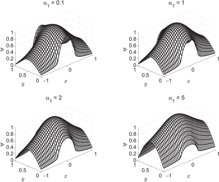
Figure 2: Ground state eigenfunctions for $a/d=0.3$, $\alpha_{0}=20$.

As an element of the domain (1.3), the function $\psi$ should be continuous together with its normal derivative at the segment dividing the two regions, $x=a$. Using the orthonormality of $\{\chi_{n}\}$ we get from the requirement of continuity

$$\sum_{n=1}^{\infty}a_{n}\int_{0}^{d}\chi_{n}(y,\alpha_{1})\chi_{m}(y;\alpha_{0})\,\mathrm{d}y=b_{m}.$$ (4.1)

In the same way, the normal-derivative continuity at $x=a$ yields

$$\sum_{n=1}^{\infty}a_{n}l_{n}\left\{\begin{array}[]{c}\tanh\\ \coth\end{array}\right\}(l_{n}a)\int_{0}^{d}\chi_{n}(y;\alpha_{1})\chi_{m}(y;\alpha_{0})\,\mathrm{d}y+b_{m}k_{m}=0.$$ (4.4)

Substituting (4.1) to (4.4) we can write the equation as

$$\mathbf{Ca}=\mathbf{0},$$ (4.5)

where

$$C_{mn}=\left(l_{n}\left\{\begin{array}[]{c}\tanh\\ \coth\end{array}\right\}(l_{n}a)+k_{m}\right)\int_{0}^{d}\chi_{n}(y;\alpha_{1})\chi_{m}(y;\alpha_{0})\,\mathrm{d}y.$$

In this way we have transformed a partial-differential-equation problem to a solution of an infinite system of linear equations. The latter will be solved numerically by using in (4.5) an $N$ by $N$ subblock of $\mathbf{C}$ with large $N$.

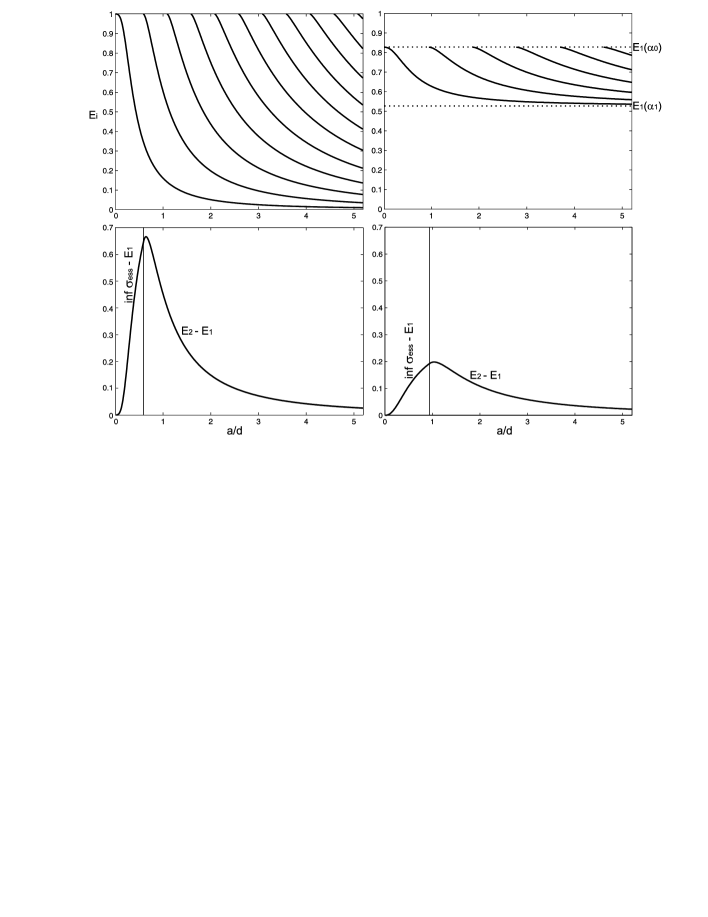
Figure 3: The dependence of eigenvalues (in the units of $(\pi/d)^{2}$) on $a/d$ in the case $\alpha_{0}=10^{5}$, $\alpha_{1}=10^{-5}$ (left) and $\alpha_{0}=20$, $\alpha_{1}=5$ (right) and corresponding first gaps.

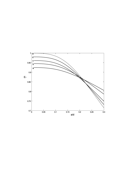
Figure 4: The dependence of first eigenvalue (in the units of $(\pi/d)^{2}$) on $a/d$ in the cases: (a) $\alpha_{0}=50,\alpha_{1}=3$, (b) $\alpha_{0}=70,\alpha_{1}=2$, (c) $\alpha_{0}=100,\alpha_{1}=1$, (d) $\alpha_{0}=200,\alpha_{1}=0.5$, and in the Dirichlet–Neumann case (e) adopted from [10].

4.3 Numerical results

The dependence of the ground state wavefunction with respect to $\alpha_{1}$ for the central part of the halfwidth $a/d=0.3$ is illustrated in Fig. 2. The slope of the wavefunctions at the boundary between different $\alpha_{i}$ becomes smoother with increasing $\alpha_{1}$, at $\alpha_{1}$ approaching $\alpha_{0}$ the wavefunction is spread further and further in the $x$-direction, and at $\alpha_{1}=\alpha_{0}$ bound state disappears.

Fig. 3 shows the bound-state energies as functions of the ‘window’ halfwidth $a/d$ in the case $\alpha_{0}=10^{5}$, $\alpha_{1}=10^{-5}$ (on the left) and $\alpha_{0}=20$, $\alpha_{1}=5$ (on the right). We see that the energies (in both cases) decrease monotonously with the increasing ‘window’ width and in the limit approach the uniform value $E_{1}(\alpha_{1})$. Their number increases as a function of $a/d$. Comparing this figure with Fig. 4 in [23] or Fig. 5 in [25], where the authors study the planar waveguide comprised of two straight regions connected by a region of constant curvature (with Dirichlet or mixed boundary conditions, respectively), we may see the similar behavior of the eigenvalues below the fundamental propagation constant. This comparison shows a community of the physical processes taking place in different structures where the longitudinal uniformity of the waveguide is broken by some obstacle – either by the different boundary conditions or the bend. For illustration, the first gap, i.e., the difference between first and second eigenvalue (or between first eigenvalue and the bottom of the essential spectrum if there is only one eigenvalue), is plotted in the bottom part of Fig. 3. It is interesting that the dependence on $a/d$ in the region where more than one eigenvalue exists is not monotonous, but there is a maximum.

We can compare the dependence of the first eigenvalue on $a/d$ with the system studied in [10]. The authors there are interested in the model of straight quantum waveguide with combined Dirichlet and Neumann boundary conditions. Fig. 4 shows that the larger $\alpha_{0}$ and the smaller $\alpha_{1}$ is (curves $a$, $b$, $c$, and $d$), the closer to the Dirichlet–Neumann case (curve $e$) is the behavior of the first eigenvalue as a function of $a/d$.

Acknowledgements

The author thanks the referees for helpful suggestions.

References

- [1]
- [2] Adams R.A., Sobolev spaces, Academic Press, New York, 1975.
- [3] Bendali A., Lemrabet K., The effect of a thin coating on the scattering of a time-harmonic wave for the Helmholtz equation, SIAM J. Appl. Math. 56 (1996), 1664–1693.
- [4] Borisov D., Exner P., Gadyl’shin R., Krejčiřík D., Bound states in weakly deformed strips and layers, Ann. Henri Poincaré 2 (2001), 553–572, math-ph/0011052.
- [5] Borisov D., Krejčiřík D., PT-symmetric waveguide, arXiv:0707.3039.
- [6] Bulla W., Gesztesy F., Renger W., Simon B., Weakly coupled boundstates in quantum waveguides, Proc. Amer. Math. Soc. 127 (1997), 1487–1495.
- [7] Chenaud B., Duclos P., Freitas P., Krejčiřík D., Geometrically induced discrete spectrum in curved tubes, Differential Geom. Appl. 23 (2005), 95–105, math.SP/0412132.
- [8] Davies E.B., Spectral theory and differential operators, Camb. Univ. Press, Cambridge, 1995.
- [9] Dermenjian Y., Durand M., Iftimie V., Spectral analysis of an acoustic multistratified perturbed cylinder, Comm. Partial Differential Equations 23 (1998), 141–169.
- [10] Dittrich J., Kříž J., Bound states in straight quantum waveguides with combined boundary conditions, J. Math. Phys. 43 (2002) 3892–3915, math-ph/0112018.
- [11] Dittrich J., Kříž J., Curved planar quantum wires with Dirichlet and Neumann boundary conditions, J. Phys. A: Math. Gen. 35 (2002), L269–L275, math-ph/0203007.
- [12] Duclos P., Exner P., Curvature-induced bound states in quantum waveguides in two and three dimensions, Rev. Math. Phys. 7 (1995), 73–102.
- [13] Engquist B., Nedelec J.C., Effective boundary conditions for electro-magnetic scattering in thin layers, Rapport Interne, Vol. 278, CMAP, 1993.
- [14] Evans L.C., Partial differential equations, American Mathematical Society, Providence, 1998.
- [15] Exner P., Krejčiřík D., Quantum waveguides with a lateral semitransparent barrier: spectral and scattering properties, J. Phys. A: Math. Gen. 32 (1999), 4475–4494, cond-mat/9904379.
- [16] Exner P., Šeba P., Bound states in curved quantum waveguides, J. Math. Phys. 30 (1989), 2574–2580.
- [17] Exner P., Šeba P., Tater M., Vaněk D., Bound states and scattering in quantum waveguides coupled laterally through a boundary window, J. Math. Phys. 37 (1996), 4867–4887, cond-mat/9512088.
- [18] Freitas P., Krejčiřík D., Waveguides with combined Dirichlet and Robin boundary conditions, Math. Phys. Anal. Geom. 9 (2006), 335–352, math-ph/0701075.
- [19] Goldstone J., Jaffe R.L., Bound states in twisting tubes, Phys. Rev. B 45 (1992), 14100–14107.
- [20] Kato T., Perturbation theory for linear operators, Springer-Verlag, Berlin, 1966.
- [21] Kovařík H., Krejčiřík D., A Hardy inequality in a twisted Dirichlet–Neumann waveguide, Math. Nachr., to appear, math-ph/0603076.
- [22] Krejčiřík D., Kříž J., On the spectrum of curved planar waveguides, Publ. RIMS Kyoto Univ. 41 (2005), 757–791.
- [23] Lin K., Jaffe R.L., Bound states and quantum resonances in quantum wires with circular bends, Phys. Rev. B 54 (1996), 5750–5762.
- [24] Londergan J.T., Carini J.P., Murdock D.P., Binding and scattering in two-dimensional systems, Lect. Note in Phys., Vol. 60, Springer, Berlin, 1999.
- [25] Olendski O., Mikhailovska L., Localized-mode evolution in a curved planar waveguide with combined Dirichlet and Neumann boundary conditions, Phys. Rev. E 67 (2003), 056625, 11 pages.
- [26] Reed M., Simon B., Methods of modern mathematical physics. IV. Analysis of operators, Academic Press, New York, 1978.