Random bistochastic matrices
Abstract
Ensembles of random stochastic and bistochastic matrices are investigated.
While all columns of a random stochastic matrix can be chosen independently,
the rows and columns of a bistochastic matrix have to be correlated.
We evaluate the probability measure induced into the Birkhoff polytope
of bistochastic matrices by applying the Sinkhorn algorithm to
a given ensemble of random stochastic matrices.
For matrices of order we derive explicit formulae
for the probability distributions induced by random stochastic
matrices with columns distributed according to the Dirichlet distribution.
For arbitrary we construct an initial ensemble of stochastic matrices which allows one to generate
random bistochastic matrices according to a distribution locally flat at the center of the Birkhoff polytope.
The value of the probability density at this point enables us to obtain an estimation of the volume of the
Birkhoff polytope, consistent with recent asymptotic results.
PACS numbers: 02.10.Yn, 02.30.Cj, 05.10.-a
Mathematics Subject Classification: 15A51, 15A52, 28C99
e-mails: valerio@ictp.it h.j.sommers@uni-due.de w.bruzda@uj.edu.pl karol@cft.edu.pl
1 Introduction
A stochastic matrix is defined as a square matrix of size , consisting of non–negative elements, such that the sum in each column is equal to unity. Such matrices provide an important tool often applied in various fields of theoretical physics, since they represent Markov chains. In other words, any stochastic matrix maps the set of probability vectors into itself. Weak positivity of each element of guarantees that the image vector does not contain any negative components, while the probability is preserved due to the normalization of each column of .
A stochastic matrix is called bistochastic (or doubly stochastic) if additionally each of its rows sums up to unity, so that the map preserves identity and for this reason it is given the name unital. Bistochastic matrices are used in the theory of majorization [1, 2, 3] and emerge in several physical problems [4]. For instance they may represent a transfer process at an oriented graph consisting of nodes.
The set of bistochastic matrices of size can be viewed as a convex polyhedron in . Due to the Birkhoff theorem, any bistochastic matrix can be represented as a convex combination of permutation matrices. This dimensional set is often called Birkhoff polytope. Its volume with respect to the Euclidean measure is known [5, 6, 7] for .
To generate a random stochastic matrix one may take an arbitrary square matrix with non-negative elements and renormalize each of its columns. Alternatively, one may generate independently each column according to a given probability distribution defined on the probability simplex. A standard choice is the Dirichlet distribution (14), which depends on the real parameter and interpolates between the uniform measure obtained for and the statistical measure for — see e.g. [8].
Random bistochastic matrices are more difficult to generate, since the constraints imposed for the sums in each column and each row imply inevitable correlations between elements of the entire matrix. In order to obtain a bistochastic matrix one needs to normalize all its rows and columns, and this cannot be performed independently. However, since the both sets of stochastic and unital matrices are convex, iterating such a procedure, converges [9] and yields a bistochastic matrix. Note that initializing the scheme of alternating projections with different ensembles of initial conditions leads to various probability measures on the set.
The aim of this work is to analyze probability measures inside the Birkhoff polytope. In particular we discuss methods of generating random bistochastic matrices according to the uniform (flat) measure in this set. Note that the brute force method of generating random points distributed uniformly inside the unit cube of dimension and checking if the bistochasticity conditions are satisfied, is not effective even for of order of , since the volume of the Birkhoff polytope decreases fast with the matrix size.
The paper is organized as follows. In Section 2 we present after Sinkhorn [10] two equivalent algorithms producing a bistochastic matrix out of any square matrix of non-negative elements. An implicit formula (13) expressing the probability distribution in the set of bistochastic matrices for arbitrary is derived in Sec. 3.1, while exact formulas for the case are presented in Section 3.2. Furthermore, we obtain its power series expansion around the center of the Birkhoff polytope and for each we single out a particular initial distribution in the set of stochastic matrices, such that the output distribution is flat (at least locally) in the vicinity of . Finally, in section 5 we compute the value of the probability density at this very point and obtain an estimation of the volume of the set of bistochastic matrices, consistent with recent results of Canfield and McKay [12]. In Appendix A we demonstrate equivalence of two algorithms used to generate random bistochastic matrices. The key expression of this paper (36) characterising the probability distribution for random bistochastic matrices in vicinity of the center of the Birkhoff polytope is derived in Appendix B, while the third order expansion is worked out in Appendix C.
2 How to generate a bistochastic matrix?
2.1 Algorithm useful for numerical computation
In 1964 Sinkhorn [10] introduced the following iterative algorithm leading to a bistochastic matrix, based on alternating normalization of rows and columns of a given square matrix with non-negative entries:
Algorithm 1 (rows/columns normalization)
- 1)
take an input stochastic matrix such that each row contains at least one positive element,
- 2)
normalize each row-vector of by dividing it by the sum of its elements,
- 3)
normalize each column-vector as in the previous point 2),
- 4)
stop if the matrix is bistochastic up to certain accuracy in some norm , otherwise go to point 2) .
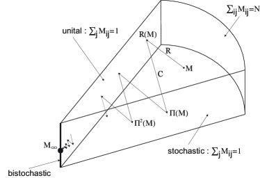
The above algorithm is symbolically visualized in Fig. 1. For an initial point one may take an arbitrary matrix with non-negative entries. To fix the scale we may assume that the sum of all entries is equal to , so belongs to interior of the dimensional simplex . The transformation of normalization of the rows of produces a unital matrix, for which the sum of all (non-negative) entries in each row is equal to unity. Subsequent normalization of the columns of maps this matrix into the set of stochastic matrices. This step can be rewritten as , where denotes the transposition of the matrix. Hence the entire map reads For instance if in the limit we aim to get a bistochastic matrix
| (1) |
Since both these sets are convex, our procedure can be considered as a particular example of a general construction called ’projections on convex sets’. Due to convexity of these sets the procedure of alternating projections converges to a point belonging to the intersection of both sets [9]. An analogous method was recently used by Audenaert and Scheel to generate quantum bistochastic maps [13].
2.2 Algorithm suitable for analytical calculation
To perform analytical calculations of probability distribution inside the Birkhoff polytope we are going to use yet another algorithm to generate bistochastic matrix, the idea of which is due to Djoković [14]. Already in his earlier paper [10] Sinkhorn demonstrated that for a given positive matrix there exists exactly one doubly stochastic matrix such that . In order to extend such important result from posistive matrices to non-negative ones, one has to introduce the hypotesis of fully indecomposability [11, 14]. For the sake of clarity and reading, we prefer to mention here that the set of non-fully indecomposable (stochastic) matrices constitute a zero measure set within the set of all stochastic matrices, instead of going through the details of Sinkhorn’s proof. This means that the converge of our algorithms we will assume to hold true from now onwards, has to be intended almost everywhere in the compact set of stochastic matrices, with respect to the usual Lebesgue measure.
Here and denote diagonal matrices with positive entries determined uniquely up to a scalar factor.
To set the notation, we will denote with the positive semi-axis whereas, the symbol will be used for . Let us now consider the positive cone and the set of endomorphisms over it, , representable by means of matrices consisting of non negative elements . For any given two vectors and in , one can consider a map , given by
| (2a) | ||||
| (2b) | ||||
Defining the positive diagonal matrices , and respectively, one can observe that . Our purpose is to design an algorithm that takes a generic as an input and produces as an output an appropriate pair of vectors such that is bistochastic.
The stochasticity condition implies
| (3a) | |||
| Analogously, unitality implies | |||
| (3b) | |||
so that . Both equations (3) can be merged together into a single equation for ,
| (4) |
which can be interpreted as a kind of equation of the motion for , as it corresponds to a stationary solution of the action–like functional
| (5) |
Equations (4–5) imply that if is a solution, then for any the rescaled vector is as well a solution of (5). Thus we may fix and try to solve (4) for . Differentiating eq. (5) we get
| (6) |
is a stochastic matrix. Since , unitality of is attained once we impose stationarity to (6). Hence the stationary implies that becomes bistochastic. Equation (5) displays convexity of for very small . The function is convex at the stationary point and starts to become concave for large . Thus there is a unique minimum of the function which can be reached by the following iteration procedure:
| (7) |
where we fix and iterate the remaining components only. We start with setting which leads to
Algorithm 2 (convergent sequences of vectors)
- 1)
take an input stochastic matrix and define the vector ,
- 2)
run equation (7) yielding the vector out of ,
- 3)
stop if the matrix is bistochastic up to a certain accuracy in some norm , otherwise go to point 2).
The Algorithm (1) is expected to converge faster than the Algorithm (2), so it can be recommended for numerical implementation. On the other hand Algorithm (2) is useful to evaluate analytically the probability measure induced into the Birkhoff polytope by a given choice of the input ensemble, and it is used for this purpose in further sections. The equivalence of these two algorithms is shown in Appendix A.
3 Probability measures in the Birkhoff polytope
Assume that the algorithm is initiated with a random matrix drawn according to a given distribution of matrices of non negative elements . We want to know the distribution of the resulting bistochastic matrices obtained as output of the Algorithm (2). To this end, using eq. (4) and imposing stationarity condition (6), we write the distribution for by integrating over delta functions
| (8) |
where the Jacobian factor reads
| (9) |
Here and in the following will indicate the block matrix , that is positive defined, and the symbol will denote the probability density of matrices . This notation will also be used for matrices whose elements are functions of elements of another matrix, namely . Plugging eq. (9) into (8) and introducing again the delta functions for variables of (3a) we obtain
| (10) | ||||
| Using the property of the Dirac delta function and making use of the Heaviside step function , we perform integration over the variables . Introducing new variables and , so that , we get | ||||
| (11) | ||||
The last three factors show that is bistochastic. The factor indicates that the expression is meaningful only in the case for which the leading eigenvalue of is non-degenerate.
If the matrix is already stochastic,
| (12) |
then the integration over can be performed and we arrive at the final expression for the probability distribution inside the Birkhoff polytope which depends on the initial measure in the set of stochastic matrices;
| (13) |
The above implicit formula, valid for any matrix size and an arbitrary initial distribution , constitutes one of the key results of this paper. It will be now used to yield explicit expressions for the probability distribution inside the set of bistochastic matrices for various particular cases of the problem.
3.1 Measure induced by Dirichlet distribution
Let us now assume that the initial stochastic matrices are formed of independent columns each distributed according to the Dirichlet distribution [15, 17, 8],
| (14) |
where is a free parameter and the normalization constant reads .
Algorithm 3 (Random points in the simplex according to the Dirichlet distribution)
Following [18] we are going to sketch here a useful algorithm for generating random points in a simplex according to the distribution (14).
- 1)
generate an –dimensional vector , whose elements are independent random numbers from the gamma distribution of shape and rate , so that each of them is drawn according to the probability density ;
- 2)
normalize the vector by dividing it by its norm, , so that the entries will become .
A simplified version, suited for (semi)integer is described in the appendix of [17]. In particular, to get the uniform distribution in the simplex , it is sufficient to generate independent complex Gaussian variables (with mean zero and variance equal to unity) and set the probability vector by
| (15) |
Hence the initial stochastic matrix is characterized by the vector consisting of Dirichlet parameters , which determine the distribution of each column.
The probability density can be written as
| (16) |
where the normalisation factor reads
| (17) |
Thus one can obtain the probability distribution of the product
| (18) | ||||
| and making use of eq. (13) one eventually arrives at a compact expression for the probability distribution in the set of bistochastic matrices | ||||
| (19) | ||||
Although the results were obtained under the assumption that the initially random stochastic matrices are characterized by the Dirichlet distributions (16,17), one may also derive analogous results for other initial distributions. As interesting examples, one can consider the one–parameter family , in which each –column of is drawn according to a different gamma distribution of shape and rate , that is
| (20) |
or, allowing the exponents to vary through the whole matrix, we can start with
| (21) |
and recover (19) , independently on the rate labeling the input.
3.2 Probability measures for
In the simplest case, for and , formula (19) describes the probability measure induced into the set of bistochastic matrices by the ensemble of stochastic matrices with two independent columns distributed according to the Dirichlet measure with parameters and ; after integration on , renaming into , and expressing , we arrive at
| (22) |
This expression can be explicitly evaluated for exemplary pairs of the Dirichlet parameters and ,
| (23) | ||||
| (24) | ||||
| (25) | ||||
| (26) |
where . These distributions are plotted in Fig. 2 and compared with the numerical results.
There is another important distribution that we would like to consider. We started our analysis by considering a stochastic matrix as an input state of the renormalization algorithm. However, as an initial point one can also take a generic matrix whose four entries are just uniformly distributed on some interval. After the first application of the half–step map , (see Fig. 1) as
| (27) |
matrix becomes stochastic, so that this problem can be reduced to the framework developed so far.
The joint probability distribution of independent random numbers , drawn according to the uniform distribution in one interval of , and then rescaled as
| (28) |
reads [17]. In the simplest case, , it gives for , (where ) and symmetrically for . Using this and assuming independence between the entries of the matrix , the distribution for the variable and of (27) reads
| (29) |

3.3 Symmetries and relations with the unistochastic matrices for
Consider the map defined in (27) acting on an initially stochastic matrix The symmetry of this map with respect to diagonal lines and implies that:
-
•
the limit distribution is an even function of ,
-
•
, for any and . The final accumulation point can be achieved from the point as well as from .
In particular the second point implies that if is the output probability density when the –distribution is given by and if then for any given the distribution will give the same output. Using this we can restore the symmetry between simply by picking .
| (31) |
is a symmetric distribution for and which produce, at a long run, the uniform distribution . Note that the above formula is not of a product form, so the distribution in both columns are correlated. In fact such a probability distribution can be interpreted as a classical analogue of the quantum entangled state [16, 8].
Random pairs distributed according to distribution (31) can be generated by means of the following algorithm,
- 1)
generate the number according to and according to
- 2)
flip a coin: on tails do nothing, on heads exchange with
For there exists an equivalence between the set of bistochastic and unistochastic matrices [20]. The latter set is defined as the set of matrices whose entries are squared moduli of entries of unitary matrices. The Haar measure on induces a natural, uniform measure in the set of unistochastic matrices: if is random then on Hence initiating Algorithm (1) with stochastic matrices distributed according to eq. (31) we produce the same measure in the set of bistochastic matrices as it is induced by the Haar measure on by the transformation .
4 In search for the uniform distribution for an arbitrary
For an arbitrary we shall compute the probability density at the center of the Birkhoff polytope,
| (32) |
Let us begin our analysis by expanding around the center (32) of the Birkhoff polytope. We start from (19) with given by equation (17) , so that
| (33) | ||||
| and | ||||
| (34) | ||||
on the manifold , .
4.1 Expansion of probability distribution around the center of the polytope
Expanding in power of with
| (35) |
we obtain, as shown in Appendix B, the following result
| (36) |
where denotes the sum of the Dirichlet parameters for each column and the factor
| (37) |
is equal to the value of the probability distribution at the center of the polytope , which corresponds to .
Assume now that there exists a set of Dirichlet exponents , such that is constant on the required manifold (35) . Then the quadratic form in must be identically zero. For this yields only one equation for two exponents, , which can e.g. be fulfilled by and (compare with Section 3.3).
For , however, this gives more independent equations, in general , namely the number of independent variables parameterizing the Birkhoff polytope. Being the number of exponents to be determined, if a solution exists, then it is unique. Actually the solution exists , and corresponds to take all equal to each other: let’s call this collective exponent. Within this constraint, the last term in (36) drops out, because of equation (35) , and the entire quadratic form can be zero, provided that we choose
| (38) |
Now, setting , we arrive at , whose unique positive solution is
| (39) |
The distribution generated by the choice will be flat at the center of the polytope but it needs not to be globally uniform.
It is not possible to find an initial Dirichlet distribution which gives the output distribution uniform in the vicinity of the center of the Birkhoff polytope up to the third order — see Appendix C.
4.2 Numerical results for
Properties of the measures induced in the space of bistochastic matrices by applying the iterative Algorithm (1) were analyzed for . As a starting point we took a random stochastic matrix generated according to the Dirichlet distribution (14) with the same parameter for all three columns, . The resulting bistochastic matrix, , can be parameterized by
where the -marked entries depend on the entries , with . A sample of initial points consisted of stochastic matrices generated according to the Dirichlet distribution with the optimal value which follows from eq. (39)). It produces an ensemble covering the entire Birkhoff polytope formed by the convex hull of the six different permutation matrices of order three.
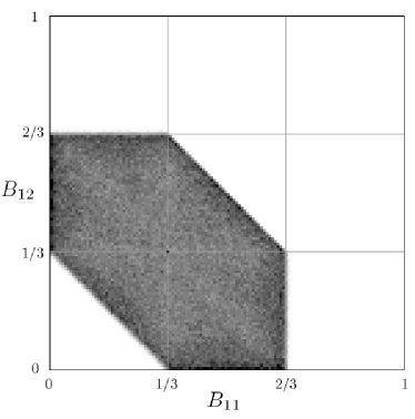
To visualize numerical results we selected the cases for which . Such a two dimensional cross-section of the Birkhoff polytope has a shape of a hexagon at the plane , centered at the center of the body, . Figure 3 shows the probability distribution along this section, obtained from these realizations of the algorithm which produce bistochastic matrices inside a layer of width along the section.
As expected for the critical value of the Dirichlet parameter, the resulting distribution is flat in the vicinity of the center of the polytope. However, this distribution is not globally uniform and shows a slight enhancement of the probability (darker color) along the boundary of the polytope.
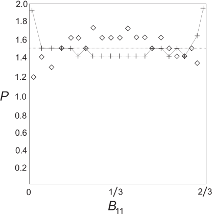
This feature is further visible in Fig 4 , which shows a comparison of the results obtained for two different initial measures on a one–dimensional cross section of Fig. 3 . Although the measure obtained for the critical parameter is indeed uniform in the vicinity of the center, namely around , the measure induced by random stochastic matrices with the flat measure, , displays similar properties. Since for larger matrix size the value of the optimal parameter tends to unity as , it seems reasonable to generate random bistochastic matrices of a larger size initiating the iterative Algorithm (1) with random stochastic matrices distributed according to the uniform measure, (i.e. each column is generated independently according to the Dirichlet distribution with ).
5 Estimation of the volume of the Birkhoff polytope
The set of bistochastic matrices of size forms a convex polytope in . Its volume with respect to the Euclidean measure is known for [5, 6]. The concrete numbers depend on the normalization chosen. For instance, in the simplest case the set forms an interval , any point of which corresponds to the bistochastic matrix, . If the range of the single, independent element is concerned, the relative volume of the polytope reads . On the other hand, if we regard this set as an interval in , its length is equal to the volume of the Birkhoff polytope, . In general, both definitions of the volumes are related by [12]
| (40) |
In Section 3 we derived formula (37) , giving the probability distribution at the center of the Birkhoff polytope induced by the Dirichlet measure on the space of input stochastic matrices. If all Dirichlet parameters are equal to for then formula (37) simplifies to
| (41) |
Making use of the Stirling expansion
| (42) |
and plugging it into eq. (41) we obtain an approximation valid for a large matrix size ,
| (43) |
For this distribution is flat in the vicinity of the center – compare eq. (39) . Assuming it is close to uniform in the entire Birkhoff polytope, we obtain an approximation of its relative volume, . Substituting into (43) we arrive at
| (44) |
Making use of the expansion we can express the value of by the Euler gamma constant The result is .
Interestingly, the above approximation is identical, up to a value of this constant, with the recent result of Canfield and Mackay [12]. Making use of the relation (40) we see that their asymptotic formula for the volume of the Birkhoff polytope is consistent with eq. (44) for . This fact provides a strong argument that the distribution generated by the Dirichlet measure with , is close (but not equal) to the uniform distribution inside the Birkhoff polytope. Furthermore, the initially flat distribution of the stochastic matrices, obtained for , leads to yet another reasonable approximation for the relative volume of , equivalent to (44) with .
6 Concluding Remarks
In this paper we introduced several ensembles of random stochastic matrices. Each of them can be considered as an ensemble of initial points used as input data for the Sinkhorn Algorithm, which generates bistochastic matrices. Thus any probability measure in the set of stochastic matrices induces a certain probability measure in the set of bistochastic matrices.
Let us emphasize that the iterative procedure of Sinkhorn [10] applied in this work, covers the entire set of bistochastic matrices. This is not the case for the ensemble of unistochastic matrices, which are obtained from a unitary matrix by squaring moduli of its elements. Due to unitarity of the matrix is bistochastic, and the Haar measure on induces a certain measure inside the Birkhoff polytope [20]. However, for , this measure does not cover the entire Birkhoff polytope since in this case there exist bistochastic matrices which are not unistochastic [1, 20].
In the general case of arbitrary we derive an integral expression representing the probability distribution inside the –dimensional Birkhoff polytope of bistochastic matrices. In the simplest case of it is straightforward to obtain explicit formulae for the probability distribution in the set of bistochastic matrices induced by the ensemble of stochastic matrices, in which both columns are independent. Furthermore, we find that to generate the uniform (flat) measure, , one needs to start with random stochastic matrices of size distributed according to eq. (31) , for which both columns are correlated.
For an arbitrary the integral form for the probability distribution can be explicitly worked out for a particular point — the flat, van der Waerden matrix (32) located at the center of the Birkhoff polytope. In this case we obtain an explicit formula for the probability distribution at this point as a function of the parameters defining the Dirichlet distribution for each column of the initially random stochastic matrix. Expanding the probability density in the vicinity of we find the condition for the optimal parameters , for which the density is flat in this region. Discrepancy of the measure constructed in this way from the uniform distribution is numerically analyzed in the case .
This measure is symmetric with respect to permutations of rows and columns of the matrix and for large it tends to the uniform measure in the set of bistochastic matrices. For large the optimal Dirichlet parameter tends to unity as . Thus we may suggest a simplified procedure of taking the initial stochastic matrices according to the flat measure, . Each column of such a random stochastic matrix is drawn independently and it consists of numbers distributed uniformly in the simplex . With an initial matrix constructed in this way we are going to run Algorithm (1). Such a procedure is shown to work fine already for . We tend to believe that this scheme of generating random bistochastic matrices could be useful for several applications in mathematics, statistics and physics.
Assuming that a given probability measure in a compact set is flat, the value of the probability density at an arbitrary point gives us an information about the Euclidean volume of this set, . We were pleased to find that the optimal algorithm for generating random bistochastic matrices is characterized by an inverse probability at the center of the polytope which displays the same dependence on the dimension as the volume of the Birkhoff polytope, Vol, derived in [12].
Although in this paper we analyzed dynamics in the classical probability simplex, the main idea of the algorithm may be generalized for the quantum dynamics. In such a case a stochastic matrix corresponds to a stochastic map (so called quantum operation), which sends the set of quantum states (Hermitean, positive matrices of trace one) into itself [8]. A quantum stochastic map is called bistochastic, if it preserves the maximally mixed state, . To generate random bistochastic maps one can use an analogous technique of alternating projection onto the subspaces in which a given map or its dual is stochastic. Such an algorithm suitable for the quantum problem, was proposed independently by Audenaert and Scheel [13]. First results concerning various measures induced into the set of quantum stochastic maps are presented in [25].
Acknowledgements
The authors gratefully acknowledges financial support provided by the EU Marie Curie Host Fellowships for Transfer of Knowledge Project COCOS (contract number MTKD–CT–2004–517186) and the SFB/Transregio–12 project financed by DFG and the Polish Ministry of Science under the grant number 1 P03B 042 26 .
Appendix A
In this appendix we demonstrate that the Algorithm (2) suitable for analytical calculations is equivalent with the Sinkhorn Algorithm (1).
To apply the former Algorithm (2) one takes some initial matrix and makes it bistochastic by means of left– and right–multiplication by two matrices , and . The latter are limits of convergent sequences of diagonal matrices and and the finally .
In a similar way, Algorithm (1) performs the same task of transforming the initially stochastic matrix into a bistochastic matrix by alternating rows– and columns–normalization (R and C, for short), which in turn is the same of left– , respectively right–multiplication by diagonal matrices. Once a matrix is given to renormalize the row means to divide each of its elements by the factor ,
| (45a) | ||||
| Analogously, to renormalize the column means to divide each of its elements by the factor , | ||||
| (45b) | ||||
Let us now run the Algorithm 1, taking as an input a generic , and set 1CRCRCR… to be the row–column renormalization sequence, where the first symbol 1 denotes the dummy operation
| (46a) | ||||
| Now we start with equations (45b) | ||||
| (46b) | ||||
| followed by (45a) | ||||
| (46c) | ||||
| The next two steps are | ||||
| (46d) | ||||
| and | ||||
| (46e) | ||||
so that the iteration procedure can be written as
| (47) |
The latter form can be rewritten more compactly,
| (48) |
where we introduced new variables
| (49) |
Equation (47) is formally equivalent to (7), the only difference being in the number of component of vectors, respectively , that are processed: in Algorithm (1) one iterates all , whereas in Algorithm (2) the element is fixed to unity in each step. We know that the solution of the limit equation for is not unique. But the only non-uniqueness is due to multiplication by a fixed factor .
Appendix B
In this appendix we present the basic steps allowing one to derive the central result of this work - the second order expansion (36) around the center of the Birkhoff polytope of the probability distribution generated by Dirichlet random stochastic matrices.
Since , it is convenient to expand . We denote the sum of the Dirichlet parameters for each column by and start with the following integral
| (50) |
Expanding the function ,
| (51) |
and then we get
| (52) |
Thus we have to integrate the following expression for an arbitrary vector of parameters
| (53) |
Here , so the integral reads
| (54) |
with
| (55) |
This expression, completely symmetric in all variables , … , allows us to calculate the expansion of the integral (52) :
| (56) |
Therefore we need
| (57) |
Thus the second term in (56) is
| (58) |
For the third term we have
| and using from (35) the relation we get | |||
| (59) | |||
| For the fourth term we obtain | |||
| (60) | |||
Finally, expression (56) yields:
| (61) |
In principle we are able to calculate all higher terms. There are two other terms to be expanded: and . For the latter we have
| (62) |
In the last line we made use of equation (35) and we introduced the circulant [24] matrix . As it can be verified by direct matrix multiplication, the inverse of reads . Hence, factorizing the determinant of the product in the product of determinants, it follows from (62)
| (63) | |||
| Observe that the index labels the columns of the matrix , whereas runs from to , since we are going to consider and not . Using the property of circulant matrices [24], we can determine the spectrum of , consisting of a simple eigenvalue and another one equal to , of multiplicity . Thus and eq. (35) and (63) yield | |||
| (64) | |||
From the identity , with the substitution we get
so that, choosing for the ’s contributions in equation (64) , we get and therefore
| (65) |
Finally we use the expansion
| (66) |
Now, substituting (61) and (65–66) into (34) , we obtain the final formula for the resulting probability distribution around the center of the Birkhoff polytope given by ((36)).
Appendix C
In this appendix we provide the third order expansion of the probability distribution at . The result obtained implies that it is not possible to find an ensemble of stochastic matrices characterised by the Dirichlet distribution, which induces a distribution flat up to the third order at the center of the Birkhoff polytope. Furthermore, we provide an estimation, that is how the asymmetry of the optimal distribution around changes with .
For general the output distribution behaves like at the center, with
| (67) |
From now on, symbols like
denote the
probability densities obtained from the input described by the string
consisting of
Dirichlet exponents equal.
Since , the distribution is Gaussian
for .
In order to study the deviations from the Gaussian distribution, we now study the third order contribution to of eq. (34) , in the case . Under the latter hypothesis, many terms of the kind vanish for (35) so such terms will be omitted.
The distribution (34) can be factorized into a product of three factors:
-
•
gives a contribution
(68) -
•
gives no order contribution (just the overall factor already present in (65)) ;
- •
Using the same reasoning as in Appendix B, including now the new contributions (68–69), we arrive at the order contribution for ,
| (70) |
The last term reads
| (71) |
It follows from (35) , that , so Multiplying this equality by and summing over one gets
| (72a) | ||||
| Similarly | ||||
| and using (72a) we arrive at | ||||
| (72b) | ||||
Substituting eqs. (72) into (71) one obtains
| Now we use (55) | ||||
| (73) | ||||
Thus, from (70) , the third order contribution to is
| (74) |
and, near the center , has the following structure:
| (75) |
Assuming that (so ) we may then find from (36) the value of the constant ,
| (76a) | ||||
| Similarly eq. (74) implies that the third constant reads, | ||||
| (76b) | ||||
Adjusting appropriately to the size of the matrix one may find such a value of the Dirichlet parameter that or are equal to zero. However, if we set to zero, the parameter is non zero, so the third order terms remain in eq. (75). Thus we have shown that it is not possible to find an initial Dirichlet distribution which gives the output distribution uniform in the vicinity of the center of the Birkhoff polytope up to the third order. A power expansion of gives
| (77) |
Thus the scale of the asymmetry is so it cannot be seen for that means if .
References
- [1] A. W. Marshall and I. Olkin, Inequalities: theory of majorization and its applications, Academic Press, New York, NY, 1979.
- [2] R. Bhatia, Matrix analysis, Springer–Verlag, New York, NY, 1997.
- [3] J. E. Cohen, Kemperman J. H. B. and G. Zbaganu, Comparisons of stochastic matrices, with applications in information theory, statistics, economics, and population sciences, Birkhäuser, Boston, MA, 1998.
- [4] R. A. Brualdi Combinatorial matrix classes, Encyclopedia of mathematics and its applications, Cambridge University Press, 2006.
- [5] Chan C.S. and Robbins D.P., On the volume of the polytope of doubly stochastic matrices, Exp. Math. 8(3), 291–300 (1999).
- [6] M. Beck and D. Pixton, The Ehrhart Polynomial of the Birkhoff Polytope, Discrete & Computational Geometry 30(4), 623–637 (2003).
- [7] J. A. De Loera, F. Liu and R. Yoshida, Formulas for the volumes of the polytope of doubly–stochastic matrices and its faces, arXiv:math/0701866v1 [math.CO], 2007.
- [8] I. Bengtsson and K. Życzkowski, Geometry of Quantum States: An Introduction to Quantum Entanglement, Cambridge University Press, Cambridge, 2006.
- [9] H. H. Bauschke and J.M. Borwein, SIAM Rev. 38, 367-426 (1996).
- [10] R. Sinkhorn, A relationship between arbitrary positive matrices and doubly stochastic matrices, Ann. Math. Stat. 35, 876-879 (1964).
- [11] R. Sinkhorn and P. Knopp, Concerning non-negative matrices and doubly stochastic matrices, Pacific J. Math. 21(2), 343-348 (1967).
- [12] E. R. Canfield and B. D. McKay, The asymptotic volume of the Birkhoff polytope, arXiv:0705.2422v1 [math.CO], 2007.
- [13] K. M. R. Audenaert and S. Scheel, On random unitary channels, N. J. Phys. 10, 023011 (2008).
- [14] D. Djoković, Note on nonnegative matrices, Proc. Amer. Math. Soc. 25, 82-90 (1970).
- [15] P. B. Slater, A priori probabilities of separable quantum states, J. Phys. A: Math. Gen. 32(28), 5261–5275 (1999).
- [16] R. R. Tucci, Entanglement of Formation and Conditional Information Transmission, preprint quant-ph/0010041 (2000).
- [17] K. Życzkowski and H.-J. Sommers, Induced measures in the space of mixed quantum states, J. Phys. A: Math. Gen. 34(35), 7111–7125 (2001).
- [18] L. Devroye, Non–Uniform Random Variate Generation, Springer–Verlag, New York, Berlin, Heidelberg, Tokyo, 1986.
- [19] Mathematica 5.2, Wolfram Research, Inc., 2005.
- [20] W. Słomczyński, K. Życzkowski, M. Kuś, and H.-J. Sommers, Random unistochastic matrices, J. Phys. A: Math. Gen. 36(12), 3425–3450 (2003).
- [21] S. Barnett, Matrices: methods and applications, Oxford applied mathematics and computing science series, Clarendon Press, Oxford, 1990.
- [22] A. Berman and R. J. Plemmons, Nonnegative matrices in the mathematical sciences, Classics in applied mathematics. v.9., Ann. of Phys., Philadelphia, 1979.
- [23] D. S. Bernstein, Matrix mathematics: theory, facts, and formulas with application to linear systems theory, Princeton University Press, Princeton, 2005.
- [24] J. Hofbauer and K. Sigmund, Evolutionary games and population dynamics, Cambridge University Press, Cambridge, 1998.
- [25] W. Bruzda, V. Cappellini, H.-J. Sommers and K. Życzkowski, Random quantum operations, Phys. Lett. A 373, 320-324 (2009).