On the nature of the fast moving star S2 in the Galactic Center

Abstract

We analyze the properties of the star S2 orbiting the supermassive black hole at the center of the Galaxy. A high quality SINFONI H and K band spectrum obtained from coadding 23.5 hours of observation between 2004 and 2007 reveals that S2 is an early B dwarf (B0–2.5V). Using model atmospheres, we constrain its stellar and wind properties. We show that S2 is a genuine massive star, and not the core of a stripped giant star as sometimes speculated to resolve the problem of star formation so close to the supermassive black hole. We give an upper limit on its mass loss rate, and show that it is He enriched, possibly because of the presence of a magnetic field.

1. Introduction

The central parsec of our Galaxy hosts a large population of young massive stars (Krabbe et al., 1995; Paumard et al., 2006). Their presence is puzzling since according to standard theories, star formation should not happen so close to the supermassive black hole SgrA*: the tidal forces are so large that any molecular cloud should be disrupted before being able to collapse (Morris, 1993). For most of the young stars, the solution seems to be star formation in dense accretion disks as witnessed by the two counter-rotating flat stellar structures around SgrA* (Levin & Beloborodov, 2003; Genzel et al., 2003; Paumard et al., 2006). However, this attractive solution does not explain the so-called “S stars”, the group of objects located within one arcsecond (=0.038 pc) of the black hole. Their orbits are randomly oriented (Eisenhauer et al., 2005) and thus do not fit the accretion disk scenario. Spectroscopically identified as B stars (Ghez et al., 2003; Eisenhauer et al., 2005), their true nature as massive stars has been challenged: they have been proposed to be the hot, luminous cores of evolved red giant and/or AGB stars the envelope of which has been stripped by tidal interactions with SgrA* (Alexander, 2005; Davies & King, 2005). In that case, the problem of their formation process vanishes since they might very well have formed away from the hostile environment of the black hole before having migrated towards the Galactic Center. Such a process is too slow to explain the presence of short lived massive stars close to SgrA*. Hence, these S stars constitute a “paradox of youth” (Ghez et al., 2003).

In this letter, we analyze the properties of the brightest S-star – S2 – and show that it is a genuine massive star.

2. Observational data and models

To constrain the physical parameters of S2, a high quality spectrum is needed. Since the observation of the S stars is time consuming, the S/N ratio obtained in one night is usually limited to 10 at maximum. To increase this ratio, we have co-added all the S2 spectra obtained with SINFONI (Eisenhauer et al., 2003) in adaptive optics mode (0.0125″$\times$0.025″) on the VLT since 2004. This corresponds to a total integration time of 23.5 hours in K band. Each spectrum was carefully extracted by selection of source and background pixels from which nebular contamination was removed. Note however that this is not such a critical problem for S2 which has a large radial velocity so that the position of the stellar absorption core is blueshifted beyond the nebular emission. We have determined the combined spectrum by a cross-correlation technique. First, the position of the Br$\gamma$ line was estimated by a simple Gaussian fit to the line. From the such obtained radial velocities a first combined spectrum was calulated. This spectrum was then used to cross-correlate all individual spectra against it. This yielded better estimates for the radial velocities, which in turn were used to get a more accurate combined spectrum. This procedure was iterated until the result did not change anymore. The resulting spectrum shown in Fig. 1 has a S/N ratio of a few tens in the K band and a resolution of $\sim 4000$. The H band spectrum is noisier due to shorter observation time and higher extinction.

The main K band lines (He i 2.112 $\mu m$ and Br$\gamma$) are clearly identified. But we also detect several weak He i lines at 2.149, 2.161 and 2.184 $\mu m$. Similarly, one He i and three H i lines are identified for the first time in the H band . We do not see any trace of He ii 2.189 $\mu m$. With the current S/N ratio, this line would be detected if it had a depth of about 1% of the continuum level.

For the quantitative analysis of this spectrum, we used the atmosphere code CMFGEN (Hillier & Miller, 1998). It allows the computation of non-LTE atmosphere models including winds and line blanketing and is appropriate for hot massive stars. A description of the code is given in Hillier & Miller (1998), and we refer to Martins et al. (2007) for a summary of the procedure used to build the models. To derive the parameters of interest, we have run models with: 19000 $<T_{\rm eff}<$ 30000 K, 3.0 $<\log g<$ 4.75, 0.1 $<$ He/H $<$ 2.0 and 10^-8 $<\dot{\rm M}<$ 10^-5.5 M_⊙ yr^-1. These models and synthetic spectra included, in addition to H and He, C, N, O, Si, S and Fe. We adopted the solar abundances of Grevesse & Sauval (1998).

Figure 1.— Spectrum of S2 after addition of all the SINFONI observations since 2004. The main lines are indicated.

3. The nature of S2: a genuine B star

3.1. Spectroscopic classification

The spectrum shown in Fig. 1 is typical of an early B star (see also Ghez et al., 2003). Inspection of the atlases of Wallace & Hinkle (1997) and Hanson et al. (2005) shows that for late O stars, He ii 2.189 $\mu m$ is expected. We do not detect this line in spite of the good enough S/N ratio. For stars with spectral types later than B3, the He i lines vanish. Since we detect several of them, we can safely argue that S2 has a spectral type between B0 and B2.5. Fig. 12 of Hanson et al. (2005) shows that in supergiants and giants, Br$\gamma$ is clearly separated from He i 2.161 $\mu m$, while for dwarfs Br$\gamma$ is broad enough to merge with the He i line. This latter morphology is similar to what we observe for S2 (see below for a quantitative comparison). Hence, in addition to being spectroscopically identified as an early B star, we can conclude from these qualitative arguments that S2 is also a dwarf and not a supergiant/giant.

3.2. A mass estimate

The key question we want to answer here is the exact nature of S2. Spectroscopically, S2 is unambiguously an early B dwarf. However, this does not necessarilly mean that S2 is a young, massive star. It could be the core of an older, evolved star which would have lost its envelope through tidal interaction with SgrA* but would still spectroscopically look like a B star. In that case, the star could have formed far away from SgrA* before being dragged to its proximity and experiencing an envelope stripping. There would be no paradox of youth.

Recently, Davies & King (2005) and Dray et al. (2006) modeled this stripping process as well as the subsequent evolution of the remaining core in the vicinity of SgrA*. They showed that, under certain condition on the IMF and the capture rate, the population of S stars could be explained by tidal stripping. The argument is however based on the number of stars predicted at the position of the S stars in the HR diagram. Expressed differently, the conclusion comes from the fact that the modeled stripped stars can reach the luminosities and effective temperatures of B stars. But strictly speaking, this does not exclude that the S stars are genuine massive stars, which would lie at the same position in the HR diagram.

For that, the only parameter which can unambiguously be used is the stellar mass. The most massive stars able to experience envelope stripping are AGB stars. According to stellar evolution, such objects are the evolved descendents of main sequence stars with M $<$ 8 M_⊙. The core of such objects is actually much less massive: Table 4 of Forestini & Charbonnel (1997) shows that their mass is lower than 1 M_⊙. In the scenario explored by Dray et al. (2006), only stars having lost at least 99% of their envelope could explain the S stars. Thus, their mass should be at most $\sim$ 1 M_⊙.

To estimate the mass of S2, we can rely on gravity and radius: $M=gR^{2}/G$ where $g$ is the gravity, $R$ the radius and $G$ the gravitational constant. Gravity can be derived from the shape of Br$\gamma$, while radius is straightforwardly obtained from the knowledge of effective temperature and luminosity. Below, we explain how we proceeded to constrain these parameters.

Table 1Physical properties derived from our quantitative analysis for different $T_{\mathrm{eff}}$ appropriate for B0–2.5V stars.

$T_{\mathrm{eff}}$ [K]	19000	22000	25000	27000	30000
$\log\frac{L}{L_{\odot}}$	4.30	4.45	4.60	4.65	4.80
$\log g$	3.80	4.00	4.00	4.00	4.25
$\log g_{min}$	3.55	3.72	3.77	3.89	3.86
R [R⊙]	13.1	11.6	10.7	9.7	9.4
Rmin [R⊙]	11.4	10.1	9.3	8.5	7.3
Mmin [M⊙]	16.8	19.5	18.6	20.5	14.1
He/H [#]	1.20	0.50	0.45	0.55	0.80
He/Hmin [#]	0.85	0.25	0.25	0.30	0.30
$\dot{M}$ [$10^{-7}$M⊙ yr-1]	$<$3	$<$3	$<$3	$<3$	$<$3

Effective temperature. $T_{\mathrm{eff}}$ is usually derived from the ratio of lines from two consecutive ionization states: He i / He ii lines for O stars and Si iii / Si iv for early B stars. Unfortunately, S2 does not show He ii and Si lines in the K band. Hence, we can only rely on semi-quantitative arguments to estimate $T_{\mathrm{eff}}$. We have shown above that S2 is a B0V to B2.5V star. According to the recent studies of Dufton et al. (2006) and Trundle et al. (2007), such stars have 19000 $<$ $T_{\mathrm{eff}}$ $<$ 30000 K. We have thus run models for $T_{\mathrm{eff}}$ = 19, 22, 25, 27 and 30 kK.

Luminosity. To estimate the star’s luminosity, for each $T_{\mathrm{eff}}$  we adjusted $\log\frac{L}{L_{\odot}}$ in our models to match the absolute K band magnitude of S2. This magnitude is defined as $MK=mK-A_{K}-DM$ with $mK=14.0$ the observed magnitude of S2 (Paumard et al., 2006), $A_{K}=2.25$ the K band extinction at the position of S2 (Sch$\ddot{\rm o}$del et al., 2007) and $DM=14.50$ the distance modulus for a distance to the Galactic Center of 7.94 kpc (Eisenhauer et al., 2003). The resulting absolute K magnitude of S2 is -2.75. The range of values we obtain for $\log\frac{L}{L_{\odot}}$ is 4.30–4.80. In practice, the uncertainty of $\pm$0.2 on $A_{K}$ and 0.5 kpc on the distance to the Galactic Center translate into an uncertainty of about 0.12 in $\log\frac{L}{L_{\odot}}$.

Radius. The radius of the star is simply derived from $L=4\pi\sigma_{B}R^{2}T_{eff}^{4}$ ($\sigma_{B}$ being the Boltzmann constant). The minimum radius allowed by our study (corresponding also to the minimum mass of the star – see below) is estimated for a luminosity reduced by the uncertainty (0.12 dex). The values of $R_{min}$ are given in Table 1.

Gravity. $\log g$ was constrained from the shape of Br$\gamma$. Repolust et al. (2005) showed that its wings (resp. absorption core) get broader (resp. weaker) when gravity increases. For large $\log g$, the blue wing merges with the He i 2.161$\mu m$ line as discussed previously. Fig. 2 shows how the line profile changes when $\log g$ increases from 3.0 to 4.5 for $T_{\mathrm{eff}}$ = 22000 K. The best models correspond to $\log g$ $\sim$ 4.0. A quantification of the goodness of the fit in the Br$\gamma$ region of the spectrum was performed by means of a $\chi^{2}$ analysis. To minimize contamination by HeI, we used only the range 2.164-2.179$\mu m$. Fig. 3 shows the result of this analysis and confirms that $\log g$ = 4.0 is preferred. From this curve, we also derive a 3 $\sigma$ lower limit to $\log g$ ($\log g_{min}$). Table 1 shows the results for other $T_{\mathrm{eff}}$. The values of $\log g$ we obtain are all typical of a dwarf star ($\log g$$\sim$ 4.0, Trundle et al., 2007), confirming our previous “spectroscopic” findings.

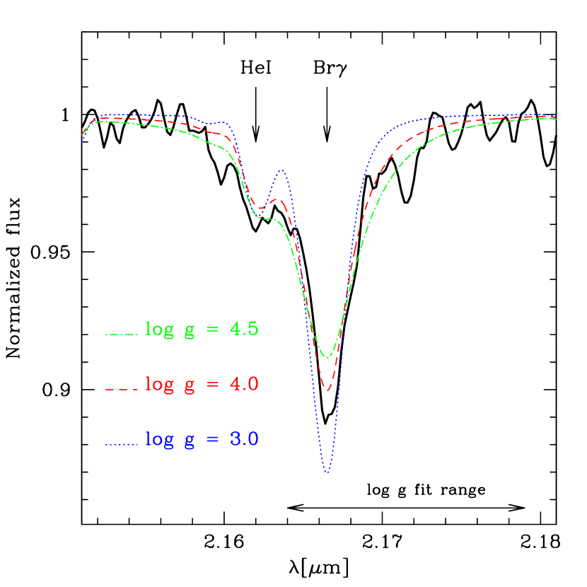
Figure 2.— Determination of $\log g$ for the case $T_{\mathrm{eff}}$ = 22000 K. The black solid line is the observed Br$\gamma$ line. The dashed (dotted, dot-dashed) line is a model with $\log g$ = 4.0 (3.00, 4.50). All other parameters are kept constant (especially He/H=0.5). The wavelength range used for the $\log g$ determination is indicated.

Figure 3.— $\chi^{2}$ as a function of $\log g$ for the $T_{\mathrm{eff}}$ = 22000 K model. The best fit model has $\log g$ = 4.0, as also seen from Fig. 2.

Rotational velocity. We derived a projected rotational velocity of 100$\pm$30 km s^-1. It best accounts for the shape of the He i 2.112 $\mu m$ doublet: for larger $V$ sin$i$ the lines merge into a single component, for lower values, they are too seperated. This value is commonly found for early B stars: according to Abt et al. (2002), $V$ sin$i$ = 127$\pm$8 (108$\pm$8) km s^-1 for B0–2V (B3–5V) stars.

Table 1 summarizes, for each $T_{\mathrm{eff}}$, the values of $\log g$ and radius. Since we want to test if S2 is the core of an AGB star, we also give the minimum mass of S2. All our estimates are larger than 14.1 M_⊙. This is larger than the initial mass of AGB stars, and consequently is well above the mass of the core of such a star. From that, one can thus safely conclude that S2 is not a stripped AGB star, and is really a genuine B star.

4. Mass loss rate and Helium content

4.1. Mass loss rate

Below a certain threshold, Br$\gamma$ is insensitive to $\dot{M}$. When $\dot{M}$ increases above this limit, the Br$\gamma$ absorption profile is progressively filled by emission. By determining this threshold, we can set an upper limit on the mass loss rate of S2 (see Fig. 4). In practice, the quantity we constrain is the wind density $\rho=\dot{M}/(4\pi R^{2}v_{\infty})$ (where $R$ is the stellar radius and $v_{\infty}$ the terminal velocity). Deriving a mass loss rates implies we know $v_{\infty}$. Since the lines we observe in the S2 K band spectrum are insensitive to $v_{\infty}$, we have to assume values. Terminal velocities of B dwarfs are difficult to estimate since the winds are usually weak and the spectra do not show P-Cygni lines or emission lines from which it is usually derived. Hence, we have adopted $v_{\infty}$ = 1000 km s^-1 which is appropriate for late O dwarfs (e.g. Bouret et al., 2003). If $v_{\infty}$ would be lower than 1000 km s^-1, estimated mass loss rates would be lower. Our assumptions thus lead to conservative upper limits of $\dot{M}$ $\lesssim 3\times 10^{-7}$ M_⊙ yr^-1. This is lower than $\dot{M}$ required by Loeb (2004) to feed SgrA* without transport of angular momentum.

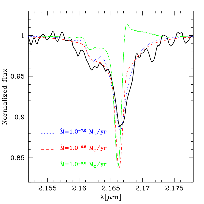
Figure 4.— Effect of mass loss on Br$\gamma$. When $\dot{M}$ increases, Br$\gamma$ starts to depart from a pure absorption to an emission profile. Characterizing the value of $\dot{M}$ for which this occurs provides an upper limit on the mass loss rate of S2.

4.2. Helium content

The near infrared spectrum of S2 is dominated by H and He lines. We thus could constrain the He/H abundance ratio. Qualitatively, when this ratio increases, all He i lines have stronger absorption profiles, while H i lines get weaker. In practice, we used the He i 2.149 $\mu m$ and He i 2.184 $\mu m$ lines to constrain He/H since these lines are almost insensitive to microturbulence, which is not the case of He i 2.112 $\mu m$ and He i 2.161 $\mu m$. Fig. 5 shows the changes in the He i line profiles when He/H is varied between 0.1 and 0.5 (model with $T_{\mathrm{eff}}$ = 22000 K). We find that the He/H ratio varies from about 0.45 at $T_{\mathrm{eff}}$ = 25000 K up to as high as 1.20 at $T_{\mathrm{eff}}$ = 19000 K. We proceeded as for $\log g$ ($\chi^{2}$ analysis) to derive a 3 $\sigma$ lower limit on the value of He/H. All these lower limits are larger than 0.25, confirming that S2 is He enriched.

With He/H $>$ 0.25, S2 falls into the category of the so-called “He rich” stars, a class of B stars with He/H between 0.3 and 10 (Smith, 1996). Interestingly, these peculiar stars have a very narrow distribution of spectral types centered around B2, similar to what we find for S2 (B0–2.5V). The best studied He-rich star is $\sigma$ OriE. The origin of its surface abundance pattern is explained by a combination of specific wind properties and magnetic field. The star should have a wind weak enough for ion decoupling to occur, i.e. the radiative acceleration, essentially due to metals, is not redistributed among the passive plasma (mainly H and He) because of a too low density and reduced Coulomb forces (Krti$\breve{\rm c}$ka & Kubát, 2001). In that case, Helium might accumulate at the surface of the star. But this extra Helium can remain on the surface only if turbulence, and its associated mixing effect, is suppressed. This calls for a magnetic field strong enough to freeze the stellar surface (Hunger & Groote, 1999). Our upper limit on the mass loss rate of S2 is consistent with a relatively weak wind. In this scenario, chemical inhomogeneities (spots) are expected on the surface as a result of the interplay between the magnetic field geometry and the wind. We cannot test this prediction with our observations since we do not spatially resolve the stellar surface of S2. Similarly, no CNO abnormalities are expected in this model, which we cannot test either due to the absence of CNO lines (observed and expected) in the near-IR spectrum of S2.

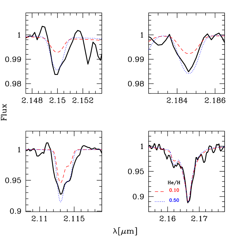
Figure 5.— Determination of He/H. The black solid line is the observed spectrum of S2. The red dashed (blue dotted) line is a model with He/H=0.10 (0.50). $T_{\mathrm{eff}}$ = 22000 K and $\log g$= 4.0. The He rich model is required to fit the S2 spectrum.

If the wind is strong enough to develop into a normal homogenous outflow, one might still observe a significant He enrichment if the star has a magnetic field and rotates fast enough. Indeed Maeder & Meynet (2005) predict that a strong (10⁴ G) magnetic field can lead to solid body rotation of the star. This favors the diffusion of species by meridional circulation. As a consequence, a star can experience strong surface He enrichment: Fig. 10 of Maeder & Meynet (2005) shows that a 15 M_⊙ star can reach a He mass fraction of 0.3 (around 0.12 in He/H) in 12 Myr. Contrary to the previous scenario, large N and reduced C abundances are also expected.

In view of the available models and of the currently known stellar properties, we thus tentatively propose that S2 is a magnetic star.

References

- Abt et al. (2002) Abt, H., et al., 2002, ApJ, 573, 389
- Alexander (2005) Alexander, T, 2005, PhR, 419, 65
- Bouret et al. (2003) Bouret, J. C., et al., 2003, ApJ, 595, 1182
- Davies & King (2005) Davies, M.B. & King, A.R., 2005, ApJ, 624L, 25
- Dray et al. (2006) Dray, L.M., et al., 2006, MNRAS, 372, 31
- Dufton et al. (2006) Dufton, P.L., et al., 2006, A&A, 457, 265
- Eisenhauer et al. (2003) Eisenhauer, F., et al., 2003, ApJ, 597L, 121
- Eisenhauer et al. (2003) Eisenhauer, F., et al., 2003, SPIE, 4841, 1548
- Eisenhauer et al. (2005) Eisenhauer, F., et al., 2005, ApJ, 628, 246
- Figer et al. (1999) Figer, D.F., et al., 1999. ApJ, 506, 384
- Forestini & Charbonnel (1997) Forestini, M. & Charbonnel, C., 1997, A&AS, 123, 241
- Genzel et al. (2003) Genzel, R., et al., 2003, ApJ, 594, 812
- Ghez et al. (2003) Ghez, A.M., et al., 2003, ApJ, 586L, 127
- Grevesse & Sauval (1998) Grevesse, N. & Sauval, A.J., 1998, SSRv, 85, 161
- Hanson et al. (2005) Hanson, M.M., et al., 2005, ApJS, 161, 154
- Hillier & Miller (1998) Hillier, D.J., Miller, 1998, ApJ, 496, 407
- Hunger & Groote (1999) Hunger, K. & Groote, D., 1999, A&A, 351, 554
- Krabbe et al. (1995) Krabbe, A., et al., 1995, ApJ, 447L, 95
- Krtika & Kubát (2001) Krtika, J. & Kubát, J., 2001, A&A, 369, 222
- Levin & Beloborodov (2003) Levin, Y. & Beloborodov, A.M. , 2003, ApJ, 590L, 33
- Loeb (2004) Loeb, A., 2004, MNRAS, 350, 725
- Martins et al. (2007) Martins, F. et al., 2007, A&A, 468, 233
- Maeder & Meynet (2005) Meynet, G., Maeder, A., 2005, A&A, 440, 1041
- Morris (1993) Morris, M., 1993, ApJ, 408, 496
- Paumard et al. (2006) Paumard, T., et al., 2006, ApJ, 643, 1011
- Repolust et al. (2004) Repolust, T. et al., 2004, A&A, 415, 349
- Repolust et al. (2005) Repolust, T. et al., 2005, A&A, 440, 261
- Schdel et al. (2007) Schdel, R., et al., 2007, A&A, 469, 125
- Smith (1996) Smith, K.C., 1996, Ap&SS, 237, 77
- Trundle et al. (2007) Trundle, C., et al., 2007, A&A, 471, 625
- Wallace & Hinkle (1997) Wallace, L., Hinkle, K., 1997, ApJS, 111, 445