Structural parameters of star clusters: relations among light, mass and star-count radial profiles and the dependence on photometric depth

Abstract

Context. Structural parameters of model star clusters are measured in radial profiles built from number-density, mass-density and surface-brightness distributions, assuming as well different photometric conditions.

Aims. Determine how the core, half-star count and tidal radii, as well as the concentration parameter, all of which are derived from number-density profiles, relate to the equivalent radii measured in near-infrared surface-brightness and mass-density profiles. We also quantify changes in the resulting structural parameters due to depth-limited photometry.

Methods. Star clusters of different ages, structure and mass functions are modelled by assuming that the radial distribution of stars follows a pre-defined analytical form. Near-infrared surface brightness and mass-density profiles result from mass-luminosity relations taken from a set of isochrones. Core, tidal and half-light, half-mass and half-star count radii, together with the concentration parameter, are measured in the three types of profiles, which are built under different photometric depths.

Results. While surface-brightness profiles are almost insensitive to photometric depth, radii measured in number-density and mass-density profiles change significantly with it. Compared to radii derived with deep photometry, shallow profiles result in lower values. This effect increases for younger ages. Radial profiles of clusters with a spatially-uniform mass function produce radii that do not depend on depth. With deep photometry, number-density profiles yield radii systematically larger than those derived from surface-brightness ones.

Conclusions. In general, low-noise surface-brightness profiles result in uniform structural parameters that are essentially independent of photometric depth. For less-populous star clusters, those projected against dense fields and/or distant ones, which result in noisy surface-brightness profiles, this work provides a quantitative way to estimate the intrinsic radii by means of number-density profiles built with depth-limited photometry.

1 Introduction

Star clusters are a powerful tool in the investigation of Galaxy structure and dynamics, star formation and evolution processes, and as observational constraints to N-body codes. This applies especially to the long-lived and populous globular clusters (GCs) that, because of their relatively compact nature, can be observed in most regions of the Galaxy, from near the center to the remote halo outskirts.

In general terms, the structure of most star clusters can be described by a rather dense core and a sparse halo, but with a broad range in the concentration level. In this context, the standard picture of a GC assumes a isothermal central region and a tidally truncated outer region (e.g. Binney & Merrifield 1998). Old GCs, in particular, can be virtually considered as dynamically relaxed systems (e.g. Noyola & Gebhardt 2006). During their lives clusters are continually affected by internal processes such as mass loss by stellar evolution, mass segregation and low-mass star evaporation, and external ones such as tidal stress and dynamical friction e.g. from the Galactic bulge, disk and giant molecular clouds (e.g. Khalisi et al. 2007; Lamers et al. 2005; Gnedin & Ostriker 1997). Over a Hubble time, these processes tend to decrease cluster mass, which may accelerate the core collapse phase for some clusters (Djorgovski & Meylan 1994, and references therein). Consequently, these processes, combined with the presence of a central black hole (in some cases) and physical conditions associated to the initial collapse, can affect the spatial distribution of light (or mass) both in the central region and at large radii (e.g. Gnedin et al. 1999; Noyola & Gebhardt 2006).

It is clear from the above that crucial information related to the early stages of Galaxy formation, and to the cluster dynamical evolution, may be imprinted in the present-day internal structure and large-scale spatial distribution of GCs (e.g. Mackey & van den Bergh 2005; Bica et al. 2006). To some extent, this reasoning can be extended to the open clusters (OCs), especially the young, which are important to determine the spiral arm and disk structures and the rotation curve of the Galaxy (e.g. Friel 1995; Bonatto et al. 2006). Consequently, the derivation of reliable structural parameters of star clusters, GCs in particular, is fundamental to better define their parameter space. This, in turn, may result in a deeper understanding of the formation and evolution processes of the star clusters themselves and the Galaxy.

Three different approaches have been used to derive structural parameters of star clusters. The more traditional one is based on the surface-brightness profile (SBP), which considers the spatial distribution of the brightness of the component stars, usually measured in circular rings around the cluster center. The compilation of Harris (1996, and the 2003 update) presents a basically uniform set of parameters for 150 Galactic GCs. Among their structural parameters, the core ($\rm R_{c}$), half-light ($\rm R_{hL}$) and tidal ($\rm R_{t}$) radii, as well as the concentration parameter $c=\log(\mbox{$\rm R_{t}$}/\mbox{$\rm R_{c}$})$, were based mostly on the SBP database of Trager et al. (1995). SBPs do not necessarily require cluster distances to be known, since the physically relevant information contained in them is essentially related to the relative brightness of the member stars. In principle, it is easy to measure integrated light. However, SBPs are more efficient near the cluster center than in the outer parts, where noise and background starlight may be a major contributor. Another potential source of noise is the random presence of bright stars, either from the field or cluster members, especially outside the central region in the less-populous GCs or most of the OCs. Structural parameters derived from such SBPs would certainly be affected. One way to minimise this effect is the use of wide rings throughout the whole radius range, but this would cause spatial resolution degradation on the profiles, especially near the center.

The obvious alternative to SBPs is to use star counts to build radial density profiles (RDPs), in which only the projected number-density of stars is taken into account, regardless of the individual star brightness. This technique is particularly appropriate for the outer parts, provided a statistically significant, and reasonably uniform, comparison field is available to tackle the background contamination. On the other hand, contrary to SBPs, RDPs are less efficient in central regions of populous clusters where the density of stars (crowding) may become exceedingly large. In such cases it may not be possible to resolve individual stars with the available technology.

Finally, a more physically significant profile can be built by mapping the cluster’s stellar mass distribution, which essentially determines the gravitational potential and drives most of the dynamical evolution. However, mass density profiles (MDPs) not only are affected by the same technical problems as the RDPs but, in addition, the cluster distance, age and a reliable mass-luminosity relation are necessary to build them.

In principle, the three kinds of profiles are expected to yield different values for the structural parameters under similar photometric conditions, since each profile is sensitive to different cluster parameters, especially the age and dynamical state. Qualitatively, the following effects, basically related to dynamical state, can be expected. Large-scale mass segregation drives preferentially low-mass stars towards large radii (while evaporation pushes part of these stars beyond the tidal radius, into the field), and high-mass stars towards the central parts of clusters. If the stellar mass distribution of an evolved cluster can be described by a spatially variable mass function (MF) flatter at the cluster center than in the halo, the resulting RDP (and MDP) radii should be larger than SBP ones. The differences should be more significant for the core than the half and tidal radii, since the core would contain, on average, stars more massive than the halo and especially near the tidal radius. Besides, the presence of bright stars preferentially in the central parts of young clusters (Bonatto & Bica 2005 and references therein) should as well lead to smaller SBP core and half-light radii than the respective RDP ones.

Another relevant issue is related to depth-limited photometry. When applied to the observation of objects at different distances, depth-limited photometry samples stars with different brightness (or mass), especially at the faint (or low-mass) end. Thus, it would be interesting to quantify the changes produced in the derived parameters when RDPs, MDPS and SBPs are built with depth-limited photometry, as well as to check how the structural parameters derived from one type of profile relate to the equivalent radii measured in the other profiles.

In the present work we face the above issues by deriving structural parameters of star clusters built under controlled conditions, in which the radial distribution of stars follows a pre-established analytical profile, and field stars are absent. Effects introduced by mass segregation (simulated by a spatially variable mass function), age and structure are also considered. This work focuses on profiles built in the near-infrared range. The main goal of the present work is to examine relations among structural parameters measured in the different radial profiles, built under ideal conditions, especially noise-free photometry and as small as possible statistical uncertainties (using a large number of stars). In this sense, the results should be taken as upper-limits.

Table 1: Model star cluster specifications

Model	$R_{t}/R_{c}$	c	$\chi_{0}$	$\chi_{t}$	Age	$\rm[Fe/H]$	$m_{i}$	$m_{s}$	$\langle m\rangle$	$\rm M_{J}(TO)$	$\rm M_{J}(bright)$	$\rm M_{J}(faint)$
					(Myr)		($\rm M_{\odot}$)	($\rm M_{\odot}$)	($\rm M_{\odot}$)	(mag)	(mag)	(mag)
(1)	(2)	(3)	(4)	(5)	(6)	(7)	(8)	(9)	(10)	(11)	(12)	(13)
GC-A	5	0.7	0.00	1.35	$10^{4}$	$-1.5$	0.15	1.02	0.43	$+2.86$	$-2.14$	$+9.12$
GC-B	20	1.3	0.00	1.35	$10^{4}$	$-1.5$	0.15	1.02	0.43	$+2.86$	$-2.14$	$+9.12$
GC-C	20	1.3	0.00	0.00	$10^{4}$	$-1.5$	0.15	1.02	0.46	$+2.86$	$-2.14$	$+9.12$
GC-D	40	1.6	0.00	1.35	$10^{4}$	$-1.5$	0.15	1.02	0.43	$+2.86$	$-2.14$	$+9.12$
OC-A	15	1.2	0.30	1.35	$10^{3}$	$\leavevmode\nobreak\ \leavevmode\nobreak\ 0.0$	0.15	2.31	0.59	$+0.32$	$-2.68$	$+9.18$
OC-B	15	1.2	0.30	1.35	$100$	$\leavevmode\nobreak\ \leavevmode\nobreak\ 0.0$	0.15	5.42	0.92	$-1.82$	$-4.82$	$+9.18$
OC-C	15	1.2	0.30	1.35	$10$	$\leavevmode\nobreak\ \leavevmode\nobreak\ 0.0$	0.15	18.72	1.76	$-4.82$	$-8.82$	$+9.18$

• Col. 3: concentration parameter $c=\log(\mbox{$\rm R_{t}$}/\mbox{$\rm R_{c}$})$. Cols. 4 and 5: mass function slopes at the cluster center and tidal radius. Cols. 8-10: lower, upper and average star mass. Col. 11: absolute J magnitude at the turnoff (TO). Cols. 12 and 13: absolute J magnitude at the bright and faint ends.

Figure 1: Model star cluster specifications. Panel (a): a random selection of $n$ in the range $0\leq n\leq 1$ produces King-like RDPs in the range $0\leq R\leq\mbox{$\rm R_{t}$}$ (see Eq. 2). Panel (b): Radially-variable mass function slopes $\left(\frac{dN}{dm}\propto m^{-(1+\chi)}\right)$ used in the models. Panel (c): Padova isochrones used to simulate the mass-luminosity relation of the star cluster models. The 10 Gyr, $\mbox{$\rm[Fe/H]$}=-1.5$ metallicity isochrone is adopted in the globular cluster models. Panel (d): distribution of concentration parameters of the GCs in H03 with peaks at $c\approx 1.6,\leavevmode\nobreak\ 1.3,\leavevmode\nobreak\ {\rm and}\leavevmode\nobreak\ 0.7$. Panel (e): model fraction of stars brighter than $M_{J}=M_{J_{TO}}+\Delta_{TO}$. In all cases, the fraction of stars brighter than the TO ($M_{J_{TO}}$) is below the $1\%$ level.

This work is structured as follows. In Sect. 2 we present the star cluster models and build radial profiles with depth-limited photometry. In Sect. 3 we derive structural parameters from each profile, discuss their dependence on depth, and compare similar radii derived from the different types of profiles. In Sect. 4 we compare relations derived from model parameters with those of the nearby GC NGC 6397. Concluding remarks are given in Sect. 5.

2 The model star clusters

For practical reasons, the model star clusters are simulated by first establishing the number-density radial distribution. The approach we follow is to build star clusters of different ages and concentration parameters, with the spatial distribution of stars truncated at the tidal radius ($\rm R_{t}$). Stars are distributed with distances to the cluster center in the range $0\leq R\leq\mbox{$\rm R_{t}$}$, with the $R$ coordinate having a number-frequency given by a function similar to a King (1962) three-parameter surface-brightness profile. The mass and brightness of each star are subsequently computed according to a pre-defined mass function and mass-luminosity relation consistent with the model age. The last step is required for the derivation of the MDP and SBPs.

We point out that different, more sophisticated analytical models have also been used to fit the SBPs of Galactic and extra-Galactic GCs, other than King (1962) profile. The most commonly used are the single-mass, modified isothermal sphere of King (1966) that is the basis of the Galactic GC parameters given by Trager et al. (1995) and H03, the modified isothermal sphere of Wilson (1975), that assumes a pre-defined stellar distribution function (which results in more extended envelopes than King 1966), and the power-law with a core of Elson et al. (1987) that has been fit to massive young clusters especially in the Magellanic Clouds (e.g. Mackey & Gilmore 2003a,b,c). Each function is characterised by different parameters that are somehow related to the cluster structure. However, the purpose here is not to establish a “best” fitting function of the structure of star clusters in general. Instead, we want to quantify changes in the structural parameters, derived from RDPs, MDPs and SBPs of star clusters with the stellar distribution assumed to follow an analytical function, under different photometric conditions. We expect that changes in a given parameter should have a small dependence, if any at all, on the adopted functional form.

The adopted King-like radial distribution function is expressed as

$$\frac{dN}{2\pi\,R\,dR}=\sigma_{0}\left[\frac{1}{\sqrt{1+(R/R_{c})^{2}}}-\frac{1}{\sqrt{1+(R_{t}/R_{c})^{2}}}\right]^{2},$$ (1)

where $\sigma_{0}$ is the projected number-density of stars at the cluster center, and $\rm R_{c}$ and $\rm R_{t}$ are the core and tidal radii, respectively. Since structural differences are basically controlled by the ratio $\mbox{$\rm R_{t}$}/\mbox{$\rm R_{c}$}$, we set $\mbox{$\rm R_{c}$}=1$ in all models. Such a King-like RDP (for $\sigma_{0}=1.0$) is obtained by numerically inverting the relation (see App. A)

$$n(R)=\frac{x^{2}-4u(\sqrt{1+x^{2}}-1)+u^{2}\ln(1+x^{2})}{u^{2}\ln{u^{2}}-(u-1)(3u-1)},$$ (2)

where $x\equiv R/R_{c}$ and $u^{2}\equiv 1+(R_{t}/R_{c})^{2}$. Thus, a random selection of numbers in the range $0\leq n\leq 1$ produces a King-like radial distribution of stars with the radial coordinate in the range $0\leq R/R_{t}\leq 1$. The $R/R_{t}$ curves as a function of $n$ for the models considered in this work are shown in Fig. 1 (Panel a).

Once a given star has been assigned a radial coordinate, its mass is computed with a probability proportional to the mass function

$$\frac{dN}{dm}\propto m^{-(1+\chi)},$$ (3)

where the slope varies with $R$ according to $\chi=\chi(R)=\chi_{t}+(\chi_{t}-\chi_{0})(R/R_{t}-1)$, where $\chi_{0}$ and $\chi_{t}$ are the mass function slopes at the cluster center and tidal radius, respectively (Table 1 and Fig. 1). Thus, the presence of large-scale mass segregation in a star cluster can be characterised by a slope $\chi_{0}$ flatter than $\chi_{t}$. Mass values distributed according to Eq. 3 are obtained by randomly selecting numbers in the range $0\leq n\leq 1$ and using them in the relation of mass with $n\leavevmode\nobreak\ \rm{and\leavevmode\nobreak\ }\chi$ (App. A)

$$m=\left\{\begin{array}[]{lc}m_{i}\,(m_{s}/m_{i})^{n},&\rm{for\leavevmode\nobreak\ \chi=0.0,}\\ m_{s}/[(1-n)(m_{s}/m_{i})^{\chi}+n]^{1/\chi},&\rm{otherwise},\end{array}\right.$$ (4)

where $m_{i}$ and $m_{s}$ are the lower and upper mass values considered in the models (Table 1).

In what follows we adopt the 2MASS photometric system to build SBPs. Finally, the 2MASS $\rm J$, $\rm H$ and $\rm K_{s}$ magnitudes for each star are obtained according to the mass-luminosity relation taken from the corresponding model (Table 1) Padova isochrone (Girardi et al. 2002). For illustrative purposes the model isochrones are displayed in Fig. 1 (panel c).

The set of models considered here is intended to be objectively representative of the star cluster parameter space. For globular clusters we use the standard age of 10 Gyr and the spatially uniform metallicity $\mbox{$\rm[Fe/H]$}=-1.5$, which is typical of the metal-poor Galactic GCs (e.g. Bica et al. 2006). However, we note that abundance variations have been suggested to occur within GCs (e.g. Gratton et al. 2004). Basically, small to moderate metallicity gradients would produce slight changes in the colour and magnitude of the stars in different parts of the cluster, which has no effect on the (star-count derived) RDPs and MDPs. The effect on the SBPs may be small as well, provided that the magnitude bin used to build the SBPs is wide enough to accommodate such magnitude changes. As for the core/tidal structure we consider the ratios $R_{t}/R_{c}=40,\leavevmode\nobreak\ 20,\leavevmode\nobreak\ 15,\leavevmode\nobreak\ {\rm and}\leavevmode\nobreak\ 5$, or equivalently the concentration parameters $c=\log{(R_{t}/R_{c})\approx 1.6,\leavevmode\nobreak\ 1.3,\leavevmode\nobreak\ 1.2,\leavevmode\nobreak\ {\rm and}\leavevmode\nobreak\ 0.7}$, which roughly correspond to the peaks in the distribution of $c$ values presented by the regular (non-post core collapse) GCs given in H03 (Fig. 1, panel d). Models GC-A, B and D take into account mass segregation by means of a flat ($\chi_{0}=0.00$) mass function at the center and a Salpeter (1955) IMF ($\chi_{t}=1.35$) at the tidal radius. GC-C model is similar to GC-B, except that it considers a uniform, heavily depleted MF ($\chi_{0}=0.00$) throughout the cluster. OCs are represented by solar-metallicity models with the ages 10 Myr (to allow for the presence of bright stars in young OCs), 100 Myr (somewhat evolved OCs) and 1 Gyr (intermediate-age OCs), $R_{t}/R_{c}=15$ ($c\approx 1.2$) and a spatially variable MF (Table 1). The values of $c$ and the core/halo MF slopes are representative of OCs (Bonatto & Bica 2005). Another effect not considered here is differential absorption. In principle, low to moderate differential absorption should have a minimum effect on the radial profiles, because of the same reasons as those given above for the metallicity gradient. High values, on the other hand, would affect RDPs as well, because of a radially-dependent loss of stars due to depth-limited photometry. However, inclusion of this effect is beyond the scope of the present work.

As expected, the fraction of stars brighter than the turnoff (TO) in the resulting star cluster models is significantly smaller than 1% (Fig. 1, panel e). Thus, we had to use a total number of stars of $1\times 10^{9}$ in all models, so that the radial profiles resulted statistically significant (small $1\sigma$ Poisson error bars) especially at the shallowest magnitude depth.

2.1 Depth-varying radial profiles

The radial profiles were built considering all stars brighter than a given magnitude threshold, with the TO as reference. At the bright end, statistically significant GC profiles were obtained for $\mbox{$\rm\Delta_{TO}$}\equiv M_{J,th}-M_{J,TO}=-5$, where $M_{J,th}$ and $M_{J,TO}$ are the threshold and TO absolute magnitudes in the 2MASS $\rm J$ band. At the faint end, GC-models have $\mbox{$\rm\Delta_{TO}$}=6.3$. OC models have $\mbox{$\rm\Delta_{TO}$}=-3\leavevmode\nobreak\ {\rm and\leavevmode\nobreak\ }-4$ at the bright end, and $\mbox{$\rm\Delta_{TO}$}=8.9,\leavevmode\nobreak\ 11.0,\leavevmode\nobreak\ {\rm and}\leavevmode\nobreak\ 14.0$, at the faint end.

Starting at the bright magnitude end, RDPs, MDPs and SBPs were built considering stars with the $\rm J$ magnitude brighter than a given faint threshold, with the magnitude depth increasing in steps of $\mbox{$\rm\Delta_{TO}$}=1$, up to the respective faint magnitude end.

Figure 2 displays a selection of profiles corresponding to both extremes in magnitude depths, for the GC-D and OC-C models. These profiles are representative of the whole set of models, especially in terms of the small uncertainties associated with each radial coordinate. Reflecting the large differences in the number of stars at different photometric depths, the central values of the number and mass densities, and surface-brightness, vary significantly from the shallowest to the deepest profiles.

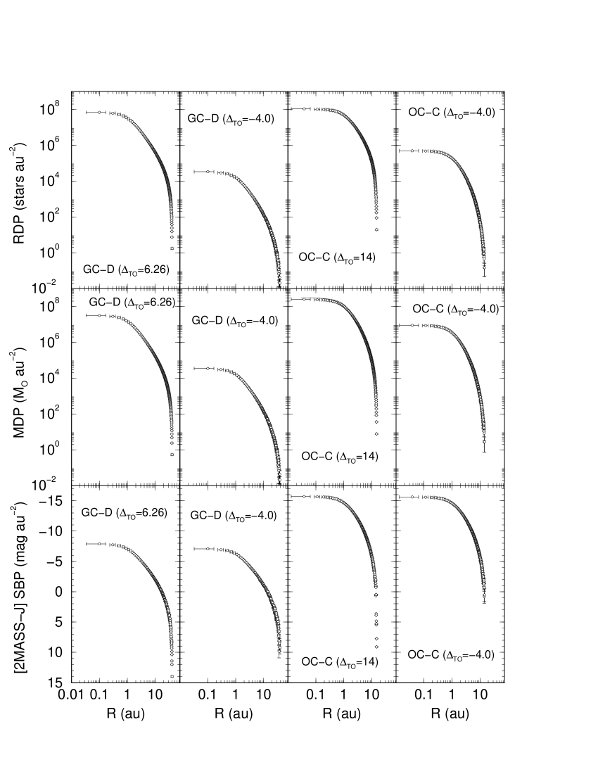
Figure 2: A selection of RDPs (top panels), MDPs (middle) and 2MASS $\rm J$ magnitude SBPs (bottom) that illustrate structural changes under different magnitude depths. Arbitrary units (au) are used both for the radial coordinate and projected area.

Table 2: Model star cluster structural parameters for different photometric depths

	RDP			MDP			SBP ($\rm J$ band)
$\Delta_{TO}$	$\rm R_{c}$	$\rm R_{hSC}$	$\rm R_{t}$	$\rm R_{c}$	$\rm R_{hM}$	$\rm R_{t}$	$\rm R_{c}$	$\rm R_{hL}$	$\rm R_{t}$
(mag)	(au)	(au)	(au)	(au)	(au)	(au)	(au)	(au)	(au)
(1)	(2)	(3)	(4)	(5)	(6)	(7)	(8)	(9)	(10)
	Model: GC-A; Input RDP parameters: $\mbox{$\rm R_{c}$}=1.0$, $\mbox{$\rm R_{t}$}=5.0$
$-5.0$	$0.78\pm({\dagger})$	$1.02\pm({\dagger})$	$4.61\pm 0.01$	$0.78\pm({\dagger})$	$1.02\pm({\dagger})$	$4.61\pm 0.01$	$0.75\pm 0.01$	$1.01\pm({\dagger})$	$4.80\pm 0.01$
$\leavevmode\nobreak\ 0.0$	$0.76\pm({\dagger})$	$1.02\pm({\dagger})$	$4.77\pm 0.01$	$0.76\pm({\dagger})$	$1.02\pm({\dagger})$	$4.77\pm 0.01$	$0.75\pm 0.01$	$1.01\pm({\dagger})$	$4.79\pm 0.01$
$+6.3$	$1.00\pm({\dagger})$	$1.19\pm({\dagger})$	$5.00\pm 0.01$	$0.92\pm({\dagger})$	$1.14\pm({\dagger})$	$4.91\pm({\dagger})$	$0.75\pm 0.01$	$1.03\pm({\dagger})$	$4.80\pm 0.01$
	Model: GC-B; Input RDP parameters: $\mbox{$\rm R_{c}$}=1.0$, $\mbox{$\rm R_{t}$}=20.0$
$-5.0$	$0.87\pm 0.01$	$2.03\pm({\dagger})$	$17.31\pm 0.08$	$0.87\pm 0.01$	$2.03\pm({\dagger})$	$17.31\pm 0.08$	$0.86\pm 0.01$	$2.04\pm 0.01$	$17.82\pm 0.05$
$\leavevmode\nobreak\ 0.0$	$0.83\pm 0.01$	$2.03\pm({\dagger})$	$18.72\pm 0.08$	$0.83\pm 0.01$	$2.03\pm({\dagger})$	$18.72\pm 0.08$	$0.86\pm 0.01$	$2.03\pm({\dagger})$	$17.80\pm 0.03$
$+6.3$	$1.00\pm({\dagger})$	$2.39\pm({\dagger})$	$20.00\pm({\dagger})$	$0.95\pm({\dagger})$	$2.27\pm({\dagger})$	$19.28\pm 0.03$	$0.86\pm 0.01$	$2.05\pm({\dagger})$	$17.80\pm 0.02$
	Model: GC-C; Input RDP parameters: $\mbox{$\rm R_{c}$}=1.0$, $\mbox{$\rm R_{t}$}=20.0$
$-5.0$	$1.00\pm({\dagger})$	$2.38\pm 0.01$	$20.02\pm 0.03$	$1.00\pm({\dagger})$	$2.38\pm 0.01$	$20.02\pm 0.04$	$1.00\pm({\dagger})$	$2.38\pm 0.01$	$19.94\pm 0.06$
$\leavevmode\nobreak\ 0.0$	$1.00\pm({\dagger})$	$2.39\pm({\dagger})$	$20.00\pm 0.01$	$1.00\pm({\dagger})$	$2.39\pm({\dagger})$	$20.00\pm 0.01$	$1.00\pm({\dagger})$	$2.39\pm({\dagger})$	$19.95\pm 0.03$
$+6.3$	$1.00\pm({\dagger})$	$2.39\pm({\dagger})$	$20.00\pm({\dagger})$	$1.00\pm({\dagger})$	$2.39\pm({\dagger})$	$20.00\pm({\dagger})$	$1.00\pm({\dagger})$	$2.39\pm({\dagger})$	$19.97\pm 0.03$
	Model: GC-D; Input RDP parameters: $\mbox{$\rm R_{c}$}=1.0$, $\mbox{$\rm R_{t}$}=40.0$
$-5.0$	$0.90\pm 0.01$	$2.81\pm 0.02$	$33.96\pm 0.19$	$0.90\pm 0.01$	$2.81\pm 0.02$	$33.96\pm 0.19$	$0.91\pm 0.01$	$2.82\pm({\dagger})$	$34.18\pm 0.05$
$\leavevmode\nobreak\ 0.0$	$0.86\pm 0.01$	$2.82\pm({\dagger})$	$37.15\pm 0.17$	$0.86\pm 0.01$	$2.82\pm({\dagger})$	$37.15\pm 0.17$	$0.91\pm 0.01$	$2.82\pm({\dagger})$	$34.00\pm 0.05$
$+6.3$	$1.00\pm({\dagger})$	$3.30\pm({\dagger})$	$39.99\pm 0.01$	$0.96\pm({\dagger})$	$3.14\pm({\dagger})$	$38.51\pm 0.07$	$0.91\pm 0.01$	$2.82\pm({\dagger})$	$34.20\pm 0.04$
	Model: OC-A; Input RDP parameters: $\mbox{$\rm R_{c}$}=1.0$, $\mbox{$\rm R_{t}$}=15.0$
$-3.0$	$0.82\pm 0.01$	$1.70\pm({\dagger})$	$12.85\pm 0.07$	$0.82\pm 0.01$	$1.70\pm({\dagger})$	$12.85\pm 0.07$	$0.81\pm 0.01$	$1.72\pm({\dagger})$	$13.18\pm 0.02$
$\leavevmode\nobreak\ 0.0$	$0.78\pm 0.01$	$1.72\pm({\dagger})$	$13.78\pm 0.06$	$0.78\pm 0.01$	$1.72\pm({\dagger})$	$13.78\pm 0.06$	$0.82\pm 0.01$	$1.72\pm({\dagger})$	$13.19\pm 0.02$
$+8.9$	$1.00\pm({\dagger})$	$2.08\pm({\dagger})$	$15.00\pm 0.01$	$0.91\pm({\dagger})$	$1.93\pm({\dagger})$	$14.43\pm 0.03$	$0.81\pm 0.01$	$1.73\pm({\dagger})$	$13.20\pm 0.01$
	Model: OC-B; Input RDP parameters: $\mbox{$\rm R_{c}$}=1.0$, $\mbox{$\rm R_{t}$}=15.0$
$-3.0$	$0.72\pm 0.01$	$1.61\pm({\dagger})$	$13.30\pm 0.08$	$0.72\pm 0.01$	$1.61\pm({\dagger})$	$13.30\pm 0.08$	$0.76\pm 0.01$	$1.61\pm({\dagger})$	$12.75\pm 0.03$
$\leavevmode\nobreak\ 0.0$	$0.70\pm 0.02$	$1.61\pm({\dagger})$	$13.67\pm 0.08$	$0.70\pm 0.02$	$1.61\pm({\dagger})$	$13.67\pm 0.08$	$0.77\pm 0.01$	$1.61\pm({\dagger})$	$12.74\pm 0.03$
$+11.0$	$1.00\pm({\dagger})$	$2.08\pm({\dagger})$	$15.00\pm({\dagger})$	$0.84\pm 0.01$	$1.84\pm({\dagger})$	$14.33\pm 0.04$	$0.74\pm 0.02$	$1.63\pm({\dagger})$	$12.75\pm 0.02$
	Model: OC-C; Input RDP parameters: $\mbox{$\rm R_{c}$}=1.0$, $\mbox{$\rm R_{t}$}=15.0$
$-4.0$	$0.62\pm 0.02$	$1.49\pm({\dagger})$	$13.06\pm 0.10$	$0.62\pm 0.02$	$1.49\pm({\dagger})$	$13.05\pm 0.10$	$0.71\pm 0.01$	$1.49\pm({\dagger})$	$11.99\pm 0.03$
$\leavevmode\nobreak\ 0.0$	$0.62\pm 0.02$	$1.49\pm({\dagger})$	$13.10\pm 0.10$	$0.62\pm 0.02$	$1.49\pm({\dagger})$	$13.09\pm 0.10$	$0.71\pm 0.01$	$1.49\pm({\dagger})$	$11.99\pm 0.03$
$+14.0$	$1.00\pm({\dagger})$	$2.08\pm({\dagger})$	$15.00\pm({\dagger})$	$0.70\pm 0.02$	$1.70\pm({\dagger})$	$14.35\pm 0.05$	$0.64\pm 0.03$	$1.49\pm({\dagger})$	$12.00\pm 0.02$

• (${\dagger}$): uncertainty smaller than 0.01 arbitrary units (au). The half-type radii are half-star counts ($\rm R_{hSC}$), half-mass ($\rm R_{hM}$) and half-light ($\rm R_{hL}$).

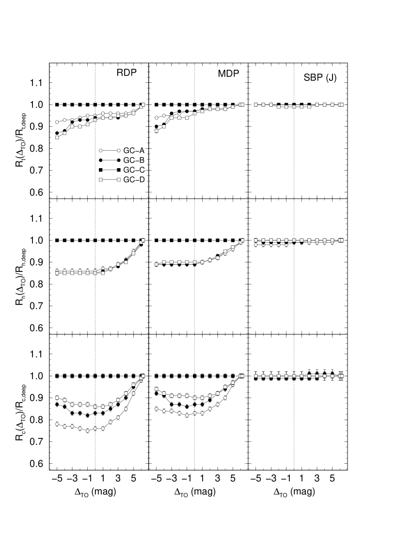
Figure 3: Structural parameters of the GC models. Top panels: Ratio of the tidal radius measured in profiles with a photometric depth $\rm\Delta_{TO}$ with respect to that derived from the deepest one, for the RDPs (left panels), MDPs (vertical-middle) and SBPs (right). Horizontal-middle panels: half-type radii. Bottom: core radii. TO values are indicated by the dotted line. Except for GC-C (uniform mass function), the remaining models present changes in radii in the RDPs and MDPs. SBP radii are essentially uniform.

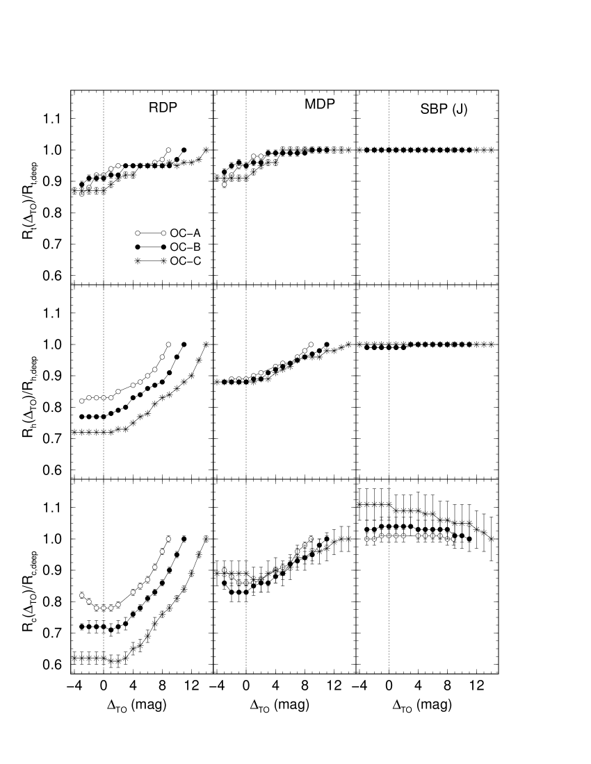
Figure 4: Same as Fig. 3 for the OC models. For comparison purposes, the y-scale is the same as in Fig. 3. Similarly to the GC models, radii changes are conspicuous in the RDPs and MDPs.

3 Structural parameters vs. photometry depth

The depth-varying model SBPs are fit with the empirical three-parameter function introduced by King (1962) to describe the surface-brightness distribution of GCs, which is characterised by the presence of the core and tidal radii. For RDPs and MDPs we use the King-like analytical profile that describes the projected number-density of stars as a function of $\rm R_{c}$ and $\rm R_{t}$, $\sigma(R)=\frac{dN}{2\pi\,R\,dR}$, as given by eq. 1. We also compute the distances from the center which contains half of the cluster’s total light, stars and mass. The half-star count ($\rm R_{hSC}$), light ($\rm R_{hL}$) and mass ($\rm R_{hM}$) radii are derived by directly integrating the corresponding profiles.

A selection of the resulting structural parameters as a function of $\rm\Delta_{TO}$ is given in Table 2. For simplicity we only present the values obtained from the bright and faint magnitude ranges, as well as for $M_{J}\leq M_{J,TO}$. The whole set of parameters are contained in Figs. 3 - 6. At first glance, RDP and MDP radii present a significant decrease for shallower photometry, with respect to the intrinsic values. SBP radii, on the other hand, are more uniform. The most noticeable feature is that, except for GC-C (uniform mass function), RDP and MDP radii tend to become increasingly larger than SBP ones with increasing photometric depth.

3.1 Dependence on photometric depth

In Fig. 3 we compare the radii measured in GC profiles built with a given photometric depth (e.g. $\mbox{$\rm R_{c}$}(\Delta_{TO})$) with the intrinsic ones, i.e. those derived from the deepest profiles ($R_{c,deep}$). RDP parameters are more affected than the MDP ones, while the SBP ones are essentially uniform, thus insensitive to photometric depth. Among the radii, RDP and MDP core are the most affected (underestimated), followed by the half and tidal radii. In the most concentrated model (GC-A, $c\approx 0.7$), measurements or $\rm R_{c}$ in the RDP may be underestimated by a factor $\approx 25\%$ in profiles shallower than near the TO, with respect to $R_{c,deep}$, and $\approx 20\%$ in MDPs. The effect is smaller in $\rm R_{hSC}$ and $\rm R_{hM}$, which may be underestimated by $\approx 15\%$ in the same profiles. The underestimation in the tidal radii is smaller than $\approx 10\%$. As expected, RDP, MDP and SBP radii do not change when the mass function is uniform (GC-C model).

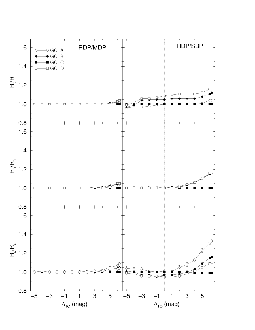
Figure 5: GC model profiles. Ratio between the same type of radii as measured in RDPs and MDPs (left panels) and RDPs and SBPs (right panels). From top to bottom: tidal, half and core radii. TO values are indicated by the dotted line.

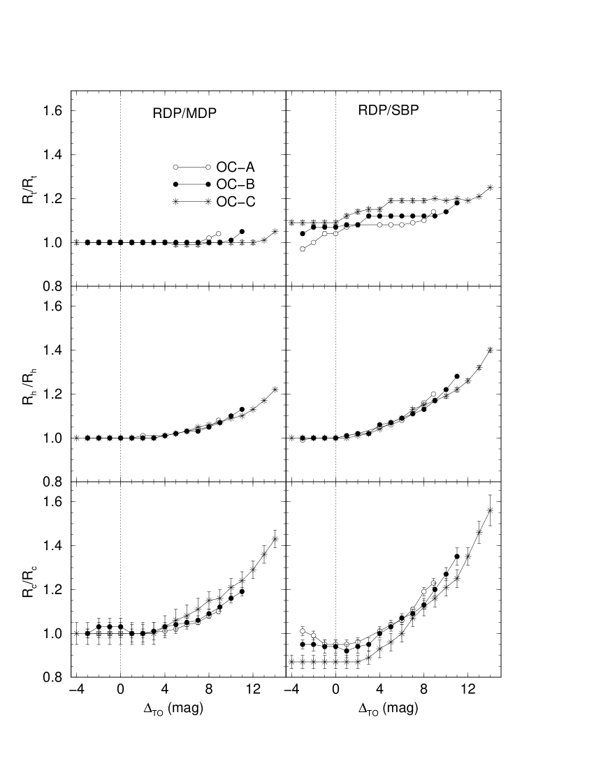
Figure 6: Same as Fig. 5 for the OC models. For comparison purposes, the y-scale is the same as in Fig. 5.

Similar radii ratios in the OC models are examined in Fig. 4. Qualitatively, the same conclusions drawn from the GC models apply to the OC ones. However, the underestimation factor of RDP radii increases for younger ages, to the point that $\rm R_{c}$ drops to $\approx 60\%$ of the deepest value for all profiles shallower than $\approx 3$  mag below the TO in the OC-C model ($10$ Myr), and to $\approx 70\%$ for OC-B ($100$ Myr). The respective half-star count radii are affected by similar, although smaller, underestimation factors. MDP radii are less affected by cluster age than RDP ones. Similarly to the GC models (Fig. 3), the three types of SBP radii are essentially insensitive to photometric depth, within uncertainties. We note that the presence of bright stars in the central region of young clusters (OC-C) appears to introduce a small dependence of the core radius on photometric depth (bottom-right panel).

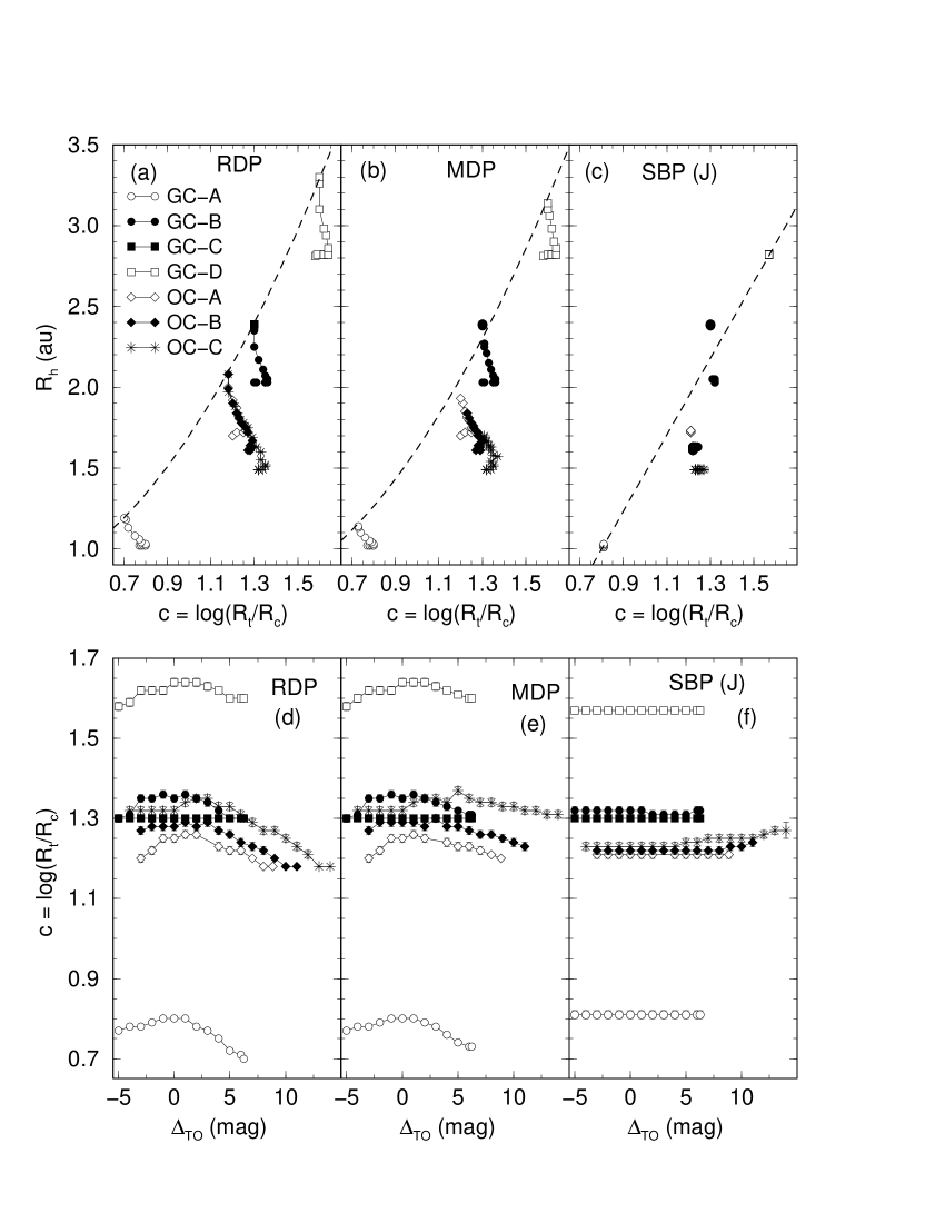
Figure 7: Top panels: relation of the half-type radii with the concentration parameter, for the RDPs (left panel), MDPs (middle) and SBPs (right). For each model, $R_{h}$ values increase for deeper profiles. Dashed line in panels (a) and (b): $R_{h}\sim c^{2}$. In panel (c): $\mbox{$\rm R_{hL}$}\sim c$. Bottom panels: concentration parameter as a function of photometric depth.

3.2 Comparison of similar radii among different profiles

Differences on the same type of radii among the profiles, introduced essentially by a spatially variable MF, are discussed in Fig. 5 for the GC models. Regardless of the model assumptions, RDP and MDP radii are essentially the same, except for the profiles corresponding to deep photometry, for which the RDP radii become slightly larger than the MDP ones. This occurs basically because of the larger fraction of low-mass stars at the outer parts of the clusters. Since all stars have equal weight in the building of the RDPs, the accumulation of low-mass stars at large radii ends up broadening the RDPs with respect to the MDPs. On the other hand, RDP core and half-star count radii tend to be larger than the SBP ones for profiles including stars fainter than near the TO. RDP $\rm R_{t}$ may be 10 – 20% larger than SBP ones for all depths. As discussed above, the uniformly-depleted MF of GC-C model produces profiles whose radii are independent of photometry depth. The RDP to SBP core and tidal radii ratios decrease with concentration parameter. The RDP to SBP half-type radii ratios do not depend on $c$.

The same analysis applied to the OC models is discussed in Fig. 6. The presence of massive stars in young clusters enhances the RDP to MDP radii ratios, especially the core and to some extent, the half-type radii. This occurs for profiles that contain stars brighter than $\approx 4$ mag below the TO. For the youngest model (OC-C), the core radius measured in the RDP may be $\approx 40\%$ larger than the MDP one. This effect is enhanced when RDP radii are compared to SBP ones, again decreasing in intensity from the core to tidal radii. For OC-C, RDP core, half and tidal radii are $\approx 55\%$, $\approx 40\%$, and $\approx 25\%$ larger than the equivalent SBP ones. Comparing with the GC models (Fig. 5), the presence of a larger fraction of more massive (brighter) stars towards the center in young clusters tend to enhance radii ratios of RDP with respect to MDP, and especially, RDP to SBP.

3.3 Further relations

The models discussed in previous sections can be used as well to examine the dependence of the half-type radii with the concentration parameter, and to test how $c$ varies with photometric depth. These issues are presented in Fig. 7.

As already suggested by Figs. 3 and 4, the relation of the half radius with $c$, in a given model, changes significantly with photometric depth in RDPs (panel a) and MDPs (panel b). In SBPs, on the other hand, it is almost insensitive to depth (panel c). From eq. 1, the half-star count radius is tightly related to the concentration parameter according to $\mbox{$\rm R_{hSC}$}=(0.69\pm 0.01)+(1.01\pm 0.01)\,c^{2}$. This curve fits well the values measured in the deepest RDP of all GC and OC models alike (panel a). Such a relation fails for the shallower profiles. A similar, but poorer, relation applies to the values derived from the deepest MDPs (panel b), $\mbox{$\rm R_{hM}$}=(0.63\pm 0.09)+(0.99\pm 0.05)\,c^{2}$. It fails especially for the young (OC) models. The GC SBPs, on the other hand, can be poorly fit with the linear function $\mbox{$\rm R_{hL}$}=(-0.9\pm 0.1)+(2.4\pm 0.1)\,c$ (panel c).

Concentration parameters measured in RDPs and MDPs (panels d and e) change with photometric depth. Around the TO they reach the maximum value, which corresponds to a star cluster $\approx 15\%$ more concentrated than the pre-established value (Table 1). At the shallowest profiles $c$ presents a value intermediate between the maximum and the pre-established one, which is retrieved at the deepest profiles with the inclusion of the numerous low-mass stars. The exception again is the uniform MF model GC-C, whose $c$ values do not change with $\Delta_{TO}$. $c$ values measured in SBPs are essentially insensitive to photometric depth (panel f).

4 NGC 6397: a test case

We compare the results derived for the model star clusters with similar parameters measured in the $\mbox{$\rm M_{V}$}=-6.63$, nearby GC ($\mbox{$\rm d_{\odot}$}=2.3$ kpc) NGC 6397. Being populous is important to produce statistically significant radial profiles, while the proximity allows a few magnitudes fainter than the giant branch to be reached with depth-limited photometry.

NGC 6397 is a post-core collapse GC with evidence of large-scale mass segregation, as indicated by a mass function flatter at the center than outwards (Andreuzzi et al. 2004 and references therein).

Additional relevant data (from H03) for the metal-poor ($\mbox{$\rm[Fe/H]$}=-1.95$) GC NGC 6397 are the Galactocentric distance $\mbox{$\rm R_{GC}$}=6$ kpc, half-light and tidal radii (measured in the V band) $\mbox{$\rm R_{hL}$}=2.33\arcmin$ and $\mbox{$\rm R_{t}$}=15.81\arcmin$, and Galactic coordinates $\ell=338.17^{\circ}$, $b=-11.96^{\circ}$. Thus, bulge star contamination is not heavy, and cluster sequences can be unambiguously detected, which is important for the extraction of radial profiles with small errors (see below). Using SBPs built with 2MASS images and a fit with King (1962) profile, Cohen et al. (2006) derived the core radius in the $\rm J$ band $\mbox{$\rm R_{c}$}(J)=61.5\arcsec\pm 9.3\arcsec$. However, based on Hubble Space Telescope data and using a power-law plus core as fit function, Noyola & Gebhardt (2006) derived $\mbox{$\rm R_{c}$}=3.7\arcsec$ in the equivalent V band, thus roughly resolving the post-core collapse nucleus.

The post-core collapse state of NGC 6397 does not affect the present analysis, since the goal here is the determination of changes produced in cluster radii derived under the assumption of a King-like profile (Sect. 3) applied to RDP, MDP and SBPs built with different magnitude depths. We base the analysis of NGC 6397 on $\rm J$, $\rm H$ and $\rm K_{s}$ 2MASS photometry extracted using VizieR in a circular field of radius $\mbox{$\rm R_{ext}$}=70\arcmin$ centered on the coordinates provided in H03. This extraction radius is large enough to encompass the whole cluster, allowing as well for a significant comparison field.

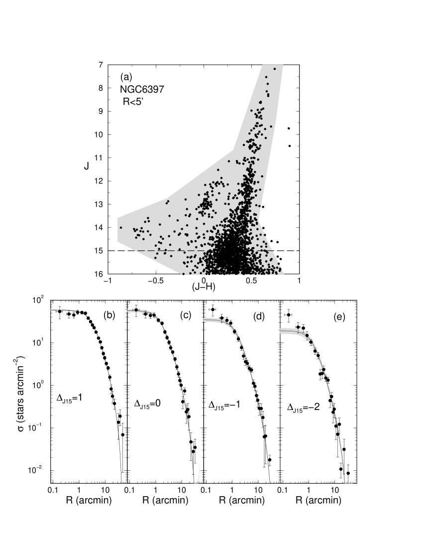
Figure 8: Structural analysis of NGC 6397. Panel (a): decontaminated CMD of a central ($R<5\arcmin$) region. The reference magnitude $\mbox{$\rm J$}=15$ is indicated by the dashed-line. Shaded region: colour-magnitude filter. Background-subtracted RDPs for stars brighter than $\mbox{$\rm J$}<15+\Delta_{J15}$, with $\Delta_{J15}=1,\leavevmode\nobreak\ 0,\leavevmode\nobreak\ -1,\leavevmode\nobreak\ -2$ are shown in panels (b) to (d), respectively. The respective King-like fits (solid-line) together with the fit uncertainty (shaded region) are shown.

For a better definition of the cluster sequences we apply the statistical decontamination algorithm described in Bonatto & Bica (2007), which takes into account the relative number-densities of candidate cluster and field stars in small cubic CMD cells with axes corresponding to the magnitude $\rm J$ and the colours $\rm(J-H)$ and $\rm(J-K_{s})$. Basically, the algorithm (i) divides the full range of magnitude and colours of the CMD into a 3D grid, (ii) computes the expected number-density of field stars in each cell based on the number of comparison field stars with magnitude and colours compatible with those in the cell, and (iii) subtracts the expected number of field stars from each cell. Typical cell dimensions are $\Delta\mbox{$\rm J$}=0.5$, and $\Delta\mbox{$\rm(J-H)$}=\Delta\mbox{$\rm(J-K_{s})$}=0.25$, which are large enough to allow sufficient star-count statistics in individual cells and small enough to preserve the morphology of the CMD evolutionary sequences. The comparison field is the region located between $50\leq R(\arcmin)\leq 70$, which is beyond the tidal radius.

Field-decontaminated CMDs allow for a better definition of colour-magnitude filters, useful to remove stars (and artifacts) with colours compatible with those of the field which, in turn, improves the cluster/background contrast in RDPs and SBPs. They are wide enough to accommodate cluster MS and evolved star colour distributions and dynamical evolution-related effects, such as enhanced fractions of binaries and other multiple systems (e.g. Bonatto & Bica 2007; Bonatto et al. 2005).

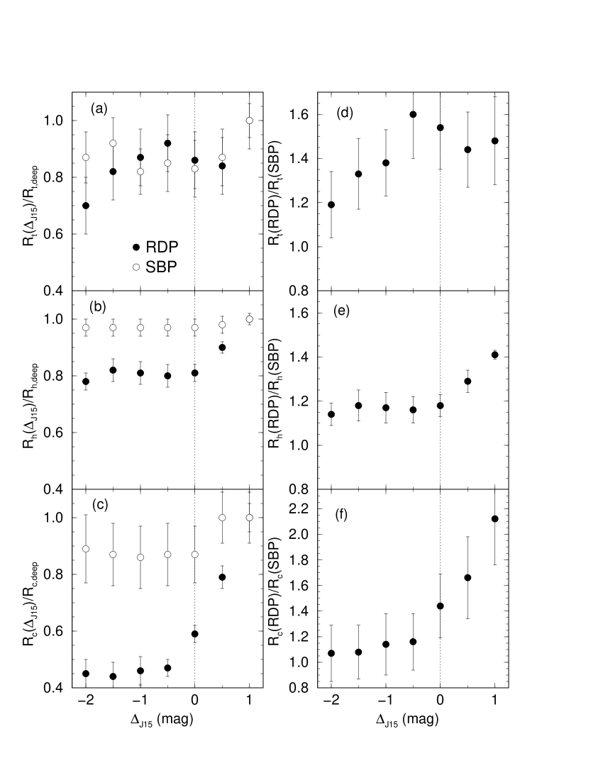
Figure 9: Left panels: RDP and SBP structural radii of NGC 6397 as a function of $\Delta_{J15}$, normalised to the values measured in the deepest profile. Right panels: RDP to SBP radii ratios (similar to Fig. 5).

Figure 8 (panel a) displays the decontaminated CMD of a central region of NGC 6397, with $R<5\arcmin$, somewhat larger than the half-light radius (Table 3). We take $\mbox{$\rm J$}=15$ as reference to extract the depth-variable profiles. RDPs and SBPs are built with colour-magnitude filtered photometry, with the faint end varying in steps of $\Delta_{J15}=0.5$, with the deepest (i.e. at the available 2MASS depth) profile beginning at $\mbox{$\rm J$}=16$ and the brightest one ending near the giant clump at $\mbox{$\rm J$}=13$. The extracted profiles are fitted with the King-like function discussed in (Sect. 2). A selection of depth-limited RDPs, together with the respective fits and uncertainties, is shown in Fig. 8, and the corresponding RDP and SBP ($\rm J$ band) radii are given in Table 3. Within uncertainties, the present value of the core radius (for the deepest profile), $\mbox{$\rm R_{c}$}(\mbox{$\rm J$})=1.4\arcmin\pm 0.3\arcmin$, agrees with that derived by Cohen et al. (2006), using the same fit function. The near-infrared half-light radius, on the other hand, is larger than the optical one (H03), $\mbox{$\rm R_{hL}$}(\mbox{$\rm J$})\approx 1.5\mbox{$\rm R_{hL}$}(V)$.

Effects of the varying magnitude depth on the radii of NGC 6397 are examined in Fig. 9. Qualitatively, the resulting curves agree, within uncertainties, with the behaviour predicted by the GC models (Figs. 3 and 5). Compared to the values measured in the deepest RDP, the tidal (panel a), half-star counts (b) and core (c) radii decrease for shallower profiles, especially for $\Delta_{J15}\geq-0.5$, remaining almost uniform for $\Delta_{J15}<-0.5$. In particular, the core radius measured in shallow RDPs (containing essentially giants) drops to $\approx 45\%$ of its deepest value (which includes stars at the top of the MS). Consistently with the GC models containing a spatially variable MF (Sect. 3), the varying depth affects the tidal, half and core radii, with increasing intensity. SBP radii, on the other hand, remain essentially uniform with variable depth, consistent with the GC models (Sect. 3). The same conclusions apply to the RDP to SBP radii ratio (right panels).

Table 3: Radii of NGC 6397 from RDPs and 2MASS SBPs

	RDP			SBP ($\rm J$ band)
$\Delta_{J15}$	$\rm R_{c}$	$\rm R_{hSC}$	$\rm R_{t}$	$\rm R_{c}$	$\rm R_{hL}$	$\rm R_{t}$
(mag)	(′)	(′)	(′)	(′)	(′)	(′)
(1)	(2)	(3)	(4)	(5)	(6)	(7)
$-2.0$	$1.3\pm 0.1$	$3.8\pm 0.1$	$33\pm 5$	$1.2\pm 0.3$	$3.4\pm 0.1$	$28\pm 5$
$-1.5$	$1.3\pm 0.1$	$4.0\pm 0.2$	$39\pm 8$	$1.2\pm 0.3$	$3.4\pm 0.1$	$30\pm 5$
$-1.0$	$1.3\pm 0.1$	$4.0\pm 0.2$	$42\pm 8$	$1.2\pm 0.3$	$3.4\pm 0.1$	$26\pm 5$
$-0.5$	$1.4\pm 0.1$	$3.9\pm 0.2$	$44\pm 7$	$1.2\pm 0.3$	$3.4\pm 0.1$	$27\pm 8$
$\leavevmode\nobreak\ 0.0$	$1.7\pm 0.1$	$4.0\pm 0.1$	$41\pm 4$	$1.2\pm 0.3$	$3.4\pm 0.1$	$27\pm 6$
$+0.5$	$2.3\pm 0.1$	$4.4\pm 0.1$	$40\pm 4$	$1.4\pm 0.4$	$3.4\pm 0.1$	$28\pm 8$
$+1.0$	$2.9\pm 0.1$	$4.9\pm 0.1$	$48\pm 3$	$1.4\pm 0.3$	$3.5\pm 0.1$	$32\pm 2$

• Core and tidal radii were derived from fits of King (1962) functions (Sect. 3) to the respective profiles. The half-star counts and half-light radii were measured directly on the profiles.

5 Concluding remarks

In this work we simulated star clusters of different ages, structure and mass functions, assuming that the spatial distribution of stars follows an analytical function, similar to King (1962) profile. The mass and near-infrared luminosities of each star were assigned according to a mass function with a slope that may depend on distance to cluster center. They form the set of models from which we built number-density, mass-density and surface-brightness profiles, allowing for a variable photometric depth. The structural parameters core, half-light, half-mass and half-star count, and tidal radii, together with the concentration parameter, were measured in the resulting radial profiles. Next we examined relations among similar parameters measured in different profiles, and determined how each parameter depends on photometric depth. We point out that the results should be taken as upper-limits, especially for open clusters, since we have considered noise-free photometry and a large number of stars, which produced small statistical uncertainties.

With respect to the adopted form of the radial distribution of stars, we note that King (1962) isothermal sphere, single-mass profile has been superseded by more realistic models like those of King (1966), Wilson (1975) and Elson et al. (1987), which have been fit mostly to the SBPs of Galactic and extra-Galactic GCs (Sect. 2). The analytical functions associated with these models are characterised by different scale radii (among other parameters) that are roughly related to King (1962) radii. Thus, it is natural to extend the scaling with photometric depth undergone by King (1962) radii to the equivalent ones in the other models.

The main results can be summarised as follows.

• (i) Structural parameters derived from surface-brightness profiles are essentially insensitive to photometric depth, except perhaps the cluster radius in very young clusters.

• (ii) Uniform mass functions also result in structural parameters insensitive to photometric depth.

• (iii) Number-density and mass-density profiles built with shallow photometry result in underestimated radii, with respect to the values obtained with deep photometry. Tidal, half-star count and half-mass, together with the core radii are affected with increasing intensity.

• (iv) Because of the presence of bright stars, radii underestimation increases for young ages.

• (v) For clusters older than $\sim 1$ Gyr, number-density and mass-density radii present essentially the same values; for younger ages, RDP radii become increasingly larger than MDP ones, especially at the deepest profiles.

• (vi) Irrespective of age, profiles deeper than the turnoff have RDP radii systematically larger than SBP ones, especially the core.

• (vii) The concentration parameter also changes with photometric depth, reaching a maximum around the turnoff.

Most of the above model predictions were qualitatively confirmed with radii measured in ground-based RDPs and SBPs of the nearby GC NGC 6397.

In principle, working with SBPs has the advantage of producing more uniform structural parameters, since they are almost insensitive to photometric depth. However, as discussed in Sect. 1, SBPs usually present high levels of noise at large radii. Noise that is also present in SBPs of clusters projected against dense fields and/or the less populous ones. A natural extension of this work would be to examine radial profiles built with photometry that includes observational uncertainties, differential absorption, metallicity gradients, binaries, and star cluster models with a number of stars compatible with those of open clusters.

As a consequence of the wide range of distances to the Galactic (and especially extra-Galactic) star clusters, interstellar absorption, and intrinsic instrumental limitations, the available photometric data for most clusters do not sample the low-mass stars. All sky surveys like 2MASS, usually are restricted to the giant branch, or the upper main sequence, for clusters more distant than a few kpc. In such cases, the structural parameters have to be derived from radial profiles built with photometry that does not reach low-mass stars. The present work provides a quantitative way to estimate the intrinsic (i.e. in the case of photometry including the lower main sequence) values of structural radii of star clusters observed with depth-limited photometry.

Appendix A Transformation of a random number distribution into an analytical function.

The simulations discussed in the present work depend on the transformation of a distribution of numbers $p(n)$, with $n$ varying in the range $0\leq n\leq 1$, into the analytical function $f(x)$, with $x$ in the range $x_{\rm min}\leq x\leq x_{\rm max}$. What results from this is that a random sorting of numbers $n$ would produce $x$ variables with a number-frequency given by the pre-defined function $f(x)$. Formally, the transformation is expressed as

$$f(x)\,dx=p(n)\,dn.$$ (5)

In a random distribution, all numbers have the same probability, so that we can set $p(n)=1$. Thus, the formal relation of $n$ to $x$ is given by

$$n(x)=\int_{x_{\rm min}}^{x}f(x^{\prime})\,dx^{\prime}/\int_{x_{\rm min}}^{x_{\rm max}}f(x^{\prime})\,dx^{\prime}.$$ (6)

The analytical (or numerical) inversion of the latter relation gives $x=x(n)$.

For example, consider a mass function $\phi(m)=\frac{dN}{dm}\propto m^{-(1+\chi)}$, with the mass varying in the range $m_{i}\leq m(\mbox{$\rm M_{\odot}$})\leq m_{s}$. If $\chi\neq 0.0$, what results from Eq. 6 is

$$n(m)=\left(m_{i}^{-\chi}-m^{-\chi}\right)/\left(m_{i}^{-\chi}-m_{s}^{-\chi}\right).$$

Solving this for $m$ produces

$$m(n)=m_{s}/[(1-n)(m_{s}/m_{i})^{\chi}+n]^{1/\chi}.$$

For $\chi=0.0$ the result is $m(n)=m_{i}\,(m_{s}/m_{i})^{n}$.

In the case of the three-parameter King-like profile (Eq. 1 in Sect. 2), the first step in the transformation, represented by Eq. 6, results in the $\rm n=n(R)$ function given by Eq. 2 (Sect. 2). However, the latter relation cannot be analytically inverted, so that this task has to be done numerically, using the curves plotted in Fig. 1 (panel a).