Quantum Blockade and Loop Currents in Graphene with Topological Defects

Abstract

We investigate the effect of topological defects on the transport properties of a narrow ballistic ribbon of graphene with zigzag edges. Our results show that the longitudinal conductance vanishes at several discrete Fermi energies where the system develops loop orbital electric currents with certain chirality. The chirality depends on the direction of the applied bias voltage and the sign of the local curvature created by the topological defects. This novel quantum localization phenomenon provides a new way to generate a magnetic moment by an external electric field, which can prove useful in nanotronics.

Graphene is a single layer of graphite with a honeycomb lattice consisting of two triangular sub-lattices. This peculiar structure of graphene gives rise to two linear ``Dirac-like'' energy dispersion spectra around two degenerate and inequivalent points $K$ and $K^{\prime}$ at the corner of the Brillouin zone Gon93 ; Kane05 . The valley index that distinguishes the two Dirac points is a good quantum number, even in the presence of weak disorder, since inter-valley scattering requires the exchange of large momentum. Valley-dependent physics has been actively explored recently and can potentially play an important role in future graphene based devices Ryc07 ; Akh07 ; Niu07 .

To manipulate this extra degree of freedom, it is necessary to couple the two valleys. In graphene, there is a natural way to produce a valley coupling by creating topological defects such as pentagons and heptagons An01 . Such defects cannot be constructed from a perfect graphene sheet simply by replacing a hexagon by a pentagon or a heptagon. Instead, a ``cut-and-paste'' process Cor06 ; Sit07 should be employed to keep the local coordination number of each carbon atom, as illustrated in Fig. 1. A pentagon (heptagon) will induce a positive (negative) curvature around it. As can be observed from Fig. 1, after going around any closed carbon loop encircling the defect, which always consists of odd number of atoms, the roles of two sublattices are interchanged. Therefore, the defect breaks the bipartite nature of the lattice in the real space as well as the symmetry between the $K$ and $K^{\prime}$ points in reciprocal space, leading to a Möbius strip-like structure coupling the two valleys. Theoretically, the effect of topological defects on the low energy electric physics of graphene is equivalent to generating non-Abelian gauge potentials with the internal gauge group involving the transformation of valley index. The wave function acquires a topological phase when circling around the defect, which can be described by means of a non-Abelian gauge field. Experimentally, pentagon and heptagon topological defects have been found in graphite-related materials An01 ; Jas03 . In graphene, recently observed Nov04 ; Moro06 mesoscopic corrugations (ripples) are partially attributed to topological defects.

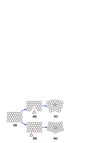
Figure 1: (color online) The process of constructing a pentagon ((a)$\rightarrow$(b) $\rightarrow$(c)) and a heptagon ((a)$\rightarrow$(d)$\rightarrow$(e)) by ``cut'' and ``paste'' from a perfect graphene sheet. Positive (negative) curvature is induced by a pentagon (heptagon) in the realistic three dimensional space. Notice that after the ``cut'' and ``paste'', a single pentagon (heptagon) will give rise to a global change of the lattice structure, which is explained in the text.

The equilibrium electronic properties of a two dimensional graphene in the presence of single or many topological defects have already received wide attention Cor06 ; Sit07 ; Lam00 ; Gon93 ; Char01 ; Ko00 ; Ta94 ; Ta97 . However, there is still much to understand about the transport properties of these systems. In this paper, we investigate the electronic transport properties of a zigzag edge graphene nanoribbon with several topological defects: a pentagon, a heptagon, and a pentagon-heptagon pair at the center. We numerically calculate the total conductance $G$ and the spatial distribution of local currents $i(\mathbf{r})$. We reveal a novel quantum localization phenomenon whereby the conductance vanishes at discrete Fermi energies in the first quantized plateau. This effect is accompanied by the development of circular loop currents with prescribed chirality, owing their existence to the non-Abelian gauge potentials connecting the valleys. The chirality depends on both the direction of the applied bias voltage and the sign of curvature created by topological defects, and can hence be easily controlled and manipulated. The result opens a new possibility to generate magnetic moments by an external electric field in graphene.

The $\pi$ electrons in graphene are modeled by the tight binding spinless Hamiltonian

$$H_{G}=\sum_{i}\epsilon_{0}c_{i}^{\dagger}c_{i}+t\sum_{\langle i,j\rangle}(c_{i}^{\dagger}c_{j}+\text{H.c}),$$ (1)

where $c_{i}^{{\dagger}}$ ($c_{i}$) creates (annihilates) an electron on site $i$, $\varepsilon_{0}$ (set to 0) is the on-site energy and $t$ ($\sim$2.7eV) is the hopping integral between the nearest neighbor carbon atoms separated by $a$ ($\sim$1.42Å). $t$ and $a$ are used as the energy unit and the length unit, respectively. The hopping $t$ is taken to be constant for all the C-C bonds, even those on the defect. Small changes of the hopping integral $t$ due to orbital mixing from the curvature Klein01 are neglected since they do not generate large momentum scattering, which means that pure topological effects are considered.

The zero temperature two terminal conductance $G$ of the sample and local density of states (LDOS) $\rho_{m}$ of site $m$ at Fermi energy $E_{F}$ are given by Datta

$$G(E_{F}) = \frac{2e^{2}}{h}\text{Tr}(\Gamma_{S}(E_{F})G^{r}(E_{F})\Gamma_{D}(E_{F})G^{a}(E_{F})),$$ (2)

$$\rho_{m}(E_{F}) = -\frac{1}{\pi}\text{Im}[G_{m,m}^{r}(E_{F})],$$ (3)

where $G^{r(a)}(E_{F})=(E_{F}-H_{G}-\Sigma_{S}^{r(a)}(E_{F})-\Sigma_{D}^{r(a)}(E_{F}))^{-1}$ is the retarded (advanced) Green's function, $G^{a}(E_{F})=(G^{r}(E_{F}))^{\dagger}$, $\Gamma_{S(D)}(E_{F})=i[\Sigma_{S(D)}^{r}(E_{F})-\Sigma_{S(D)}^{a}(E_{F})]$, $H_{G}$ is the Hamiltonian of the graphene sample and $\Sigma_{S}^{r(a)}\equiv H_{GS}G^{r(a)}_{S}H_{SG}=H_{GS}(E_{F}\pm i\eta-H_{S})^{-1}H_{SG}$ is the retarded (advanced) self-energy due to the semi-infinite source, and the self-energy due to the drain $\Sigma_{D}^{r(a)}$ is similar. The self-energies can be numerically calculated in a recursive way Lee ; JZhang . We attach clean graphene as source and drain leads to avoid redundant scattering from mismatched interfaces between the sample and the leads.

The current per unit energy at the Fermi level $E_{F}$ between neighboring sites $m$ and $n$ is Datta ; Naka01 ; Anan07 ; Guo04

$$i_{m\rightarrow n}(E_{F}) = \frac{4e}{\hbar}\langle\text{Im}[\psi_{m}^{*}t\psi_{n}]\rangle=\frac{4e}{\hbar}\langle H_{mn}|\psi_{m}||\psi_{n}|\sin(\theta_{n}-\theta_{m})\rangle$$ (4)

$$= \frac{4e}{h}\text{Im}[H_{mn}G^{n}_{n,m}(E_{F})],$$ (5)

where $\psi_{m}$ is the amplitude of the wave function at site $m$, $G^{n}\equiv G^{R}(\Gamma_{S}f(\mu_{S})+\Gamma_{D}f(\mu_{D}))G^{A}$ is the electron correlation function and $f$ is the Fermi distribution function, $\theta_{n}$ is the phase of $\psi_{n}$ and $H_{mn}\equiv t$. The quantum current $i$ contains information about the phase shift of wave functions between the neighboring sites.

The local current $I_{m\rightarrow n}$ is the energy integral of $i_{m\rightarrow n}$:

$$I_{m\rightarrow n} = \int^{\mu_{S}}_{-\infty}i_{m\rightarrow n}(E)dE$$ (6)

$$= \int^{\mu_{S}}_{\mu_{D}}\frac{4et}{h}\text{Im}[G^{R}(E)\Gamma_{S}(E)G^{A}(E)]_{mn}dE\quad\textrm{\Big{(}zero temperature and zero magnetic field\Big{)}}$$ (7)

$$= i_{m\rightarrow n}(\mu_{S})eV_{b}\quad\textrm{\Big{(}linear response limit \Big{)}}$$ (8)

where the bias $V_{b}$ is related to the source (drain) chemical potential $\mu_{S}$ ($\mu_{D}$) by $\mu_{S}-\mu_{D}=eV_{b}$. Equation (7) can be derived from equation (5) in a straightforward way along with the fact that Green's functions are symmetric matrices in the absence of magnetic field and thermal fluctuations, thus the contributions below $\mu_{D}$ cancel, making the local current a Fermi surface property Datta .

We constructed a pentagonal defect in the center of a zigzag edge graphene sheet with $45\times 20$ sites. in the presence of the pentagon, as shown in Fig. 2, the conductance $G$ is suppressed by defect scattering in most regions of energy compared to the quantized conductance Peres06 of the ballistic case. The $G(E)$ curves exhibit dips and kinks at some special energy points. The details of these points are the main focus of this work.

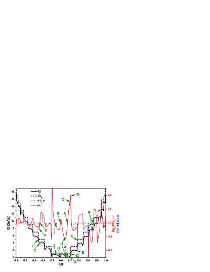
Figure 2: (color online) Conductance of the topologically disordered sample with a pentagon $G$ (black solid), averaged loop current $\langle i_{L}\rangle$ (blue dashed dot) and induced magnetic moment $m$ (red solid) of the pentagon as functions of Fermi energy $E$. The conductance for a perfect graphene sample $G_{0}$ (black dashed) with the same dimensions is also plotted for reference.

Let us first concentrate on the dips A and B in Fig. 2, where the conductance is reduced by the amount of $g_{0}=2e^{2}/h$, suggesting a single conducting channel at this energy has been completely blocked. The local shape of the dips is approximately Lorentzian. An anti-resonance with such features has been observed in one-dimensional (1D) systems with topological defects Louie00 ; Guin87 ; Wang02 . The location of these anti-resonances is not universal, but is determined by the topological configuration of the lattice and its defects. Unlike the 1D case, the locations of these anti-resonances do not have a simple relation with the energy levels of the defect or the sample. The multi-dimensional nature of the transmission matrix and the inter-channel scattering make an analytical treatment more complicated. However, the physical result is the same as that in 1D. The phenomenon at hand can be called topological quantum localization.

To gain better insight in the microscopic origins of the localization, we plot, in Fig. 3 (a) and (b), the spatial distribution of LDOS $\rho$, and local currents $i$ far (point J in Fig. 2) away from and near (point H in Fig. 2) the antiresonance respectively. The LDOS does not vary much at the two points, but the currents do. In Fig. 3 (a), where $G$ is not sharply suppressed, the spatial distribution of $i(\mathbf{r})$ is rather uniform, and almost all of the bond currents flow from the source (right) to the drain (left). On the contrary, in Fig. 3 (b), loop currents flow circularly around the defect in the same direction, giving rise to a vortex-like pattern of local currents. Interestingly, these loop currents reverse their chirality when the Fermi energy is swept from one side to the other side of the antiresonance, as can be seen in Fig. 3 (c). The magnitude of the current on the pentagon bonds may be larger than the source-drain current. Moreover, loop currents on some of the hexagons in the proximity of the defect can also be observed. This is a quantum effect, which is forbidden in a classical resistance network Altshuler , due to the lack of an external battery or magnetic field on the loops. This pattern exhibits almost perfect five-fold rotation symmetry of the pentagon. Since the graphene sample used here lacks the rotational symmetry of the pentagon, the pattern in Fig. 3 (b) does not originate from an artificial symmetric arrangement of the device, but is an intrinsic property of the topological defect, and can be expected to exist in the realistic system. In the case of an infinite graphene sheet, the first conductance plateau containing this bounding state encircling the defect degenerates into the Dirac point. The existence of this bounding state at Dirac point is consistent with previous predictions based on the the continuum description of 2D graphene Cor06 ; Lam00 ; Sit07 .

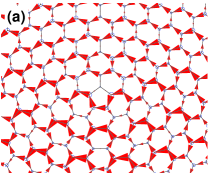
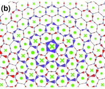
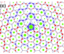
Figure 3: (color online) The spatial distribution of LDOS of the sites (blue circles), local current density of the bonds (arrows) and induced magnetic moment of carbon rings (green disks and crosses) near the pentagon. The size of each symbol is proportional to the local value of the corresponding quantity. (a) $E=-0.1t$, corresponding to point J in Fig. 2, far away from the anti-resonance. (b) $E=0.1t$, corresponding to point H in Fig. 2, near the anti-resonance. (c) $E=0.2t$, corresponding to point Q in Fig. 2, on the other side of the anti-resonance. Some circular loop currents around the pentagon are stressed in purple arrows. Note that circular loop currents can also be observed on some hexagons near the defect.

The vortex-like loop currents suggest that the topological defect introduces an effective magnetic field Wakabayashi , which is consistent with theoretical predictions Lam00 ; Cor06 ; Sit07 . According to (5), the loop currents reflect the peculiar phase correlation induced by the topological defect. Given a closed carbon loop, we define the bond current on the loop as positive if it points clockwise, and negative otherwise. Thus the averaged loop current (ALC) density $\langle i_{L}\rangle_{\text{loop}}$ of a closed loop can be defined as

$$\langle i_{L}\rangle_{\text{loop}}=\frac{1}{N}\theta(i_{\text{max}}\cdot i_{\text{min}})\cdot\sum_{\langle k,l\rangle\in\text{loop}}i_{k\rightarrow l},$$ (9)

where $N$ is the number of bonds (also the number of sites) on the loop, $\theta(x)$ is the Heaviside step function, and $i_{\text{max}}$ ($i_{\text{min}}$) is the maximum (minimum) current on the loop. Obviously a current on the loop can be called ``circular'' only if $i_{\text{max}}\cdot i_{\text{min}}>0$, so that $\langle i_{L}\rangle_{\text{loop}}\neq 0$. The induced magnetic moment density on a closed loop is expressed as Naka01

$$\mathbf{m}_{\text{loop}}(E)=\sum_{\langle k,l\rangle\in\text{loop}}i_{k\rightarrow l}(E)(\mathbf{r}_{k}\times\mathbf{r}_{l})/2,$$ (10)

where $\mathbf{r}_{k}$ is the coordinates of the site $k$. A relation similar to that of $I$ and $i$ in (7 and 8) holds between the magnetic moment $\mathbf{M}$ and its energy density $\mathbf{m}$. Due to equations (7) and (8), we simply discuss the densities $i$ and $\mathbf{m}$ in the following, but refer to them simply as current and magnetic moment. The ALC and magnetic moment as functions of energy are plotted in Fig. 2. They change signs when energy crosses an anti-resonance (A and B in Fig. 2). This is an important correlation between the magnetic moment direction and the anti-resonances.

We also note that at the edges of quantized conductance plateau (edges of sub-bands also), such as at the points D, E, and F in Fig. 2, the conductance has a kink-like or a dip-like behavior. This enhanced scattering was also observed in disordered graphene with non-topological impurities Zhang07 , and can be attributed to extreme level-broadening (or velocity renormalization) due to van Hove singularity at the sub-band edges QTD . As can be seen from Fig. 2, this enhanced scattering is also accompanied by a (qusi-) loop current on the defect, albeit with different behavior from the purely topological localization previously discussed: the directions of $\langle i_{L}\rangle_{\text{pentagon}}$ and/or $\langle m\rangle_{\text{pentagon}}$ are singly-polarized near the conductance dip or peak, while the magnitude has a sharp peak.

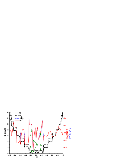
Figure 4: (color online) Conductance of the topologically disordered sample with a heptagon $G$ (black solid), averaged loop current $\langle i_{L}\rangle$ (blue dashed dot) and induced magnetic moment $m$ (red solid) of the pentagon as functions of Fermi energy $E$. The conductance for a perfect graphene sample $G_{0}$ (black dashed) with the same dimensions is also plotted for reference.

The transport properties of graphene with a single heptagon are also analyzed. Fig.4 and Fig.5 are the results for constructing a heptagonal defect in the center of a zigzag edge graphene sheet with $30\times 16$ sites. The quantum localizations, vortex-like loop currents around the defect and reversal of the chirality across the anti-resonance can also be observed, except the pattern of loop currents now has seven-fold rotationally symmetry.

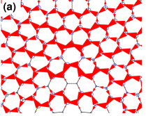
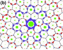
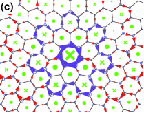
Figure 5: (color online) The spatial distribution of LDOS of the sites (blue circles), local current density of the bonds (arrows) and induced magnetic moment of carbon rings (green disks and crosses) near the heptagon. The size of each symbol is proportional to the local value of the corresponding quantity. (a) $E=0.17t$, corresponding to point A in Fig. 4, far away from the anti-resonance. (b) $E=-0.15t$, corresponding to point B in Fig. 4, near the anti-resonance. (c) $E=-0.12t$, corresponding to point C in Fig. 4, on the other side of the anti-resonance. Some loop currents around the pentagon are stressed in purple arrows. Note that circular loop currents can also be observed on some hexagons near the defect.

We now consider the pentagon-heptagon at the center of graphene. With almost zero curvature, this is believed to be a stable configuration in carbon-related materials. In Fig. 6, the conductance $G$, the ALCs $\langle i_{L}\rangle_{\text{pentagon}}$ and $\langle i_{L}\rangle_{\text{heptagon}}$ are plotted. Within the first conductance plateau, the anti-resonance only happens at the center and the edges of the plateau, and $\langle i_{L}\rangle_{\text{pentagon}}$ and $\langle i_{L}\rangle_{\text{heptagon}}$ always point in opposite directions. On the higher conductance plateaus, we observe different energy dependence of the two loop currents: non-zero loop current on the pentagon tends to appear for $E>0$ while it tends to appear for $E<0$ on the heptagon. This can be seen more clearly when we compare the local currents near the anti-resonance at negative (Fig. 7 (a)) and positive energy (Fig. 7 (b)), respectively. There are also vortex-like loop currents encircling the defect. When $E<0$, the magnitude of loop current on the heptagon is larger than that on the pentagon, and the loop currents encircling the whole defect have the same direction with the heptagon loop current(Fig. 7 (a)). Viceversa, when $E>0$, the magnitude of loop current on the pentagon is larger, and the vortex-like loop currents have the same direction with the pentagon loop current (Fig. 7 (b)). All these observations lead to a nontrivial conclusion that, when the pentagon-heptagon pair is present, the pentagon tends to trap the electronic motion in the positive energy region, while the heptagon is dominant in the negative energy region. The LDOS has a large magnitude on the defect, similar to the case of disordered carbon nanotubes Louie00 .

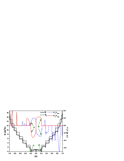
Figure 6: (color online) Conductance $G$ (black solid) of the topologically disordered sample with a pentagon-heptagon pair, averaged loop current of the pentagon $\langle i_{L}\rangle_{pen}$ (blue dashed dot) and the heptagon $\langle i_{L}\rangle_{hep}$ (red solid) as functions of Fermi energy $E$.

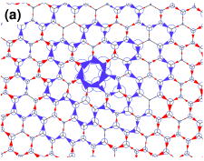
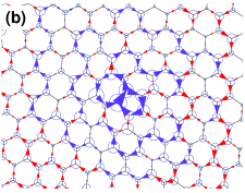
Figure 7: (color online) The spatial distribution of LDOS of the sites (blue circles), local current density of the bonds (arrows) near the pentagon-heptagon pair. (a) $E=-0.18t$, corresponding to point A in Fig. 6. (b) $E=0.2t$, corresponding to point B in Fig. 6. Some loop currents near the defect are plotted in purple arrows.

The quantum localization is realized only in the first quantized channel as the conductance never vanishes completely in higher conductance plateau (C and P in Fig. 2). In a graphene narrow ribbon with zigzag edges, the first quantized level is different from higher levels due to the presence of edge statesAkh07 . In the first quantized level, for a given Fermi level $E_{F}$, the currents carried in the states of one valley are rectified currents and the directions are opposite in different valleys. However, in the higher quantized levels, the states in each valley carry current in both directions. In the presence of the topological defects, the non-Abelian gauge potential scatters the states in one valley to states in the other valley. In the case of the first quantized level, the scattering can block the transport current and create the loop current, since the process reverse the current completely, while this is not the case in the high quantized levels.

It is interesting to compare our results with those of other carbon related structures. In Ref. Naka01 , a single C₆₀ molecule with discrete energy levels is connected to 1D leads, where pentagonal loop currents were discovered. While, in our work, the sample along with the leads is two-dimensional (2D) with continuous energy bands. Therefore, the role of the degenerate resonance level in Ref. Naka01 is quite analogous to that of the anti-resonance level here, where the loop currents reverse their directions. The perfect symmetry may be responsible for a much larger loop current in C₆₀ (several tens of $I_{SD}$) than in disordered graphene (few times of $I_{SD}$). Electronic transport through topologically disordered carbon nanotubes (CNTs) has been investigated Louie00 . But the topological defect therein should possess certain configuration to satisfy the periodic boundary condition in the transverse direction. Moreover, the circular motions of the electron was verified to play important roles in the transport, which is lacked in finite graphene ribbon with fixed boundary condition.

Before arriving at final conclusions, it is important to remark that, the understanding of bounding states associated with a single topological defect discussed here can be a starting point for investigating the effect of multiple topological defects. The interferences between the bounding states of the defects may give rise to some rich phenomena.

In conclusion, we have performed a numerical calculations of conductance and local currents for topologically disordered graphene with one pentagon, heptagon or pentagon-heptagon pair. A microscopic understanding of the conductance reduction is obtained. The strong scattering in these systems is always accompanied by (quasi-) loop currents around the defects. The chirality of the loop currents can be controlled by the bias voltage as well as the gate voltage near the discrete Fermi energies where quantum localization takes place. The magnetic moments generated by the loop currents can be measured in experiments, such as scanning tunneling microscope(STM) and Kerr effects. In the presence of the pentagon-heptagon pair defect, the pentagon (heptagon) is more likely to trap electrons with positive (negative) energy.

We thank Prof. F. Liu for discussions. This work is supported by RGC CERG603904, NSF of China under grant 90406017, 60525417, 10740420252, the NKBRSF of China under Grant 2005CB724508 and 2006CB921400. JPH is supported by the US-NSF (Grant No. PHY-0603759). XCX is supported by US-DOE and NSF.

References

- (1) J. González, F. Guinea and M. A. H. Vozmediano, Nuc. Phys. B406, [FS] 771 (1993).
- (2) C. L. Kane, Nature 438, 168 (2005).
- (3) A. Rycerz, J. J. Tworzydło and C. W. J. Beenakker, Nature Phys. 3, 172 (2007).
- (4) A. R. Akhmerov and C. W. J. Beenakker, Phys. Rev. Lett. 98, 157003 (2007).
- (5) D. Xiao, W. Yao and Q. Niu, Phys. Rev. Lett. 99, 236809 (2007).
- (6) B. An et al., Appl. Phys. Lett. 78, 3696 (2001).
- (7) A. Cortijo and M. A. H. Vozmediano, arXiv:cond-mat/0612374 (2006); Europhys. Lett. 77, 47002 (2007).
- (8) Y. A. Sitenko and N. D. Vlasii, arXiv:0706.2756 (2007).
- (9) J. A. Jaszczak et al., Carbon 41, 2085 (2003).
- (10) K. S. Novoselov et al., Science 306, 666 (2004) and SOM.
- (11) S.V. Morozov et al., Phys. Rev. Lett. 97, 016801 (2006).
- (12) R. Tamura and M. Tsukada, Phys. Rev. B 49, 7697 (1994).
- (13) P. E. Lammert and V. H. Crespi, Phys. Rev. Lett. 85, 5190 (2000).
- (14) J.-C. Charlier and G.-M. Rignanese, Phys. Rev. Lett. 86, 5970 (2001).
- (15) R. Tamura et al., Phys. Rev. B 56, 1404 (1997).
- (16) K. Kobayashi, Phys. Rev. B 61, 8496 (2000).
- (17) A. Kleiner and S. Eggert, Phys. Rev. B 64, 113402 (2001).
- (18) S. Datta, Electronic Transport in Mesoscopic Systems (Canmbridge University Press, Cambridge, U.K., 1995); S. Datta, Quantum Transport: Atom to Transistor (Canmbridge University Press, Cambridge, U.K., 2005).
- (19) D. H. Lee and J. D. Joannopoulos, Phys. Rev. B 23, 4997 (1981).
- (20) J. Zhang, Q. W. Shi and J. Yang, J. Chem. Phys. 120, 7733 (2004).
- (21) S. Nakanishi and M. Tsukada, Phys. Rev. Lett. 87, 126801 (2001).
- (22) Y. Liu and H. Guo, Phys. Rev. B 69, 115401 (2004).
- (23) M. P. Anantram, M. S. Lundstrom and D. E. Nikonov, arXiv:cond-mat/0610247V2 (2007).
- (24) N. M. R. Peres, A. H. Castro Neto and F. Guinea, Phys. Rev. B 73, 195411 (2006).
- (25) F. Guinea and J. A. Vergés, Phys. Rev. B 35, 979 (1987).
- (26) L. Chico, L. X. Benedict, S. G. Louie and M. L. Cohen, Phys. Rev. B 54, 2600 (1996); H. J. Choi, J. Ihm, S. G. Louie and M. L. Cohen, Phys. Rev. Lett. 84, 2917 (2000).
- (27) X. R. Wang, Y. P. Wang, and Z. Z. Sun, Phys. Rev. B 65, 193402 (2002).
- (28) V. V. Cheianov, V. I. Fal'ko, B. L. Altshuler and I. L. Aleiner, Phys. Rev. Lett. 99, 176801 (2007).
- (29) K. Wakabayashi and M. Sigrist, Phys. Rev. Lett. 84, 3390 (2000); K. Wakabayashi, Phys. Rev. B 64, 125428 (2001).
- (30) Y. Y. Zhang, J. P. Hu, X. C. Xie and W. M. Liu, arXiv:0708.2305 (2007).
- (31) T. Dittrich, P. Hänggi, G.-L. Ingold, B. Kramer, G. Schön and W. Zwerger, Quantum Transport and Dissipation (Wiley-VCH. 1998).