Flavour Physics and Grand Unification

Abstract

In spite of the enormous success of the Standard Model (SM), we have strong reasons to expect the presence of new physics beyond the SM at higher energies. The idea of the Grand Unification of all the known interactions in nature is perhaps the main reason behind these expectations. Low-energy Supersymmetry is closely linked with grand unification as a solution of the hierarchy problem associated with the ratio $M_{\mbox{\scriptsize GUT}}/M_{Z}$. In these lectures we will provide a general overview of Grand Unification and Supersymmetry with special emphasis on their phenomenological consequences at low energies. We will analyse the flavour and CP problems of Supersymmetry and try to identify in these associated low-energy observables possible indications of the existence of a Grand Unified theory at high energies.

IFIC/07-72,  FTUV/07-1121

1 INTRODUCTION

The success of the standard model predictions is remarkably high and, indeed, to some extent, even beyond what one would have expected. As a matter of fact, a common view before LEP started operating was that some new physics related to the electroweak symmetry breaking should be present at the TeV scale. In that case, one could reasonably expect such new physics to show up when precisions at the percent level on some electroweak observable could be reached. As we know, on the contrary, even reaching sensitivities better than the percent has not given rise to any firm indication of departure from the SM predictions. To be fair, one has to recognise that in the almost four decades of existence of the SM we have witnessed a long series of “temporary diseases” of it, with effects exhibiting discrepancies from the SM reaching even more than four standard deviations. However, such diseases represented only “colds” of the SM, all following the same destiny: disappearance after some time (few months, a year) leaving the SM absolutely unscathed and, if possible, even stronger than before. Also presently we do not lack such possible “diseases” of the SM. The electroweak fit is not equally good for all observables : for instance the forward-backward asymmetry in the decay of $Z\to b\bar{b}$ ; some of the penguin $b\to s$ decays, the anomalous magnetic moment of the muon, etc. exhibit discrepancies from the SM expectations. As important as all these hints may be, undoubtedly we are far from any firm signal of insufficiency of the SM.

All what we said above can be summarised in a powerful statement about the “low-energy” limit of any kind of new physics beyond the SM: no matter which new physics may lie beyond the SM, it has to reproduce the SM with great accuracy when we consider its limit at energy scales of the order of the electroweak scale.

The fact that with the SM we have a knowledge of fundamental interactions up to energies of $O(100)$ GeV should not be underestimated: it represents a tremendous and astonishing success of our gauge theory approach in particle physics and it is clear that it represents one of the greatest achievements in a century of major conquests in physics. Having said that, we are now confronting ourselves with an embarrassing question: if the SM is so extraordinarily good, does it make sense do go beyond it? The answer, in our view, is certainly positive. This “yes” is not only motivated by what we could define “philosophical” reasons (for instance, the fact that we should not have a “big desert” with many orders of magnitude in energy scale without any new physics, etc.), but there are specific motivations pushing us beyond the SM. We will group them into two broad categories: theoretical and “observational” reasons.

1.1 Theoretical reasons for new physics

There are three questions which “we” consider fundamental and yet do not find any satisfactory answer within the SM: the flavor problem, the unification of the fundamental interactions and the gauge hierarchy problem. The reason why “we” is put in quotes is because it is debatable whether the three above issues (or at least some of them) are really to be taken as questions that the SM should address, but fails to do. Let us first briefly go over them and then we’ll comment about alternative views.

Flavor problem. All the masses and mixings of fermions are just free (unpredicted) parameters in the SM. To be sure, there is not even any hint in the SM about the number and rationale of fermion families. Leaving aside predictions for individual masses, not even any even rough relation among fermion masses within the same generation or among different generations is present. Moreover, what really constitutes a problem, is the huge variety of fermion masses which is present. From the MeV region, where the electron mass sits, we move to the almost two hundred GeV of the top quark mass, i.e. fermion masses span at least five orders of magnitude, even letting aside the extreme smallness of the neutrino masses. If one has in mind the usual Higgs mechanism to give rise to fermion masses, it is puzzling to insert Yukawa couplings (which are free parameters of the theory) ranging from $O(1)$ to $O(10^{-6})$ or so without any justification whatsoever. Saying it concisely, we can state that a “Flavor Theory” is completely missing in the SM. To be fair, we’ll see that even when we proceed to BSM new physics, the situation does not improve much in this respect. This important issue is thoroughly addressed at this school: in Yossi Nir’s lectures [1] you find an ample discussion of the flavor and CP aspects mainly within the SM, but with some insights on some of its extensions. In these lectures we’ll deal with the flavor issue in the context of supersymmetric and grand unified extensions of the SM.

Unification of forces. At the time of the Fermi theory we had two couplings to describe the electromagnetic and the weak interactions (the electric constant and the Fermi constant, respectively). In the SM we are trading off those two couplings with two new couplings, the gauge couplings of $SU(2)$ and $U(1)$. Moreover, the gauge coupling of the strong interactions is very different from the other two. We cannot say that the SM represents a true unification of fundamental interactions, even leaving aside the problem that gravity is not considered at all by the model. Together with the flavor issue, the unification of fundamental interactions constitutes the main focus of the present lectures. First, also respecting the chronological evolution, we’ll consider grand unified theories without an underlying supersymmetry, while then we’ll move to spontaneously broken supergravity theories with a unifying gauge symmetry encompassing electroweak and strong interactions.

Gauge hierarchy. Fermion and vector boson masses are “protected” by symmetries in the SM (i.e., their mass can arise only when we break certain symmetries). On the contrary the Higgs scalar mass does not enjoy such a symmetry protection. We would expect such mass to naturally jump to some higher scale where new physics sets in (this new energy scale could be some grand unification scale or the Planck mass, for instance). The only way to keep the Higgs mass at the electroweak scale is to perform incredibly accurate fine tunings of the parameters of the scalar sector. Moreover such fine tunings are unstable under radiative corrections, i.e. they should be repeated at any subsequent order in perturbation theory (this is the so-called “technical” aspect of the gauge hierarchy problem).

We close this Section coming back to the question about how fundamental the above problems actually are, a caveat that we mentioned at the beginning of the Section. Do we really need a flavor theory, or can we simply consider that fermion masses as fundamental parameters which just take the values that we observe in our Universe ? Analogously, for the gauge hierarchy, is it really something that we have to explain, or could we take the view that just the way our Universe is requires that the $W$ mass is 17 orders of magnitude smaller than the Planck mass, i.e. taking $M_{W}$ as a fundamental input much in the same way we “accept” a fundamental constant as incredibly small as it is? And, finally, why should all fundamental interactions unify, is it just an aesthetical criterion that “we” try to impose after the success of the electro-magnetic unification? The majority of particle physicists (including the authors of the present contribution) consider the above three issues as genuine problems that a fundamental theory should address. In this view, the SM could be considered only as a low-energy limit of such deeper theory. Obviously, the relevant question becomes: at which energy scale should such alleged new physics set in? Out of the above three issues, only that referring to the gauge hierarchy problem requires a modification of the SM physics at scales close to the electroweak scale, i.e. at the TeV scale. On the other hand, the absence of clear signals of new physics at LEP, in FCNC and CP violating processes, etc. has certainly contributed to cast doubts in some researchers about the actual existence of a gauge hierarchy problem . Here we’ll take the point of view that the electroweak symmetry breaking calls for new physics close to the electroweak scale itself and we’ll explore its implications for FCNC and CP violation in particular.

1.2 “Observational” reasons for new physics

We have already said that all the experimental particle physics results of these last years have marked one success after the other of the SM. What do we mean then by “observational” difficulties for the SM? It is curious that such difficulties do not arise from observations within the strict high energy particle physics domain, but rather they originate from astroparticle physics, in particular from possible “clashes” of the particle physics SM with the standard model of cosmology (i.e., the Hot Big Bang) or the standard model of the Sun.

Neutrino masses and mixings.

The statement that non-vanishing neutrino masses imply new physics beyond the SM is almost tautological. We built the SM in such a way that neutrinos had to be massless (linking such property to the V-A character of weak interactions), namely we avoided Dirac neutrino masses by banning the presence of the right-handed neutrino from the fermionic spectrum, while Majorana masses for the left-handed neutrinos were avoided by limiting the Higgs spectrum to isospin doublets. Then we can say that a massive neutrino is a signal of new physics “by construction”. However, there is something deeper in the link massive neutrino – new physics than just the obvious correlation we mentioned. Indeed, the easiest way to make neutrinos massive is the introduction of a right-handed neutrino which can combine with the left-handed one to give rise to a (Dirac) mass term through the VEV of the usual Higgs doublet. However, once such right-handed neutrino appears, one faces the question of its possible Majorana mass. Indeed, while a Majorana mass for the left-handed neutrino is forbidden by the electroweak gauge symmetry, no gauge symmetry is able to ban a Majorana mass for the right-handed neutrino given that such particle is sterile with respect to the whole gauge group of the strong and electroweak symmetries. If we write a Majorana mass of the same order as an ordinary Dirac fermion mass we end up with unbearably heavy neutrinos. To keep neutrinos light we need to invoke a large Majorana mass for the right-handed neutrinos, i.e. we have to introduce a scale larger than the electroweak scale. At this scale the right-handed neutrinos should be no longer (gauge) sterile particles and, hence, we expect new physics to set in at such new scale. Alternatively, we could avoid the introduction of right-handed neutrinos providing (left-handed) neutrino masses via the VEV of a new Higgs scalar transforming as the highest component of an $SU(2)_{L}$ triplet. Once again the extreme smallness of neutrino masses would force us to introduce a new scale; this time it would be a scale much lower than the electroweak scale (i.e., the VEV of the Higgs triplet has to be much smaller than that of the usual Higgs doublet) and, consequently, new physics at a new physical mass scale would emerge.

Although, needless to say, neutrino masses and mixings play a role, and, indeed, a major one, in the vast realm of flavor physics, given the specificity of the subject, there is an entire set of independent lectures devoted to neutrino physics at this school [2]. In our lectures we’ll have a chance to touch now and then aspects of neutrino physics related to grand unification, although we recommend the readers more specifically interested in the neutrino aspects to refer to the thorough discussion in Alexei Smirnov’s lectures at this school. But at least a point should be emphasised here: together with the issue of dark matter that we are going to present next, massive neutrinos witness that new physics beyond the SM is present together with a new physical scale different from that is linked to the SM electroweak physics. Obviously, new physics can be (and probably is) associated to different scales; as we said above, we think that the gauge hierarchy problem is strongly suggesting that (some) new physics should be present close to the electroweak scale. It could be that such new physics related to the electroweak scale is not that which causes neutrino masses (just to provide an example, consider supersymmetric versions of the seesaw mechanism: in such schemes, low-energy SUSY would be related to the gauge hierarchy problem with a typical scale of SUSY masses close to the electroweak scale, while the lightness of the neutrino masses would result from a large Majorana mass of the right-handed neutrinos).

Clashes of the SM of particle physics and cosmology: dark matter, baryogenesis and inflation.

Astroparticle physics represents a major road to access new physics BSM. This important issue is amply covered by Pierre Binetruy’s lectures at this school [3]. Here we simply point out the three main “clashes” between the SM of particle physics and cosmology.

Dark Matter. There exists an impressive evidence that not only most of the matter in the Universe is dark, i.e. it doesn’t emit radiation, but what is really crucial for a particle physicist is that (almost all) such dark matter (DM) has to be provided by particles other than the usual baryons. Combining the WMAP data on the cosmic microwave background radiation (CMB) together with all the other evidences for DM on one side, and the relevant bounds on the amount of baryons present in the Universe from Big Bang nucleosynthesis and the CMB information on the other side, we obtain the astonishing result that at something like 10 standard deviations DM has to be of non-baryonic nature. Since the SM does not provide any viable non-baryonic DM candidate, we conclude that together with the evidence for neutrino masses and oscillations, DM represents the most impressive observational evidence we have so far for new physics beyond the standard model. Notice also that it has been repeatedly shown that massive neutrinos cannot account for such non-baryonic DM, hence implying that we need wilder new physics beyond the SM rather than the obvious possibility of providing neutrinos a mass to have a weakly interactive massive particle (WIMP) for DM candidate. Thus, the existence of a (large) amount of non-baryonic DM push us to introduce new particles in addition to those of the SM.

Baryogenesis. Given that we have strong evidence that the Universe is vastly matter-antimatter asymmetric (i.e. no sizable amount of primordial antimatter has survived), it is appealing to have a dynamical mechanism to give rise to such large baryon-antibaryon asymmetry starting from a symmetric situation. In the SM it is not possible to have such an efficient mechanism for baryogenesis. In spite of the fact that at the quantum level sphaleronic interactions violate baryon number in the SM, such violation cannot lead to the observed large matter-antimatter asymmetry (both CP violation is too tiny in the SM and also the present experimental lower bounds on the Higgs mass do not allow for a conveniently strong electroweak phase transition). Hence a dynamical baryogenesis calls for the presence of new particles and interactions beyond the SM (successful mechanisms for baryogenesis in the context of new physics beyond the SM are well known).

Inflation. Several serious cosmological problems (flatness, causality, age of the Universe, …) are beautifully solved if the early Universe underwent some period of exponential expansion (inflation). The SM with its Higgs doublet does not succeed to originate such an inflationary stage. Again some extensions of the SM, where in particular new scalar fields are introduced, are able to produce a temporary inflation of the early Universe.

As we discussed for the case of theoretical reasons to go beyond the SM, also for the above mentioned observational reasons one has to wonder which scales might be preferred by the corresponding new physics which is called for. Obviously, neutrino masses, dark matter, baryogenesis and inflation are likely to refer to different kinds of new physics with some possible interesting correlations. Just to provide an explicit example of what we mean, baryogenesis could occur through leptogenesis linked to the decay of heavy right-handed neutrinos in a see-saw context. At the same time, neutrino masses could arise through the same see-saw mechanism, hence establishing a potentially tantalising and fascinating link between neutrino masses and the cosmic matter-antimatter asymmetry. The scale of such new physics could be much higher than the electroweak scale.

On the other hand, the dark matter issue could be linked to a much lower scale, maybe close enough to the electroweak scale. This is what occurs in one of the most appealing proposals for cold dark matter, namely the case of a WIMP in the mass range between tens to hundreds of GeV. What really makes such a WIMP a “lucky” CDM candidate is that there is an impressive quantitative “coincidence” between Big Bang cosmological SM parameters (Hubble parameter, Planck mass, Universe expansion rate, etc.) and particle physics parameters (weak interactions, annihilation cross section, etc.) leading to a surviving relic abundance of WIMPs just appropriate to provide an energy density contribution in the right ball-park to reproduce the dark matter energy density. A particularly interesting example of WIMP is represented by the lightest SUSY particle (LSP) in SUSY extensions of the SM with a discrete symmetry called R parity (see below more about it). Once again, and in a completely independent way, we are led to consider low-energy SUSY as a viable candidate for new physics providing some answer to open questions in the SM.

As exciting as the above considerations on dark matter and unification are in suggesting us the presence of new physics at the weak scale, we should not forget that they are just strong suggestions, but alternative solutions to both the unification and dark matter puzzles could come from (two kinds of) new physics at scales much larger than $M_{W}$.

1.3 The SM as an effective low-energy theory

The above theoretical and “observational” arguments strongly motivate us to go beyond the SM. On the other hand, the clear success of the SM in reproducing all the known phenomenology up to energies of the order of the electroweak scale is telling us that the SM has to be recovered as the low-energy limit of such new physics. Indeed, it may even well be the case that we have a “tower” of underlying theories which show up at different energy scales.

If we accept the above point of view we may try to find signals of new physics considering the SM as a truncation to renormalisable operators of an effective low-energy theory which respects the $SU(3)\otimes SU(2)\otimes U(1)$ symmetry and whose fields are just those of the SM. The renormalisable (i.e. of canonical dimension less or equal to four) operators giving rise to the SM enjoy three crucial properties which have no reason to be shared by generic operators of dimension larger than four. They are the conservation (at any order in perturbation theory) of Baryon (B) and Lepton (L) numbers and an adequate suppression of Flavour Changing Neutral Current (FCNC) processes through the GIM mechanism.

Now consider the new physics (directly above the SM in the “tower” of new physics theories) to have a typical energy scale $\Lambda$. In the low-energy effective Lagrangian such scale appears with a positive power only in the quadratic scalar term (scalar mass) and in the dimension zero operator which can be considered a cosmological constant. Notice that $\Lambda$ cannot appear in dimension three operators related to fermion masses because chirality forbids direct fermion mass terms in the Lagrangian. Then in all operators of dimension larger than four $\Lambda$ will show up in the denominator with powers increasing with the dimension of the corresponding operator.

The crucial question that all of us, theorists and experimentalists, ask ourselves is: where is $\Lambda$? Namely is it close to the electroweak scale (i.e. not much above $100$ GeV) or is $\Lambda$ of the order of the grand unification scale or the Planck scale? B- and L-violating processes and FCNC phenomena represent a potentially interesting clue to answer this fundamental question.

Take $\Lambda$ to be close to the electroweak scale. Then we may expect non-renormalisable operators with B, L and flavour violations not to be largely suppressed by the presence of powers of $\Lambda$ in the denominator. Actually this constitutes in general a formidable challenge for any model builder who wants to envisage new physics close to $M_{W}$. Theories with dynamical breaking of the electroweak symmetry (technicolour) and low-energy supersymmetry constitute examples of new physics with a “small” $\Lambda$. In these lectures we will only focus on a particularly interesting “ultra-violet completion” of the Standard Model, namely low energy supersymmetry (SUSY). Other possibilities are considered in other lectures.

Alternatively, given the above-mentioned potential danger of having a small $\Lambda$, one may feel it safer to send $\Lambda$ to super-large values. Apart from kind of “philosophical” objections related to the unprecedented gap of many orders of magnitude without any new physics, the above discussion points out a typical problem of this approach. Since the quadratic scalar terms have a coefficient in front scaling with $\Lambda^{2}$ we expect all scalar masses to be of the order of the super-large scale $\Lambda$. This is the gauge hierarchy problem and it constitutes the main (if not only) reason to believe that SUSY should be a low-energy symmetry.

Notice that the fact that SUSY should be a fundamental symmetry of Nature (something of which we have little doubt given the “beauty” of this symmetry) does not imply by any means that SUSY should be a low-energy symmetry, namely that it should hold unbroken down to the electroweak scale. SUSY may well be present in Nature but be broken at some very large scale (Planck scale or string compactification scale). In that case SUSY would be of no use in tackling the gauge hierarchy problem and its phenomenological relevance would be practically zero. On the other hand if we invoke SUSY to tame the growth of the scalar mass terms with the scale $\Lambda$, then we are forced to take the view that SUSY should hold as a good symmetry down to a scale $\Lambda$ close to the electroweak scale. Then B, L and FCNC may be useful for us to shed some light on the properties of the underlying theory from which the low-energy SUSY Lagrangian resulted. Let us add that there is an independent argument in favour of this view that SUSY should be a low-energy symmetry. The presence of SUSY partners at low energy creates the conditions to have a correct unification of the strong and electroweak interactions. If they were at $M_{\rm Planck}$ and the SM were all the physics up to super-large scales, the program of achieving such a unification would largely fail, unless one complicates the non-SUSY GUT scheme with a large number of Higgs representations and/or a breaking chain with intermediate mass scales is invoked.

In the above discussion we stressed that we are not only insisting on the fact that SUSY should be present at some stage in Nature, but we are asking for something much more ambitious: we are asking for SUSY to be a low-energy symmetry, namely it should be broken at an energy scale as low as the electroweak symmetry breaking scale. This fact can never be overestimated. There are indeed several reasons pushing us to introduce SUSY : it is the most general symmetry compatible with a local, relativistic quantum field theory, it softens the degree of divergence of the theory, it looks promising for a consistent quantum description of gravity together with the other fundamental interactions. However, all these reasons are not telling us where we should expect SUSY to be broken. for that matter we could even envisage the maybe “natural” possibility that SUSY is broken at the Planck scale. What is relevant for phenomenology is that the gauge hierarchy problem and, to some extent, the unification of the gauge couplings are actually forcing us to ask for SUSY to be unbroken down to the electroweak scale, hence implying that the SUSY copy of all the known particles, the so-called s–particles should have a mass in the $100-1000$ GeV mass range. If Tevatron is not going to see any SUSY particle, at least the advent of LHC will be decisive in establishing whether low-energy SUSY actually exists or it is just a fruit of our (ingenious) speculations. Although even after LHC, in case of a negative result for the search of SUSY particles, we will not be able to “mathematically” exclude all the points of the SUSY parameter space, we will certainly be able to very reasonably assess whether the low-energy SUSY proposal makes sense or not.

Before the LHC (and maybe Tevatron) direct searches for SUSY signals we should ask ourselves whether we can hope to have some indirect manifestation of SUSY through virtual effects of the SUSY particles.

We know that in the past virtual effects (i.e. effects due to the exchange of yet unseen particles in the loops) were precious in leading us to major discoveries, like the prediction of the existence of the charm quark or the heaviness of the top quark long before its direct experimental observation. Here we focus on the potentialities of SUSY virtual effects in processes which are particularly suppressed (or sometime even forbidden) in the SM ; the flavour changing neutral current phenomena and the processes where CP violation is violated.

However, the above role of the studies of FCNC and CP violation in relation to the discovery of new physics should not make us forget they are equally important for another crucial task: this is the step going from discovery of new physics to its understanding. Much in the same way that discovering quarks, leptons or electroweak gauge bosons (but without any information about quark mixings and CP violation) would not allow us to reconstruct the theory that we call the GWS Standard Model, in case LHC finds, say, a squark or a gluino we would not be able to reconstruct the correct SUSY theory. Flavour and CP physics would play a fundamental role in helping us in such effort. In this sense, we can firmly state that the study of FCNC and CP violating processes is complementary to the direct searches of new physics at LHC.

1.4 Flavor, CP and New Physics

The generation of fermion masses and mixings (“flavour problem”) gives rise to a first and important distinction among theories of new physics beyond the electroweak standard model.

One may conceive a kind of new physics which is completely “flavour blind”, i.e. new interactions which have nothing to do with the flavour structure. To provide an example of such a situation, consider a scheme where flavour arises at a very large scale (for instance the Planck mass) while new physics is represented by a supersymmetric extension of the SM with supersymmetry broken at a much lower scale and with the SUSY breaking transmitted to the observable sector by flavour-blind gauge interactions. In this case one may think that the new physics does not cause any major change to the original flavour structure of the SM, namely that the pattern of fermion masses and mixings is compatible with the numerous and demanding tests of flavour changing neutral currents.

Alternatively, one can conceive a new physics which is entangled with the flavour problem. As an example consider a technicolour scheme where fermion masses and mixings arise through the exchange of new gauge bosons which mix together ordinary and technifermions. Here we expect (correctly enough) new physics to have potential problems in accommodating the usual fermion spectrum with the adequate suppression of FCNC. As another example of new physics which is not flavour blind, take a more conventional SUSY model which is derived from a spontaneously broken N=1 supergravity and where the SUSY breaking information is conveyed to the ordinary sector of the theory through gravitational interactions. In this case we may expect that the scale at which flavour arises and the scale of SUSY breaking are not so different and possibly the mechanism itself of SUSY breaking and transmission is flavour-dependent. Under these circumstances we may expect a potential flavour problem to arise, namely that SUSY contributions to FCNC processes are too large.

1.4.1 The Flavor Problem in SUSY

The potentiality of probing SUSY in FCNC phenomena was readily realised when the era of SUSY phenomenology started in the early 80’s [4, 5, 6, 7, 8, 9, 10]. In particular, the major implication that the scalar partners of quarks of the same electric charge but belonging to different generations had to share a remarkably high mass degeneracy was emphasised.

Throughout the large amount of work in this last decade it became clearer and clearer that generically talking of the implications of low-energy SUSY on FCNC may be rather misleading. We have a minimal SUSY extension of the SM, the so-called Minimal Supersymmetric Standard Model (MSSM) [11, 12, 13, 14, 15, 16, 17] where the FCNC contributions can be computed in terms of a very limited set of unknown new SUSY parameters. Remarkably enough, this minimal model succeeds to pass all the set of FCNC tests unscathed. To be sure, it is possible to severely constrain the SUSY parameter space, for instance using $b\to s\gamma$, in a way which is complementary to what is achieved by direct SUSY searches at colliders.

However, the MSSM is by no means equivalent to low-energy SUSY. A first sharp distinction concerns the mechanism of SUSY breaking and transmission to the observable sector which is chosen. As we mentioned above, in models with gauge-mediated SUSY breaking (GMSB models) [18] it may be possible to avoid the FCNC threat “ab initio” (notice that this is not an automatic feature of this class of models, but it depends on the specific choice of the sector which transmits the SUSY breaking information, the so-called messenger sector). The other more “canonical” class of SUSY theories that was mentioned above has gravitational messengers and a very large scale at which SUSY breaking occurs. In this talk we will focus only on this class of gravity-mediated SUSY breaking models. Even sticking to this more limited choice we have a variety of options with very different implications for the flavour problem.

First, there exists an interesting large class of SUSY realisations where the customary R-parity (which is invoked to suppress proton decay) is replaced by other discrete symmetries which allow either baryon or lepton violating terms in the superpotential. But, even sticking to the more orthodox view of imposing R-parity, we are still left with a large variety of extensions of the MSSM at low energy. The point is that low-energy SUSY “feels” the new physics at the super-large scale at which supergravity (i.e., local supersymmetry) broke down. In this last couple of years we have witnessed an increasing interest in supergravity realisations without the so-called flavour universality of the terms which break SUSY explicitly. Another class of low-energy SUSY realisations which differ from the MSSM in the FCNC sector is obtained from SUSY-GUT’s. The interactions involving super-heavy particles in the energy range between the GUT and the Planck scale bear important implications for the amount and kind of FCNC that we expect at low energy.

Even when R parity is imposed the FCNC challenge is not over. It is true that in this case, analogously to what happens in the SM, no tree level FCNC contributions arise. However, it is well-known that this is a necessary but not sufficient condition to consider the FCNC problem overcome. The loop contributions to FCNC in the SM exhibit the presence of the GIM mechanism and we have to make sure that in the SUSY case with R parity some analog of the GIM mechanism is active.

To give a qualitative idea of what we mean by an effective super-GIM mechanism, let us consider the following simplified situation where the main features emerge clearly. Consider the SM box diagram responsible for the $K^{0}-\bar{K}^{0}$ mixing and take only two generations, i.e. only the up and charm quarks run in the loop. In this case the GIM mechanism yields a suppression factor of $O((m_{c}^{2}-m_{u}^{2})/M_{W}^{2})$. If we replace the W boson and the up quarks in the loop with their SUSY partners and we take, for simplicity, all SUSY masses of the same order, we obtain a super-GIM factor which looks like the GIM one with the masses of the superparticles instead of those of the corresponding particles. The problem is that the up and charm squarks have masses which are much larger than those of the corresponding quarks. Hence the super-GIM factor tends to be of $O(1)$ instead of being $O(10^{-3})$ as it is in the SM case. To obtain this small number we would need a high degeneracy between the mass of the charm and up squarks. It is difficult to think that such a degeneracy may be accidental. After all, since we invoked SUSY for a naturalness problem (the gauge hierarchy issue), we should avoid invoking a fine-tuning to solve its problems! Then one can turn to some symmetry reason. For instance, just sticking to this simple example that we are considering, one may think that the main bulk of the charm and up squark masses is the same, i.e. the mechanism of SUSY breaking should have some universality in providing the mass to these two squarks with the same electric charge. Flavour universality is by no means a prediction of low-energy SUSY. The absence of flavour universality of soft-breaking terms may result from radiative effects at the GUT scale or from effective supergravities derived from string theory. Indeed, from the point of view of effective supergravity theories derived from superstrings it may appear more natural not to have such flavor universality. To obtain it one has to invoke particular circumstances, like, for instance, strong dilaton over moduli dominance in the breaking of supersymmetry, something which is certainly not expected on general ground.

Another possibility one may envisage is that the masses of the squarks are quite high, say above few TeV’s. Then even if they are not so degenerate in mass, the overall factor in front of the four-fermion operator responsible for the kaon mixing becomes smaller and smaller (it decreases quadratically with the mass of the squarks) and, consequently, one can respect the observational result. We see from this simple example that the issue of FCNC may be closely linked to the crucial problem of the way we break SUSY.

We now turn to some general remarks about the worries and hopes that CP violation arises in the SUSY context.

1.4.2 CP Violation in SUSY

CP violation has major potentialities to exhibit manifestations of new physics beyond the standard model. Indeed, the reason behind this statement is at least twofold: CP violation is a “rare” phenomenon and hence it constitutes an ideal ground for NP to fight on equal footing with the (small) SM contributions; generically any NP present in the neighbourhood of the electroweak scale is characterised by the presence of new “visible” sources of CP violation in addition to the usual CKM phase of the SM. A nice introduction to this subject by R. N. Mohapatra can be found in the book “CP violation”, Jarlskog, C. (Ed.), Singapore: World Scientific (1989) [19].

Our choice of low energy SUSY for NP is due on one side to the usual reasons related to the gauge hierarchy problem, gauge coupling unification and the possibility of having an interesting cold dark matter candidate and on the other hand to the fact that it provides the only example of a completely defined extension of the SM where the phenomenological implications can be fully detailed [13, 14, 15, 16, 17]. SUSY fully respects the above statement about NP and new sources of CP violation: indeed a generic SUSY extension of the SM provides numerous new CP violating phases and in any case even going to the most restricted SUSY model at least two new flavour conserving CP violating phases are present. Moreover the relation of SUSY with the solution of the gauge hierarchy problem entails that at least some SUSY particles should have a mass close to the electroweak scale and hence the new SUSY CP phases have a good chance to produce visible effects in the coming experiments [20, 21, 22, 23]. This sensitivity of CP violating phenomena to SUSY contributions can be seen i) in a “negative” way : the “SUSY CP problem” i.e. the fact that we have to constrain general SUSY schemes to pass the demanding experimental CP tests and ii) in a “positive” way : indirect SUSY searches in CP violating processes provide valuable information on the structure of SUSY viable realisations. Concerning this latter aspect, we emphasise that not only the study of CP violation could give a first hint for the presence of low energy SUSY before LHC, but, even after the possible discovery of SUSY at LHC, the study of indirect SUSY signals in CP violation will represent a complementary and very important source of information for many SUSY spectrum features which LHC will never be able to detail [20, 21, 22, 23].

Given the mentioned potentiality of the relation between SUSY and CP violation and obvious first question concerns the selection of the most promising phenomena to provide such indirect SUSY hints. It is interesting to notice that SUSY CP violation can manifest itself both in flavour conserving and flavour violating processes. As for the former class we think that the electric dipole moments (EDMs) of the neutron, electron and atoms are the best place where SUSY phases, even in the most restricted scenarios, can yield large departures from the SM expectations. In the flavour changing class we think that the study of CP violation in several B decay channels can constitute an important test of the uniqueness of the SM CP violating source and of the presence of the new SUSY phases. CP violation in kaon physics remains of great interest and it will be important to explore rare decay channels ($K_{L}\to\pi^{0}\nu\bar{\nu}$ and $K_{L}\to\pi^{0}e^{+}e^{-}$ for instance) which can provide complementary information on the presence of different NP SUSY phases in other flavour sectors. Finally let us remark that SUSY CP violation can play an important role in baryo- and/or lepto-genesis. In particular in the leptogenesis scenario the SUSY CP violation phases can be related to new CP phases in the neutrino sector with possible links between hadronic and leptonic CP violations.

2 GRAND UNIFICATION AND SUSY GUTS

Unification of all the known forces in nature into a universal interaction describing all the processes on equal footing has been for a long time and keeps being nowadays a major goal for particle physics. In a sense, we witness a first, extraordinary example of a “unified explanation” of apparently different phenomena under a common fundamental interaction in Newton’s “Principia”, where the universality of gravitational law succeeds to link together the fall of a stone with the rotation of the Moon. But it is with Maxwell’s “Treatise of Electromagnetism” at the end of the 19th century that two seemingly unlinked interactions, electricity and magnetism, merge into the common description of electromagnetism. Another amazing step along this path was completed in the second half of the last century when electromagnetic and weak interactions were unified in the electroweak interactions giving rise to the Standard Model. However, the Standard Model is by no means satisfactory because it still involves three different gauge groups with independent gauge couplings $SU(3)\times SU(2)\times U(1)$. Strictly speaking, if we intend “unification” of fundamental interactions as a reduction of the fundamental coupling constants, no much gain was achieved in the SM with respect to the time when weak and electromagnetic interactions were associated to the Fermi and electric couplings, respectively. Nevertheless, one should recognise that, even though, $e$ and $G_{F}$ are traded with $g_{2}$ and $g_{1}$ of $SU(2)\times U(1)$, in the SM electromagnetic and weak forces are no longer two separate interactions, but they are closely entangled.

Another distressing feature of the Standard Model is its strange matter content. There is no apparent reason why a family contains a doublet of quarks, a doublet of leptons, two singlets of quarks and a charged lepton singlet with quantum numbers,

$$Q~{}(3,2,\frac{1}{3}),~{}~{}u_{R}~{}(\bar{3},1,\frac{4}{3}),~{}~{}d_{R}~{}(\bar{3},1,-\frac{2}{3}),~{}~{}L~{}(1,2,-1),~{}~{}e_{R}~{}(1,1,-2).$$ (1)

The $U(1)$ quantum numbers are specially disturbing. In principle any charge is allowed for a $U(1)$ symmetry, but, in the SM, charges are quantised in units of $1/3$.

These three problems find an answer in Grand Unified Theories (GUTs). The first theoretical attempt to solve these questions was the Pati-Salam model, $SU(4)_{\rm C}\times SU(2)_{\rm L}\times SU(2)_{\rm R}$ [24]. The original idea of this model was to consider quarks and leptons as different components of the same representation, extending $SU(3)$ to include leptons as the fourth colour. In this way the matter multiplet would be

$$F^{e}_{\rm L,R}=\left[\matrix{u_{r}&u_{y}&u_{b}&\nu_{e}\cr d_{r}&d_{y}&d_{b}&e^{-}}\right]_{\rm L,R},$$ (2)

with $F^{e}_{\rm L}$ and $F^{e}_{\rm R}$ transforming as $(4,2,1)$ and $(4,1,2)$, respectively under the gauge group. Thus, this theory simplifies the matter content of the SM to only two representations containing 16 states, with the sixteenth component which is missing in the SM fermion spectrum, carrying the quantum numbers of a right-handed neutrino. More importantly, it provides a very elegant answer to the problem of charge quantisation in the SM. Notice that, while the eigenvalues of Abelian groups are continuous, those corresponding to non-Abelian group are discrete. Therefore, if we embed the hypercharge interaction of the SM in a non-Abelian group, the charge will necessarily be quantised. In this case the electric charge is given by $Q_{\rm em}=T_{3{\rm L}}+T_{3{\rm R}}+1/2(B-L)$, where $SU(3)_{\rm C}\times U(1)_{B-L}$ is the subgroup contained in $SU(4)_{\rm C}$. Still, this group contains three independent gauge couplings and it does not really unify all the known interactions (even imposing a discrete symmetry interchanging the two $SU(2)$ subgroups, we are left with two independent gauge couplings).

The Standard Model has four diagonal generators corresponding to $T_{3}$ and $T_{8}$ of $SU(3)$, $T_{3}$ of $SU(2)$ and the hypercharge generator Y, i.e. it has rank four. If we want to unify all these interactions into a simple group it must have rank four at least. Indeed, to achieve a unification of the gauge couplings, we have to require the gauge group of such unified theory to be simple or the product of identical simple factors whose coupling constants can be set equal by a discrete symmetry.

There exist 9 simple or semi-simple groups of rank four. Imposing that the viable candidate contains an SU(3) factor and that it possesses some complex representations (in order to accommodate the chiral fermions), one is left with $SU(3)\times SU(3)$ and $SU(5)$. Since in the former case the quarks u, d and s should be put in the same triplet representation, one would run into evident problems with exceeding FCNC contributions in d-s transitions. Hence, we are left with $SU(5)$ as the only viable candidate of rank four for grand unification. The minimal $SU(5)$ model was originally proposed by Georgi and Glashow [25]. In this theory there is a single gauge coupling $\alpha_{\rm GUT}$ defined at the grand unification scale $M_{\rm GUT}$. The whole SM particle content is contained in two $SU(5)$ representations ${\bf\bar{5}}=(\bar{3},1,-\frac{2}{3})+(1,2,-1)$ and ${\bf 10}=(3,2,\frac{1}{3})+(\bar{3},1,\frac{4}{3})+(1,1,-2)$ under $SU(3)\times SU(2)\times U(1)$. Once more the $U(1)_{Y}$ generator is a combination of the diagonal generators of the $SU(5)$ and electric charge is also quantised in this model. The minimal $SU(5)$ will be described below.

A perhaps more complete unification is provided by the $SO(10)$ model [26, 27]. We have also a single gauge coupling and charge quantisation but in $SO(10)$ a single representation, the ${\bf 16}$ includes both the ${\bf\bar{5}}$ and ${\bf 10}$ plus a singlet corresponding to a right handed neutrino.

2.1 Gauge couplings and Unification

A grand unified theory would require the equality of the three SM gauge couplings to a single unified coupling $g_{1}=g_{2}=g_{3}=g_{\mbox{\scriptsize GUT}}$. However this requirement seems to be phenomenologically unacceptable: the strong coupling $g_{3}$ is much bigger than the electroweak couplings $g_{2}$ and $g_{1}$ that are also different between themselves. The key point in attempting a unification of the coupling “constants” is the observation that they are, in fact, not constant. The couplings evolve with energy, they “run”. The values of the renormalised couplings depend on the energy scale at which they are measured through the renormalisation group equations (RGEs). Georgi, Quinn and Weinberg [28] realised that the equality of the gauge couplings applies only at a high scale $M_{\mbox{\scriptsize GUT}}$ where, possibly, but not necessarily, a new ”grand unified” symmetry (like $SU(5)$, for instance) sets in. The evolution of the couplings with energy is regulated by the equations of the renormalisation group (RGE):

$$\frac{\displaystyle{d\alpha_{i}}}{\displaystyle{d\log\mu^{2}}}=\beta_{i}\alpha_{i}^{2}+O(\alpha_{i}^{3}),$$ (3)

where $\alpha_{i}=g_{i}^{2}/(4\pi)$ and $i=1,2,3$ refers to the $U(1)$, $SU(2)$ and $SU(3)$ gauge couplings. The coefficients $\beta_{i}$ receive contributions from vector-boson, fermion and scalar loops shown in figure 1.

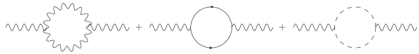
Figure 1: One loop corrections to the gluon propagator.

These coefficients are obtained from the 1 loop renormalised gauge couplings,

$$\beta_{i}=-\frac{\displaystyle{1}}{\displaystyle{4\pi}}\left[\frac{11}{3}~{}C_{2}(G_{i})-\frac{2}{3}\sum_{f}~{}T(R_{f})-\frac{1}{3}\sum_{S}~{}T(R_{s})\right]$$ (4)

with $C_{2}(G_{i})=N$ the eigenvalue of Casimir operator of the group $SU(N)$, and $T(R_{f})=T(R_{s})=1/2$ for fermions and scalars in the fundamental representation. The sums is extended over all fermions and scalars in the representations $R_{f}$ and $R_{s}$.

For the particle content of the SM, the $\beta$ coefficients read:

$$\beta_{3} = -\frac{\displaystyle{1}}{\displaystyle{4\pi}}\left[\frac{11}{3}\cdot 3-\frac{2}{3}\cdot 4~{}n_{g}\cdot\frac{1}{2}\right]=-\frac{\displaystyle{1}}{\displaystyle{4\pi}}\left[11-4\right],$$

$$\beta_{2} = -\frac{\displaystyle{1}}{\displaystyle{4\pi}}\left[\frac{11}{3}\cdot 2-\frac{2}{3}\cdot 4~{}n_{g}\cdot\frac{1}{2}-\frac{1}{3}\cdot n_{H}\cdot\frac{1}{2}\right]=-\frac{\displaystyle{1}}{\displaystyle{4\pi}}\left[\frac{22}{3}-4-\frac{1}{6}\right],$$

$$\beta_{1} = -\frac{\displaystyle{1}}{\displaystyle{4\pi}}\frac{3}{5}\left[-\frac{2}{3}\cdot\frac{10}{3}\cdot n_{g}-\frac{1}{3}\cdot n_{H}\cdot\frac{1}{2}\right]=-\frac{\displaystyle{1}}{\displaystyle{4\pi}}\left[-4-\frac{1}{10}\right],$$ (5)

with $n_{g}=3$ the number of generations and $n_{H}=1$ the number of Higgs doublets. Care must be taken in evaluating the $\beta_{1}$ coefficient of $U(1)$ hypercharge. Obviously its value depends on the normalisation one chooses for the hypercharge generator (indeed, hypercharge is related to the electric charge Q and the isospin $T_{3}$ by the relation $Q=T_{3}+aY$, with $a$ being the normalisation factor of the hypercharge generator Y). Asking for a unifying gauge symmetry group G embedding the SM to set in at the scale $M_{\mbox{\scriptsize GUT}}$ at which the SM couplings obtain a common value implies that all the SM generators are normalised in the same way. At this point the hypercharge normalisation is no longer arbitrary and the coefficient $\frac{3}{5}$ appearing in $\beta_{1}$ is readily explained (the interested reader is invited to explicitly derive this result , for instance considering one fermion family of the SM, computing $\mbox{Tr}(T)^{2}$ over such fermions and then imposing that $\mbox{Tr}(T)^{2}$=$\mbox{Tr}(Y)^{2}$).

Eq. (3) can be easily integrated and for a superlarge scale $M$ we obtain

$$\frac{\displaystyle{1}}{\displaystyle{\alpha_{i}(Q^{2})}}=\frac{\displaystyle{1}}{\displaystyle{\alpha_{i}(M^{2})}}+\beta_{i}~{}\log\frac{\displaystyle{M^{2}}}{\displaystyle{Q^{2}}}$$

$$\alpha_{i}(Q^{2})={\alpha_{i}(M^{2})\over\left(1+\beta_{i}\alpha_{i}(M^{2})\log\frac{\displaystyle{M^{2}}}{\displaystyle{Q^{2}}}\right)}$$ (6)

This result is very encouraging because we can see that both $\alpha_{3}$ and $\alpha_{2}$ decrease with increasing energies because $\beta_{3}$ and $\beta_{2}$ are negative. Moreover $\alpha_{3}$ decreases more rapidly because $|\beta_{3}|>|\beta_{2}|$. Finally $\beta_{1}$ is positive and hence $\alpha_{1}$ increases. Now we can ask whether starting from the measured values of the gauge couplings at low energies and using the $\beta_{i}$ parameters of the SM in Eq. (5) there is a scale, $M_{\mbox{\scriptsize GUT}}$, where the three couplings meet. To do this we have to solve the equations:

$$\frac{\displaystyle{1}}{\displaystyle{\alpha_{3}(\mu^{2})}} = \frac{\displaystyle{1}}{\displaystyle{\alpha_{\mbox{\scriptsize GUT}}}}+\beta_{3}~{}\log\frac{\displaystyle{M_{\mbox{\scriptsize GUT}}^{2}}}{\displaystyle{\mu^{2}}}$$

$$\frac{\displaystyle{1}}{\displaystyle{\alpha_{2}(\mu^{2})}} = \frac{\displaystyle{\sin^{2}\theta_{\rm W}(\mu^{2})}}{\displaystyle{\alpha_{\mbox{\scriptsize em}}(\mu^{2})}}=\frac{\displaystyle{1}}{\displaystyle{\alpha_{\mbox{\scriptsize GUT}}}}+\beta_{2}~{}\log\frac{\displaystyle{M_{\mbox{\scriptsize GUT}}^{2}}}{\displaystyle{\mu^{2}}}$$

$$\frac{\displaystyle{1}}{\displaystyle{\alpha_{1}(\mu^{2})}} = \frac{3}{5}~{}\frac{\displaystyle{\cos^{2}\theta_{\rm W}(\mu^{2})}}{\displaystyle{\alpha_{\mbox{\scriptsize em}}(\mu^{2})}}=\frac{\displaystyle{1}}{\displaystyle{\alpha_{\mbox{\scriptsize GUT}}}}+\beta_{1}~{}\log\frac{\displaystyle{M_{\mbox{\scriptsize GUT}}^{2}}}{\displaystyle{\mu^{2}}}$$ (7)

Now, we can use $\alpha_{3}$ and $\alpha_{\mbox{\scriptsize em}}$ to determine $M_{\mbox{\scriptsize GUT}}$ and then use the remaining equation to “predict” $\sin^{2}\theta_{\rm W}$:

$$\frac{\displaystyle{3}}{\displaystyle{5~{}\alpha_{\mbox{\scriptsize em}}(\mu^{2})}}-\frac{\displaystyle{8}}{\displaystyle{5~{}\alpha_{3}(\mu^{2})}}=\frac{\displaystyle{67}}{\displaystyle{20\pi}}~{}\log\frac{\displaystyle{M_{\mbox{\scriptsize GUT}}^{2}}}{\displaystyle{\mu^{2}}}$$

$$\sin^{2}\theta_{\rm W}(\mu^{2})=\frac{3}{8}\left[1-\frac{109}{36\pi}\alpha_{\mbox{\scriptsize em}}\log\frac{\displaystyle{M_{\mbox{\scriptsize GUT}}^{2}}}{\displaystyle{\mu^{2}}}\right].$$ (8)

The result is astonishing (we say this without any exaggeration!): starting from the measured values of $\alpha_{3}$ and $\alpha_{\mbox{\scriptsize em}}$ we find that all three gauge couplings would unify at a scale $M_{\mbox{\scriptsize GUT}}\simeq 2\times 10^{15}$ GeV if $\sin^{2}\theta_{\rm W}\simeq 0.21$. This is remarkably close to the experimental value of $\sin^{2}\theta_{\rm W}$ and this constitutes a major triumph of the grand unification idea and the strategy we adopted to implement it. Let us finally comment that in deriving these results we have used the so-called step approximation and one loop RGE equations. The step approximation consists in using the beta parameters of the SM (the three of them different) all the way from $M_{W}$ to $M_{\mbox{\scriptsize GUT}}$ where the beta parameter would change with a step function to a common beta parameter corresponding to $SU(5)$. In reality the $\beta$-function transitions from $\mu\ll M_{\mbox{\scriptsize GUT}}$ to $\mu\gg M_{\mbox{\scriptsize GUT}}$ are smooth ones that take into account the different threshold when new particles enter the RGE evolution. This effects can be included using mass dependent beta functions [29]. Similarly, we have only used one loop RGE equations although two loop RGE equations are also available. The inclusion of these additional refinements in our RGEs would not improve substantially the agreement with the experimental results.

2.1.1 The minimal SU(5) model of Georgi and Glashow

As has been discussed in the introduction, the SM gauge group has a rank four and the simple groups which contain complex representations of rank four are just $SU(3)\times SU(3)$ and $SU(5)$. Georgi and Glashow have chosen the $SU(5)$ where a single gauge coupling constant is manifestly incorporated. Further, the fermions of the Standard Model can be arranged in terms of the fundamental ${\bf\bar{5}}$ and the anti-symmetric ${\bf 10}$ representation of the SU(5) [30]. The appropriate particle assignments in these two representations are :

$${\bf\bar{5}}=\left(\matrix{d^{c}\cr d^{c}\cr d^{c}\cr\nu_{e}\cr e^{-}}\right)_{L} {\bf 10}=\left(\matrix{0&u^{c}&u^{c}&u&d\cr-u^{c}&0&u^{c}&u&d\cr-u^{c}&-u^{c}&0&u&d\cr-u&-u&-u&0&e^{c}\cr-d&-d&-d&-e^{c}&0}\right)_{L},$$ (9)

where ${\bf\bar{5}}=(\bar{3},1,-\frac{2}{3})+(1,2,-1)$ and ${\bf 10}=(3,2,\frac{1}{3})+(\bar{3},1,\frac{4}{3})+(1,1,-2)$ under $SU(3)\times SU(2)\times U(1)$ (here, we consider Y normalised as $Q=T_{3}+Y$, for simplicity). It is easy to check that this combination of the representations is anomaly free. The gauge theory of SU(5) contains 24 gauge bosons. They are decomposed in terms of the standard model gauge group SU(3) $\times$ SU(2) $\times$ U(1) as :

$${\bf 24=(8,1)+(1,3)+(1,1)+(3,2)+(\bar{3},2)}$$ (10)

The first component represents the gluon fields ($G$) mediating the colour, the second one corresponds to the Standard Model $SU(2)$ mediators ($W$) and the third component corresponds to the $U(1)$ mediator ($B$). The fourth and fifth components carry both colour as well as the $SU(2)$ indices and are called the $X$ and $Y$ gauge bosons. Schematically, the gauge bosons can be represented in terms of the $5\times 5$ matrix as:

$$V=\left(\begin{array}[]{ccccc}&&&X_{1}&Y_{1}\\ \lx@intercol\hfil\left[\frac{\displaystyle{(G-2B)}}{\displaystyle{\sqrt{30}}}\right]^{\alpha}_{\beta}\hfil\lx@intercol&X_{2}&Y_{2}\\ &&&X_{3}&Y_{3}\\ X_{1}&X_{2}&X_{3}&\frac{\displaystyle{W^{3}}}{\displaystyle{\sqrt{2}}}+\frac{\displaystyle{3B}}{\displaystyle{\sqrt{30}}}&W^{+}\\ Y_{1}&Y_{2}&Y_{3}&W^{-}&-\frac{\displaystyle{W^{3}}}{\displaystyle{\sqrt{2}}}+\frac{\displaystyle{3B}}{\displaystyle{\sqrt{30}}}\end{array}\right)$$ (11)

The particle spectrum is completed by the Higgs particles required to give masses to fermions as well as to break the GUT symmetry. To begin with, let us study the fermion masses in the prototype $SU(5)$. Given that fermions are in ${\bf\overline{5}}$ and ${\bf 10}$ representations, after some simple algebra we conclude that the scalars that can form Yukawa couplings are

$${\bf 10\times 10} = {\bf\overline{5}+\overline{45}+50}$$ (12)

$${\bf 10\times\overline{5}} = {\bf 5+45}$$ (13)

From the above, we see that we need at least two Higgs representations transforming as the fundamental (${\bf 5}_{H}$) and the anti-fundamental (${\bf\overline{5}}_{H}$) to reproduce the fermion Yukawa couplings. The corresponding Yukawa terms read: :

$$\mathcal{L}^{\rm yuk}_{SU(5)}=h^{u}_{ij}{\bf 10_{i}10_{j}\overline{5}}_{H}+h^{d}_{ij}{\bf 10_{i}\overline{5}_{j}5}_{H}$$ (14)

Though the Yukawa couplings written above are quite simple, they do not stand the test of phenomenological constraints, as we will see later. A Higgs in the adjoint representation can be used to break $SU(5)$ to the diagonal subgroup of the Standard Model. Denoting the adjoint as $\Phi=\sum_{i=1}^{24}\lambda_{i}/\sqrt{2}\phi_{i}$ , where $\lambda_{i}$ are generators of the SU(5), the most general renormalisable scalar potential is

$$V(\Phi)=-{1\over 2}m_{1}^{2}\mbox{Tr}(\Phi^{2})+{1\over 4}a(\mbox{Tr}(\Phi^{2}))^{2}+{1\over 2}b\mbox{Tr}(\Phi^{4})+{1\over 3}c\mbox{Tr}(\Phi^{3}).$$ (15)

However, to simplify the potential, we impose a discrete symmetry ($\Phi~{}\leftrightarrow~{}-\Phi$) which sets $c$ to zero. The remaining potential has the following minimum when $b>0$ and $a>-7/15~{}b$:

$$<0|\Phi|0>=\left(\begin{array}[]{ccccc}v&0&0&0&0\\ 0&v&0&0&0\\ 0&0&v&0&0\\ 0&0&0&-3/2v&0\\ 0&0&0&0&-3/2v\end{array}\right),$$ (16)

with $v$ determined by

$$m_{1}^{2}={15\over 2}av^{2}+{7\over 2}bv^{2}$$ (17)

This completes the proto-GUT model containing all the required features : gauge coupling unification, representations accomodating all SM fermions, yukawa couplings for fermion masses, gauge symmetry breaking down to SM gauge group. However as usual in real life, things are a bit more complicated as we will see now.

2.1.2 Distinctive Features of GUTs and Problems in building a realistic Model

(i) Fermion Masses
In the previous section, we have seen that in the typical prototype SU(5) model, the fermions attain their masses through a $5_{H}$ and $\bar{5}_{H}$ of Higgses. A simple consequence of this approach is that there is an equality of $Y_{d}^{T}~{}=~{}Y_{e}$ at the GUT scale; which would mean equal charged lepton and down quark masses at the $M_{\rm GUT}$ scale. Schematically, these are given as:

$$m_{e}(M_{\mbox{\scriptsize GUT}}) = m_{d}(M_{\mbox{\scriptsize GUT}})$$ (18)

$$m_{\mu}(M_{\mbox{\scriptsize GUT}}) = m_{s}(M_{\mbox{\scriptsize GUT}})$$ (19)

$$m_{\tau}(M_{\mbox{\scriptsize GUT}}) = m_{b}(M_{\mbox{\scriptsize GUT}}).$$ (20)

We would have to verify these prediction by running the Yukawa couplings from the SM to the GUT scale. Let us have a more closer look at these RGEs. For the bottom mass and the $\tau$ Yukawa these are given by [31, 32] :

$${d\log Y_{b}(\mu)\over d\log\mu} = -3~{}C_{3}^{b}\frac{\displaystyle{\alpha_{3}(\mu)}}{\displaystyle{4\pi}}-3~{}C_{2}^{b}\frac{\displaystyle{\alpha_{2}(\mu)}}{\displaystyle{4\pi}}-3~{}C_{1}^{b}\frac{\displaystyle{\alpha_{1}(\mu)}}{\displaystyle{4\pi}}$$ (21)

$${d\log Y_{\tau}(\mu)\over d\log\mu} = -3~{}C_{3}^{\tau}\frac{\displaystyle{\alpha_{3}(\mu)}}{\displaystyle{4\pi}}-3~{}C_{2}^{\tau}\frac{\displaystyle{\alpha_{2}(\mu)}}{\displaystyle{4\pi}}-3~{}C_{1}^{\tau}\frac{\displaystyle{\alpha_{1}(\mu)}}{\displaystyle{4\pi}}$$ (22)

with $C_{3}^{b}=\frac{4}{3}$, $C_{2}^{b}=\frac{3}{4}$, $C_{1}^{b}=-\frac{1}{30}$, $C_{3}^{\tau}=0$, $C_{2}^{\tau}=\frac{3}{4}$, $C_{1}^{\tau}=-\frac{3}{10}$. Knowing the scale dependence of the gauge couplings, Eq. (2.1), we can integrate this equation, neglecting the effects of other Yukawa except the top Yukawa in the RHS of the above equations. Taking the masses to be equal at $M_{\mbox{\scriptsize GUT}}$, we obtain

$${m_{b}(M_{Z})\over m_{\tau}(M_{Z})}\approx E_{t}^{-1/2}\left[{\alpha_{3}(M_{Z})\over\alpha_{3}(M_{\mbox{\scriptsize GUT}})}\right]^{-3C_{3}\over 4\pi\beta_{3}}\approx E_{t}^{-1/2}\left[{\alpha_{3}(M_{Z})\over\alpha_{3}(M_{\mbox{\scriptsize GUT}})}\right]^{4\over 7},$$ (23)

where $E_{t}={\rm Exp}[{1\over 2\pi}\int_{M_{Z}}^{M_{\rm GUT}}Y_{t}(t)dt]$. Taking these masses at the weak scale, we obtain a rough relation

$${m_{b}(M_{W})\over m_{\tau}(M_{W})}\approx 3,$$ (24)

which is quite in agreement with the experimental values. This can be considered as one of the major predictions of the $SU(5)$ grand unification. However, there is a caveat. If we extend similar analysis to the first two generations we end-up with relations :

$${m_{\mu}\over m_{e}}={m_{s}\over m_{d}},$$ (25)

which don’t hold water at weak scale. The question remains how can one modify the bad relations of the first two generations while keeping the good relation of the third generation intact. Georgi and Jarlskog solved this puzzle [33] with a simple trick using an additional Higgs representation. As we have seen in Eq. (13), the ${\bf 10}$ and ${\bf\bar{5}}$ can couple to a ${\bf 45}$ in addition to the ${\bf 5}$ representation. The ${\bf 45}$ is a completely anti-symmetric representation and a texture can be chosen such that the bad relations can be modified keeping the good relation intact.

(ii) Doublet-Triplet Splitting
We have seen that in minimal $SU(5)$ we need at least two Higgs representations transforming as ${\bf 5_{H}}$ and ${\bf\bar{5}_{H}}$ to accommodate the fermion Yukawa couplings. The ${\bf 5}$ representation of $SU(5)$ contains a $({\bf 3},{\bf 1})$ and $({\bf 1},{\bf 2})$ under $(SU(3)_{C},SU(2)_{\rm L})$. So, the ${\bf 5_{H}}$ and ${\bf\bar{5}_{H}}$ representations contain the required Higgs doublets that breaks the electroweak symmetry at low energies, but they contain also colour triplets, extremely dangerous, as we will see later, because they mediate a fast proton decay if their mass is much lower than the GUT scale. The doublet-triplet splitting problem is then the question of how one can enforce the mass of the Higgs doublet to remain at the electroweak scale, while the Higgs triplet mass should jump to $M_{\mbox{\scriptsize GUT}}$ [34].

The $SU(5)$ symmetry is broken by the VEV of the Higgs $\Phi$ sitting in the adjoint representation, as we saw in Eq. (15). At the electroweak scale we need a second breaking step, $SU(3)_{C}\times SU(2)_{\rm L}\times U(1)_{Y}\to SU(3)_{C}\times U(1)_{\mbox{\scriptsize em}}$, which is obtained by the potential

$$V(H)=-\frac{\displaystyle{\mu^{2}}}{\displaystyle{2}}{\bf 5_{H}}^{\dagger}{\bf 5_{H}}+\frac{\displaystyle{\lambda}}{\displaystyle{4}}\left({\bf 5_{H}}^{\dagger}{\bf 5_{H}}\right)^{2},$$ (26)

with a VEV

$$\langle{\bf 5_{H}}\rangle=\left(\begin{array}[]{c}0\\ 0\\ 0\\ 0\\ \frac{v_{0}}{\sqrt{2}}\end{array}\right),\qquad v_{0}^{2}=\frac{\displaystyle{2\mu^{2}}}{\displaystyle{\lambda}}.$$ (27)

However, the potential $V=V(\Phi)+V(H)$ does not give rise to a viable model. Clearly both the Higgs doublet and triplet fields remain with masses at the $M_{W}$ scale which is catastrophic for proton decay.

This problem can find a solution if we consider also the following $\Phi$–${\bf 5_{H}}$ cross terms which are allowed by $SU(5)$

$$V(\Phi,H)=\alpha{\bf 5_{H}}^{\dagger}{\bf 5_{H}}\mbox{Tr}(\Phi^{2})+\beta{\bf 5_{H}}^{\dagger}\Phi^{2}{\bf 5_{H}}.$$ (28)

Notice that even if one does not introduce the above mixed term at the tree level, one expects it to arise at higher order given that the underlying $SU(5)$ symmetry does not prevent its appearance.

Let’s turn to the minimisation of the full potential $V=V(\Phi)+V(H)+V(\Phi,H)$. Now that $\Phi$ and ${\bf 5_{H}}$ are coupled, $\langle\Phi\rangle$ may also break $SU(2)_{\rm L}$ whilst $SU(3)_{C}$ must be rigorously unbroken. Therefore, we look for solutions with $\langle\Phi\rangle={\rm Diag.}\left(v,v,v,\left(-\frac{3}{2}-\frac{\varepsilon}{2}\right)v,\left(-\frac{3}{2}-\frac{\varepsilon}{2}\right)v\right)$. In the absence of $\Phi$–${\bf 5_{H}}$ mixing, i.e. $\alpha=\beta=0$, $\varepsilon$ must vanish. The solution with this properties has

$$\varepsilon=\frac{\displaystyle{3}}{\displaystyle{20}}~{}\frac{\displaystyle{\beta v_{0}^{2}}}{\displaystyle{bv^{2}}}+O\left(\frac{\displaystyle{v_{0}^{4}}}{\displaystyle{v^{4}}}\right).$$ (29)

As $v\sim O\left(M_{\mbox{\scriptsize GUT}}\right)$ and $v_{0}\sim O\left(M_{W}\right)$, we have that the breaking of $SU(2)$ due to $\langle\Phi\rangle$ is much smaller than that due to $\langle H\rangle$. Now, the expressions for $m_{1}^{2}$ (corresponding to Eq. (17)) and $\mu_{5}^{2}$ (corresponding to Eq. (27)) are more complicated

$$m_{1}^{2}={15\over 2}av^{2}+{7\over 2}{15}bv^{2}++\alpha v_{0}^{2}+{9\over 30}\beta v_{0}^{2}$$ (30)

and

$$\mu^{2}={1\over 2}\lambda v_{0}^{2}+{15}\alpha v^{2}+{9\over 2}\beta v^{2}-3\epsilon\beta v^{2}.$$ (31)

We can see that Eq. (30) shows only a very small modification from Eq. (17) being $v_{0}\ll v$. What is very worrying is the result of Eq. (31). Since the parameter in the Lagrangian $\mu\sim O(M_{W})$, i.e. $\mu\ll v$, the natural thing to happen would be that $v_{0}$ takes a value order $v$ to reduce the right-hand side of this equation (remember that in this equation $v$ and $v_{0}$ are our unknowns). In other words, without putting any particular constraint on $\alpha$ and $\beta$, we would expect $v_{0}\sim O(v)$. However, this would completely spoil the hierarchy between $M_{W}$ and $M_{\mbox{\scriptsize GUT}}$. If we want to avoid such a disaster, we have to fine-tune $\alpha$ and $\beta$ to one part in $\left({v^{2}\over v_{0}^{2}}\right)\sim 10^{24}$!!! Even more, such an adjustment must be repeated at every order in perturbation theory, since radiative correction will displace $\alpha$ and $\beta$ for more than one part in $10^{24}$. This is our first glimpse in the so-called hierarchy problem.

(iii). Nucleon Decay
As we saw in the previous section, perhaps the most prominent feature of GUT theories is the non-conservation of baryon (and lepton) number. In the minimal $SU(5)$ model this is due to the tree-level exchange of $X$ and $Y$ gauge bosons in the adjoint of $SU(5)$ with $({\bf 3},{\bf 2})$ quantum numbers under $SU(3)\times SU(2)_{\rm L}$. The couplings of these gauge bosons to fermions are

$${\cal L}_{X}=\sqrt{\frac{1}{2}}gX^{a}_{\mu\alpha}\left[\epsilon^{\alpha\beta\gamma}~{}\overline{u}^{c}_{\gamma}\gamma^{\mu}q_{\beta a}+\epsilon^{ab}\left(\overline{q}_{\alpha b}\gamma^{\mu}e^{+}-\overline{l}_{b}\gamma^{\mu}d^{c}_{\alpha}\right)\right],$$ (32)

where $\epsilon_{\alpha\beta\gamma}$ and $\epsilon_{ab}$ are the totally antisymmetric tensors, $(\alpha,\beta,\gamma)$ are $SU(3)$ and $a,b$ are $SU(2)_{\rm L}$ indices. Thus the $SU(2)_{\rm L}$ doublets are

$$X_{\alpha a}=\left(X_{\alpha},Y_{\alpha}\right),\quad q_{\alpha a}=\left(u_{\alpha},u_{\alpha}\right),\quad l_{a}=\left(\nu_{e},e\right).$$ (33)

We can see in Eq. (32) that the $(X,Y)$ bosons have two couplings to fermions with different baryon numbers. They have a leptoquark coupling with $B_{1}=-1/3$ and a diquark couplings with $B_{2}=2/3$. Therefore, through the coupling of an $X$ boson we can change a $B=-1/3$ channel into a $B=2/3$ channel and a $\Delta B=1$ process occurs at tree level as shown in Figure 2.

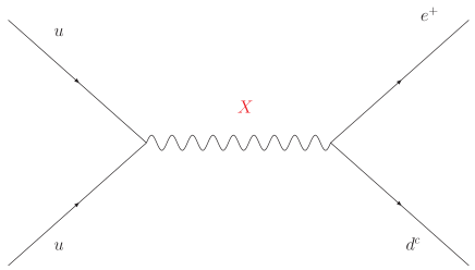
Figure 2: Baryon number violating couplings of the $X$ boson.

If the mass of the $X$ boson, $M_{X}$ is large compared to the other masses, we can obtain the effective four-fermion interactions [35, 36, 37, 38]

$${\cal L}_{\Delta B=1}^{\rm eff}=\frac{\displaystyle{g^{2}}}{\displaystyle{2M_{X}^{2}}}~{}\epsilon^{\alpha\beta\gamma}\epsilon^{ab}\left(\overline{u}^{c}_{\gamma}\gamma^{\mu}q_{\beta a}\right)\left(\overline{d}^{c}_{\alpha}\gamma_{\mu}l_{b}+\overline{e}^{+}\gamma_{\mu}q_{\alpha b}\right).$$ (34)

From this effective Lagrangian we can see that although baryon number is violated, $(B-L)$ is still conserved, thus the decay $p\to e^{+}\pi^{0}$ is allowed but a decay $n\to e^{-}\pi^{+}$ is forbidden. From this effective Lagrangian we can obtain the proton decay rate and we have $\Gamma_{p}\sim 10^{-3}m_{p}^{5}/M_{X}^{4}$ and therefore from the present bound on the proton lifetime $\tau_{p}\geq 10^{33}$ yrs, we have that $M_{X}\geq 4\times 10^{15}$ GeV. From this simple dimensional estimate of the proton decay lifetime, we can already see that the minimal non-supersymmetric $SU(5)$ can easily get into trouble because of matter stability. Indeed, performing an accurate analysis of proton decay, even taking into account the relevant theoretical uncertainty factors, like the evaluation of the hadronic matrix element, one can safely conclude that the minimal grand unified extension of the SM is ruled out because of the exceedingly high matter instability. Analogously, the high precision achieved on electroweak observables (in particular thanks to LEP physics) allows us to further exclude the minimal SU(5) model: indeed, the low-energy quantity one can predict solving the RGE’s for the gauge coupling evolution (be it the electroweak angle $\theta_{W}$, or the strong coupling $\alpha_{s}$) exhibits a large discrepancy with respect to its measured value. The precise $SU(5)$ prediction for $\sin^{2}\theta_{W}$ is [39]:

$$\sin^{2}\theta_{W}(M_{W})=0.214^{+0.004}_{-0.003},$$ (35)

while the experimental value obtained from LEP data is:

$$\sin^{2}\theta_{W}(M_{W})=0.23108\pm 0.00005,$$ (36)

and both values only agree at 5 standard deviations.

The fate of the minimal $SU(5)$ should not induce the reader to conclude “tout-court” that non-supersymmetric grand unification is killed by proton decay and $sin^{2}\theta_{W}$. Once one abandons the minimality criterion, for instance enlarging the Higgs spectrum or changing the grand unified gauge group, it is possible to rescue some GUT models. The price to pay for it is that we lose the simplicity and predictivity of minimal SU(5) ending up in more and more complicated grand unified realisations.

2.2 Supersymmetric grand unification

2.2.1 The hierarchy problem and supersymmetry

The Standard Model as a $SU(3)\otimes SU(2)\otimes U(1)$ gauge theory with three generations of quarks and leptons and a Higgs doublet provides an accurate description of all known experimental results. However, as we have discussed, the SM cannot be the final theory, and instead we consider the SM as a low energy effective theory of some more fundamental theory at higher energies. Typically we have a Grand Unification (GUT) Scale around $10^{16}$ GeV where the strong and electroweak interactions unify in a simple group like $SU(5)$ or $SO(10)$ [24, 25] and the Plank scale of $10^{19}$ GeV where these gauge interactions unify with gravity. The presence of such different scales in our theory gives rise to the so–called hierarchy problem (see a nice discussion in [40]). This problem refers to the difficulty to stabilise the large gap between the electroweak scale and the GUT or Plank scales under radiative corrections. Such difficulty arises from a general property of the scalar fields in a gauge theory, namely their tendency of scalar to get their masses in the neighbourhood of the largest available energy scale in the theory. In the previous section, when dealing with the scalar potential of the minimal $SU(5)$ model, we have directly witnessed the existence of such problem. From such a particular example, let us move to more general considerations about what distinguishes the behaviour of scalar fields from that of fermion and vector fields in gauge theories.

To understand this problem let us compare the one loop corrections to the electron mass and the Higgs mass. These one loop corrections are given by the diagrams in Fig. 3.

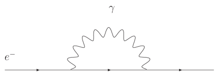
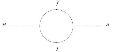
Figure 3: One loop correction to fermion and scalar masses

The self-energy contribution to the electron mass can be calculated from this diagram to be,

$$\delta m_{e}=2\frac{\displaystyle{\alpha_{em}}}{\displaystyle{\pi}}m_{e}\log\frac{\displaystyle{\Lambda}}{\displaystyle{m_{e}}}$$ (37)

and it is logarithmically divergent. Here we have regulated the integral with an ultraviolet cutoff $\Lambda$. However, it is important to notice that this correction is proportional to the electron mass itself. This can be understood in terms of symmetry. In the limit where $m_{e}\to 0$, our theory acquires a new chiral symmetry where right-handed and left-handed electrons are decoupled. Were such a symmetry exact, the one loop corrections to the mass would have to vanish. This chiral symmetry is only broken by the electron mass itself and therefore any loop correction breaking this symmetry must be proportional to $m_{e}$, the only source of chiral symmetry breaking in the theory. This has important implications. If we replace the cutoff $\Lambda$ by the largest possible scale, the Planck mass we get,

$$\delta m_{e}=2\frac{\displaystyle{\alpha_{em}}}{\displaystyle{\pi}}m_{e}\log\frac{\displaystyle{M_{Plank}}}{\displaystyle{m_{e}}}\simeq 0.24~{}m_{e},$$ (38)

which is only a small correction to the electron mass.

Analogously, for the gauge vector bosons there is the gauge symmetry itself which constitutes the “natural barrier” preventing their masses to become arbitrarily large. Indeed, if a vector boson V is associated to the generator of a certain symmetry G, as long as G is unbroken the vector V has to remain massless. Its mass will be of the order of the scale at which the symmetry G is (spontaneously) broken. Hence, once again, we have a symmetry protecting the mass of vector bosons.

On the other hand, the situation is very different in the case of the Higgs boson,

$$\delta m_{H}^{2}(f)=-2N_{f}\frac{\displaystyle{|\lambda_{f}|^{2}}}{\displaystyle{16\pi^{2}}}[\Lambda^{2}-2m_{f}^{2}\ln\frac{\displaystyle{\Lambda}}{\displaystyle{m_{f}}}+\dots].$$ (39)

But, in this case, the one loop contribution is quadratically divergent !!. This is due to the fact that no symmetry protects the scalar mass and in the limit $m_{H}^{2}\to 0$ the symmetry of our model is not increased. The combination $HH^{\dagger}$ is always neutral under any symmetry independently of the charges of the field $H$. So, the scalar mass should naturally be of the order of the largest scale of the theory, as either at tree level or at loop level this scale feeds into the scalar mass.

So, if now we repeat the exercise we made with the electron mass and replace the cutoff by the Plank mass, we obtain $\delta m_{H}^{2}\ \simeq\ 10^{30}\mbox{ GeV}^{2}$. In fact we could cancel these large correction with a bare mass of the same order and opposite sign. However, these two contributions should cancel with a precision of one part in $10^{26}$ and even then we should worry about the two loop contribution and so on. This is the so-called hierarchy problem and Supersymmetry constitutes so far the most interesting answer to it (later on, we’ll briefly comment on the existence of other approaches tackling the hierarchy problem, although, in our view, not as effectively as low-energy supersymmetry does).

As we have seen in the previous section, Supersymmetry associates a fermion with every scalar in the theory with, in principle, identical masses and gauge quantum numbers. Therefore, in a Supersymmetric theory we would have a new contribution to the Higgs mass at one loop.

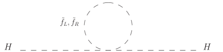
Figure 4: Additional Supersymmetric contribution to the scalar mass.

Now this graph gives a contribution to the Higgs mass as,

$$\delta m_{H}^{2}(\tilde{f})=-2N_{\tilde{f}}\frac{\displaystyle{\lambda_{\tilde{f}}}}{\displaystyle{16\pi^{2}}}[\Lambda^{2}-\ 2m_{\tilde{f}}^{2}\ln\frac{\displaystyle{\Lambda}}{\displaystyle{m_{\tilde{f}}}}\ +\dots]$$ (40)

If we compare Eqs. (39) and (40) we see that with $N_{f}=N_{\tilde{f}}$, $|\lambda_{f}|^{2}=-\lambda_{\tilde{f}}$ and $m_{f}=m_{\tilde{f}}$ we obtain a total correction $\delta m_{H}^{2}(f)+\delta m_{H}^{2}(\tilde{f})=0$ !!. This means we need a symmetry that associates a bosonic partner to every fermion with equal mass and related couplings and this symmetry is Supersymmetry.

Still, we have not found scalars exactly degenerate with the SM fermions in our experiments. In fact, it would have been very easy to find a scalar partner of the electron if it existed. Thus, Supersymmetry can not be an exact symmetry of nature, it must be broken. Fortunately, we can break Supersymmetry while at the same time preserving to an acceptable extent the Supersymmetric solution of the hierarchy problem. To do that, we want to ensure the cancellation of quadratic divergences and comparing Eq. (39) and Eq. (40) we can see that we must still require equal number of scalar and fermionic degrees of freedom, $N_{f}=N_{\tilde{f}}$, and supersymmetric dimensionless couplings $|\lambda_{f}|^{2}=-\lambda_{\tilde{f}}$. Supersymmetry can be broken only in couplings with positive mass dimension, as for instance the masses. This is called soft breaking [41]. Now if we take $m_{\tilde{f}}^{2}=m_{f}^{2}+\delta^{2}$ we obtain a correction to the Higgs mass,

$$\delta m_{H}^{2}(f)+\delta m_{H}^{2}(\tilde{f})\simeq 2N_{f}\frac{\displaystyle{|\lambda_{f}|^{2}}}{\displaystyle{16\pi^{2}}}\ \delta^{2}\ \ln\frac{\displaystyle{\Lambda}}{\displaystyle{m_{\tilde{f}}}}+\dots$$ (41)

and this is only logarithmically divergent and proportional to the mass difference between the fermion and its scalar partner. Still we must require this correction to be smaller than the Higgs mass itself (around the electroweak scale) implies that this mass difference, $\delta$, can not be too large, in fact $\delta\raise 1.29167pt\hbox{$\;<$\kern-7.5pt\raise-4.73611pt\hbox{$\sim\;$}}1\mbox{ TeV}$. If Supersymmetry is the solution to the hierarchy problem it must be softly broken and the SUSY partners must be roughly below 1 TeV. The rich SUSY phenomenology is thoroughly discussed in Marcela Carena and Carlos Wagner’s lectures at this School [42].

2.3 Gauge coupling Unification in SUSY $SU(5)$

The supersymmetric $SU(5)$ can be build analogously to the non-supersymmetric $SU(5)$ with the ordinary fields replaced by superfields containing the SM field and its superpartner. What is relevant for our discussion on grand unification at present is the effect of the presence of new SUSY particles at 1 TeV in the evolution of the gauge couplings. We saw in the previous section that the RGE equations in the SM predict that the gauge couplings get very close at a large scale $\simeq 2\times 10^{15}$ GeV. Nevertheless this unification was not perfect and, using the precise determination of the gauge couplings at LEP we see that the SM couplings do not unify at seven standard deviations. If we have new SUSY particles around 1 TeV, these RGE equations are modified. Using Eq. (4), it is straightforward to obtain the new $\beta_{i}$ parameters in the MSSM. We have to take into account that for every gauge boson we have to add a fermion, called gaugino, both in the adjoint representation. Therefore from gauge bosons and gauginos we have

$$\beta_{i}(V)=-\frac{\displaystyle{1}}{\displaystyle{4\pi}}\left[\frac{11}{3}~{}C_{2}(G_{i})-\frac{2}{3}C_{2}(G_{i})\right]=-\frac{\displaystyle{1}}{\displaystyle{4\pi}}~{}3~{}C_{2}(G_{i}).$$ (42)

While for every fermion we have a corresponding scalar partner in the same representation. Thus we have

$$\beta_{i}(F)=-\frac{\displaystyle{1}}{\displaystyle{4\pi}}\sum_{F}\left[-\frac{2}{3}~{}T(R_{F})-\frac{1}{3}~{}T(R_{F})\right]=\frac{\displaystyle{1}}{\displaystyle{4\pi}}~{}\sum_{F}T(R_{F}),$$ (43)

summed over all the chiral supermultiplet (fermion plus scalar) representations. Therefore the total $\beta_{i}$ coefficient in a supersymmetric model is

$$\beta_{i}=-\frac{\displaystyle{1}}{\displaystyle{4\pi}}\left[3~{}C_{2}(G_{i})-\sum_{F}T(R_{F})\right].$$ (44)

And for the MSSM

$$\beta_{3} = -\frac{\displaystyle{1}}{\displaystyle{4\pi}}\left[9-2~{}n_{g}\right]=-\frac{\displaystyle{3}}{\displaystyle{4\pi}},$$

$$\beta_{2} = -\frac{\displaystyle{1}}{\displaystyle{4\pi}}\left[6-2~{}n_{g}-\frac{1}{2}~{}n_{H}\right]=+\frac{\displaystyle{1}}{\displaystyle{4\pi}},$$

$$\beta_{1} = -\frac{\displaystyle{1}}{\displaystyle{4\pi}}\left[-\frac{10}{3}~{}n_{g}-\frac{1}{2}~{}n_{H}\right]=+\frac{\displaystyle{11}}{\displaystyle{4\pi}}.$$ (45)

From the comparison of Eq. (5) and Eq. (45) we see that the evolution of the gauge couplings is significantly modified. We can easily calculate the grand unification scale and the “predicted” value of $\sin^{2}\theta_{\rm W}$ as done in Eqs. (7) and (2.1) and we obtain

$$\qquad M_{\mbox{\scriptsize GUT}}^{\rm MSSM}=1.5\times 10^{16}\mbox{GeV}, \qquad\sin^{2}\theta_{\rm W}(M_{Z})=0.234,$$ (46)

which is remarkably close to the experimental vale $\sin^{2}\theta_{\rm W}^{\rm exp}(M_{Z})=0.23149\pm 0.00017$. And we obtain easily the grand unified coupling constant

$${5\over 3}\alpha_{1}(M_{\mbox{\scriptsize GUT}})=\alpha_{2}(M_{\mbox{\scriptsize GUT}})=\alpha_{3}(M_{\mbox{\scriptsize GUT}})\approx{1\over 24}$$ (47)

In fact, the actual analysis, including two loop RGEs and threshold effects predicts $\alpha_{3}(M_{Z})=0.129$ which is slightly higher than the observed value (such discrepancy could be justified by the presence of threshold effects when approaching the GUT scale in the running). The couplings meet at the value $M_{X}=2\times 10^{16}$ GeV [43, 44, 45]. The “exact” unification of the gauge couplings within the MSSM may or may not be an accident. But it provides enough reasons to consider supersymmetric standard models seriously as it links supersymmetry and grand unification in an inseparable manner [46]. Let us know see how the other GUT features and problems which we have encountered earlier in non-supersymmetric theories fare in the supersymmetric GUTs.

2.3.1 SUSY GUT predictions and problems

(i ) Doublet-Triplet Splitting
As we saw in the non-supersymmetric case, a very accurate fine-tuning in the parameters of the scalar potential was required to reproduce the hierarchy between the electroweak and the GUT scale. In a supersymmetric grand unified theory the problem is very similar. The relevant terms in the superpotential are,

$$W=\alpha{\bf\overline{5}_{H}}\Phi^{2}{\bf 5_{H}}+\mu{\bf\overline{5}_{H}}{\bf 5_{H}}.$$ (48)

The breaking of $SU(5)$ in the $SU(3)\times SU(2)\times U(1)$ direction via

$$\langle\Phi\rangle={2~{}m^{\prime}\over 3~{}\alpha}~{}{\rm Diag.}~{}\left(1,1,1,-\frac{3}{2},-\frac{3}{2}\right),$$ (49)

leads to

$$W={\bf\overline{3}_{H}}{\bf 3_{H}}\left(\mu+{2\over 3}m^{\prime}\right)+{\bf\overline{2}_{H}}{\bf 2_{H}}\left(\mu-m^{\prime}\right).$$ (50)

Choosing $\mu=m^{\prime}$ (both them $\sim O(M_{\mbox{\scriptsize GUT}})$) renders the Higgs doublets massless. However, although due to supersymmetry this equality is stable under radiative corrections, this extremely accurate adjustment is extremely unnatural.

There are several mechanisms in supersymmetric theories to render doublet-triplet splitting natural. Here we will briefly discus the “missing partner mechanism” [47]. From Eq. (50) we see that if the direct mass term for the Higgses, $\mu$, was absent the doublets would obtain super-heavy masses from the vacuum expectation value of the adjoint Higgs $\Phi$. The strategy we will use to solve the doublet-triplet splitting problem is to introduce representations that contain Higgs triplets but no doublets. We can choose the ${\bf 50}$ that is decomposed under $SU(3)\times SU(2)$ as:

$${\bf 50=(8,2)+(6,3)+(\bar{6},1)+(3,2)+(\bar{3},1)+(1,1)}$$ (51)

We need both the ${\bf 50}$ and ${\bf\bar{5}0}$ to get an anomaly-free model. In order to write mixing terms between ${\bf 5}$, ${\bf\bar{5}}$ and ${\bf 50}$, ${\bf\bar{5}0}$ we need a field $\Sigma$ in the ${\bf 75}$ instead of the ${\bf 24}$ to break $SU(5)$. The relevant part of superpotential is then

$$W={M\over 2}\mbox{Tr}(\Sigma^{2})+{a\over 3}~{}\mbox{Tr}(\Sigma^{3})+b~{}{\bf 50}~{}{\Sigma}~{}{\bf 5_{H}}+c~{}{\bf\bar{5}0}~{}{\Sigma}~{}{\bf\bar{5}_{H}}+\tilde{M}~{}{\bf\bar{5}0}~{}{\bf 50},$$ (52)

where no mass term ${\bf\bar{5}_{H}}~{}{\bf 5_{H}}$ is present. ${\Sigma}$ gets a VEV, $\langle{\Sigma}\rangle\sim\frac{M}{a}$, breaking $SU(5)$ to $SU(3)\times SU(2)\times U(1)$. The resulting $SU(3)\times SU(2)\times U(1)$ superpotential is,

$$W={\bf 50_{3}}~{}{\frac{M~{}b}{a}}~{}{H_{3}}+{\bf\bar{5}0_{3}}~{}{\frac{M~{}c}{a}}~{}{\bar{H}_{3}}+\tilde{M}~{}{\bf\bar{5}0_{3}}~{}{\bf 50_{3}},$$ (53)

with $H_{3}$ and ${\bf 50_{3}}$ the Higgs triplets in the ${\bf 5_{H}}$ and ${\bf 50}$ representations respectively. Therefore the Higgs triplets get a mass of the order of $M\sim\tilde{M}\sim M_{\mbox{\scriptsize GUT}}$ and the Higgs doublets remain massless because there is no mass term for the doublets. In this way we solve the doublet-triplet splitting problem without unnatural fine-tuning of the parameters.

(ii) Proton Decay
In the non-supersymmetric $SU(5)$ proton decay arises from four fermion operators, hence from operators of canonical dimension 6. In addition to such dim=6 operators, in the supersymmetric case we encounter also dim=5 and even dim=4 operators leading to proton decay.

Dimension 4 operators are not suppressed by any power of the GUT scale. In fact, these terms are gauge invariant and in principle are allowed to appear in the superpotential,

$$W_{\Delta L=1}=\lambda^{ijk}L_{i}L_{j}e^{c}_{Rk}+\lambda^{\prime\;ijk}L_{i}Q_{j}d^{c}_{Rk}+\epsilon^{i}L_{i}H_{2}$$

$$W_{\Delta B=1}=\lambda^{\prime\prime\;ijk}\;u^{c}_{Ri}d^{c}_{Rj}d^{c}_{Rk}~{}~{}~{}~{}~{}~{}~{}~{}~{}~{}~{}~{}~{}~{}~{}$$ (54)

However, these terms violate baryon or lepton number by 1 unit. So, these terms are very dangerous. Indeed, if $\lambda^{\prime}$ and $\lambda^{\prime\prime}$ are simultaneously present, a very fast proton decay arises through the diagram in Figure 5.

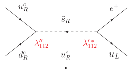
Figure 5: Proton decay through R-parity violating couplings.

Clearly, the major difference is that in the non-SUSY case the mediation of proton decay occurs through the exchange of super-heavy (vector or scalar) bosons whose masses are at the GUT scale. On the contrary, in Figure 5 the mediator is a SUSY particle and, hence, at least if we insist in invoking low-energy SUSY to tackle the hierarchy problem, its mass is at the electroweak scale instead of being at $M_{\mbox{\scriptsize GUT}}$! From the bounds to the decay $p^{+}\to e^{+}\pi^{0}$ we obtain $\lambda^{\prime\;*}_{112}\cdot\lambda^{\prime\prime}_{112}\leq 2\times 10^{-27}$. Clearly this product is too small and it is more natural to consider it as exactly zero. Other couplings from Eq. (54) are not so stringently bounded but in general all of them must be very small from phenomenological considerations (in particular, from FCNC constraints).

One possibility is to introduce a new discrete symmetry, called R-parity to forbid these terms. R-parity is defined as $R_{P}=(-1)^{3B+L+2S}$ such that the SM particles and Higgs bosons have $R_{P}=+1$ and all superpartners have $R_{P}=-1$. In the MSSM $R_{P}$ is conserved and this has some interesting consequences.

• $W_{\Delta L=1}$ and $W_{\Delta B=1}$ are absent in the MSSM.

• The Lightest Supersymmetric Particle (LSP) is completely stable and it provides a (cold) dark matter candidate.

• Any sparticle produced in laboratory experiments decays into a final state with an odd number of LSP.

• In colliders, Supersymmetric particles can only be produced (or destroyed) in pairs.

A second contribution to proton decay, already present in non-SUSY GUTs, comes from dimension 6 operators. The discussion is analogous to the analysis in non-SUSY GUTS. Here we will only recall that a generic four-fermion operator of the form $1/\Lambda^{2}~{}q~{}q~{}q~{}l$ results in a proton decay rate of the order $\Gamma_{p}\sim 10^{-3}m_{p}^{5}/\Lambda^{4}$. Given the bound on the proton lifetime $\tau_{p}>5\times 10^{33}$ yrs, this constrains the scale $\Lambda$ to be $\Lambda>4\times 10^{15}$ GeV. Therefore we can see that with $\Lambda\simeq M_{\mbox{\scriptsize GUT}}\simeq 2\times 10^{16}$ GeV, dimension 6 operators are still in agreement with the experimental bound.

Dimension 5 operators are new in supersymmetric grand unified theories. They are generated by the exchange of the coloured Higgs multiplet and are of the form

$$W_{5}={c_{L}^{ijkl}\over M_{T}}(Q_{k}Q_{l}Q_{i}L_{j})+{c_{R}^{ijkl}\over M_{T}}(u^{c}_{i}u^{c}_{k}d^{c}_{j}e^{c}_{l}),$$ (55)

commonly called LLLL and RRRR operators respectively, with $M_{T}$ the mass of the coloured Higgs triplet. The coefficients $c_{L}^{2}$ and $c_{R}^{2}$ are model dependent factors depending on the Yukawa couplings. For instance in Reference [48, 49] they are

$$c_{L}^{ijkl}=\left(Y_{D}\right)_{ij}\left(V^{T}PY_{U}V\right)_{kl},$$

$$c_{R}^{ijkl}=\left(P^{*}V^{*}Y_{D}\right)_{ij}\left(Y_{U}V\right)_{kl},$$ (56)

where $Y_{D}$ and $Y_{U}$ are diagonal Yukawa matrices, $V$ is the CKM mixing matrix and $P$ is a diagonal phase matrix. The RRRR dimension 5 operator contributes to the decay $p\to K^{+}\overline{\nu}_{\tau}$ through the diagram of Figure 6. The corresponding amplitude is roughly given by

$$A_{\tau}(t_{\rm R})\propto g^{2}Y_{d}Y_{t}^{2}Y_{\tau}V_{tb}^{*}V_{ud}V_{ts}\frac{\displaystyle{\mu}}{\displaystyle{M_{T}m_{\tilde{f}}^{2}}},$$ (57)

with $\mu$ the Higgs mass parameter in the superpotential and $m_{\tilde{f}}^{2}$ a typical squark or slepton mass. Notice that this amplitude is proportional to $\tan^{2}\beta$.

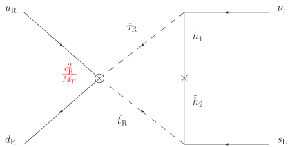
Figure 6: Proton decay, $p\to K^{+}\overline{\nu}_{\tau}$, through dimension 5 RRRR operator.

In fact these contributions from dimension 5 operators are extremely dangerous. From the bound on the proton lifetime we have that, for $\tan\beta=2.5$ and $m_{\tilde{f}}\raise 1.29167pt\hbox{$\;<$\kern-7.5pt\raise-4.73611pt\hbox{$\sim\;$}}1$ TeV

$$M_{T}\geq 6.5\times 10^{16}\mbox{GeV},$$ (58)

and this bound becomes more severe for larger values of $\tan\beta$ given that the RRRR amplitude scales as $\tan^{2}\beta/M_{T}$. On the other hand, in minimal $SU(5)$, there is an upper bound on the Higgs triplet mass if we require correct gauge coupling unification, $M_{T}\leq 2.5\times 10^{16}$ GeV at $90\%$ C.L.. This implies that the minimal SUSY SU(5) model would be excluded by proton decay if the sfermion masses are smaller than 1 TeV. Obviously, much in the same way that non-SUSY GUTs can be complicated enough to avoid the too fast proton decay present in minimal $SU(5)$, also in the SUSY case it is possible to avoid the mentioned problem in the minimal $SU(5)$ realisation by going to non-minimal SU(5) realisations or changing the gauge group altogether. How “realistic” such non-minimal SUSY-GUTs are is what we shortly discuss in the next subsection.

2.3.2 “Realistic” supersymmetric $SU(5)$ models

Gauge coupling unification in supersymmetric grand unified theories is a big quantitative success. However, minimal $SU(5)$ models, face a series of other problems like proton decay or doublet-triplet splitting. A sufficiently “realistic” model should be able to address and solve all these problems simultaneously [50]. The problems we would like this model to solve are: i) gauge coupling unification with an acceptable value of $\alpha_{s}(M_{Z})$ given $\alpha$ and $\sin^{2}\theta_{W}$ at $M_{Z}$, ii) compatibility with the very stringent bounds on proton decay and iii) natural doublet-triplet splitting.

To solve the doublet-triplet problem we use the missing partner mechanism presented above. The superpotential of this model will be that of Eq. (52) with the addition of the Yukawa couplings. Now the $SU(5)$ symmetry is broken to the SM by a VEV of the representation ${\bf 75}$. This provides a mass for the Higgs triplets while the doublets remain massless. Later a $\mu$-term for the Higgs doublets of the order of the electroweak scale is generated through the Giudice-Masiero mechanism [51].

Regarding gauge coupling unification, it is well known that in minimal supersymmetric $SU(5)$ the central value of $\alpha_{3}(M_{Z})$ required by gauge coupling unification is too large: $\alpha_{3}(M_{Z})\simeq 0.13$ to be compared with the experimental value $\alpha_{3}^{\rm exp}(M_{Z})\simeq 0.1187\pm 0.002$. Using two loop RGE equations and taking into account the threshold effects we can write the corrected value of $\alpha_{3}(M_{Z})$ as

$$\alpha_{3}(M_{Z}) = \frac{\displaystyle{\alpha_{3}^{(0)}(M_{Z})}}{\displaystyle{1+\alpha_{3}^{(0)}(M_{Z})~{}\delta}}$$

$$\delta = k+\frac{\displaystyle{1}}{\displaystyle{2\pi}}\log\frac{\displaystyle{M_{\rm SUSY}}}{\displaystyle{M_{Z}}}-\frac{\displaystyle{3}}{\displaystyle{5\pi}}\log\frac{\displaystyle{M_{T}}}{\displaystyle{M_{\mbox{\scriptsize GUT}}}},$$ (59)

with $\alpha_{3}^{(0)}$ the leading log value of this coupling equal to the minimal $SU(5)$ value and $k$ contains the contribution from two loop running, SUSY and GUT thresholds. $M_{T}$ is an effective mass defined as

$$m_{T}=\frac{\displaystyle{M_{T_{1}}M_{T_{2}}}}{\displaystyle{\tilde{M}}},$$ (60)

with $M_{T_{1}}$ and $M_{T_{1}}$ the two eigenvalues of the Higgs triplet mass matrix and $\tilde{M}$ the mass of the ${\bf 50}$ in the superpotential, Eq. (53). The value of the parameter $k$ is different in the minimal $SU(5)$ model and in the realistic model with a ${\bf 75}$ breaking the $SU(5)$ symmetry:

$$k^{\rm minimal}=-1.243 k^{\rm realistic}=0.614\ .$$ (61)

This difference is very important and improves substantially the comparison of the prediction with the experimental value of $\alpha_{3}(M_{Z})$. In fact, for $k$ large and negative we need to take $M_{\rm SUSY}$ as large as possible and $M_{T}$ as small as possible, but this runs into problems with proton decay. On the other hand if $k$ is positive and large, we can take $M_{T}>M_{\mbox{\scriptsize GUT}}$. For instance, with $M_{T}=6\times 10^{17}{\rm GeV}\simeq 30M_{\mbox{\scriptsize GUT}}$ and $M_{\rm SUSY}=0.25$ TeV we obtain $\alpha_{3}(M_{Z})\simeq 0.116$ which is acceptable.

Regarding proton decay the main contribution comes again from dimension five operators when the Higgs triplets are integrated out. Clearly these operators depend on $M_{T}$, but we have seen above that a large $M_{T}$ is preferred in this model. Typical values would be

$$M_{\mbox{\scriptsize GUT}}=2.9\times 10^{16}{\rm GeV},\qquad\tilde{M}=2.0\times 10^{16}{\rm GeV},\qquad~{}$$ (62)

$$M_{T_{1}}=1.2\times 10^{17}{\rm GeV},~{}~{}M_{T_{2}}=1.0\times 10^{17}{\rm GeV},~{}~{}M_{T}=6\times 10^{17}{\rm GeV}.$$

Notice that in this case the couplings of the triplets to the fermions is not related to the fermion masses as the Higgs triplets are now a mixing between the triplets in the ${\bf 5_{H}}$ and the triplets in the ${\bf 50}$. Therefore we have some unknown Yukawa coupling $Y_{\bf\bar{5}0}$. Assuming a hierarchical structure in these couplings somewhat analogous to the doublet Yukawa couplings [50] we would obtain a proton decay rate in the range $8\times 10^{31}$– $3\times 10^{34}$ yrs for the channel $p\to K^{+}\overline{\nu}$ and $2\times 10^{32}$– $8\times 10^{34}$ yrs for the channel $p\to\pi^{+}\overline{\nu}$. The present bound at $90\%$ C.L. on $\tau/{\rm BR}(p\to K^{+}\overline{\nu})$ is $1.9\times 10^{33}$ yrs. Thus we see that agreement with the stringent proton decay bounds is possible in this model.

2.4 Other GUT Models

So, far we have discussed $SU(5)$, the prototype Grand Unified theory in both supersymmetric and non-supersymmetric versions. Given that supersymmetric Grand Unification ensures gauge coupling unification, most models of Grand Unification which have been studied in recent years have been supersymmetric. Other than the SUSY SU(5), historically, one of the first unified models constructed was the Pati-Salam model [24]. The gauge group was given by, $SU(4)_{c}\times SU(2)_{L}\times SU(2)_{R}$. The fermion representations, as explained above, require the presence of a right-handed neutrino. Realistic models can be built incorporating bi-doublets of Higgs giving rise to fermion masses and suitable representations for the breaking of the gauge group. However the Pati-Salam Model is not truly a unified model in a strict sense. For this reason, one needs to go for a larger group of which the Pati-Salam gauge group would be a sub-group. The simplest gauge group in this category is an orthogonal group $SO(10)$ of rank 5.

2.4.1 The seesaw mechanism

There are several reasons to consider models beyond the simple $SU(5)$ gauge group we have considered here. One of the major reasons is the question of neutrino masses. This can be elegantly be solved through a mechanism which goes by the name seesaw mechanism [52, 53, 54, 55, 56]. The seesaw mechanism requires an additional standard model singlet fermion, which could be the right handed neutrino. Given that it is electrically neutral, this particle can have a Majorana mass (violating lepton number by two units) in addition to the standard Dirac mass that couples it to the SM left handed neutrino. Representing the three left-handed fields by a column vector $\nu_{L}$ and the three right handed fields by $\nu_{R}$, the Dirac mass terms are given by

$$-{\mathcal{L}}^{D}=\bar{\nu}_{L}{\cal M}_{D}\nu_{R}+{\rm H.C.},$$ (63)

where ${\cal M}^{D}$ represents the Dirac mass matrix. The Majorana masses for the right handed neutrinos are given by

$$-{\mathcal{L}}^{R}={1\over 2}\bar{\nu}_{R}^{c}{\cal M}_{R}\nu_{R}+{\rm H.C.}.$$ (64)

The total mass matrix is given as

$$-{\mathcal{L}}^{total}={1\over 2}\bar{\nu}_{p}{\cal M}\nu_{p},$$ (65)

where the column vector $\nu_{p}$ is

$$\nu_{p}=\left(\begin{array}[]{c}\nu_{L}\\ \nu_{R}^{c}\end{array}\right).$$ (66)

And the matrix ${\cal M}$ is

$${\cal M}=\left(\begin{array}[]{cc}0&{\cal M}_{D}^{T}\\ {\cal M}_{D}&{\cal M}_{R}\end{array}\right).$$ (67)

Diagonalising the above matrix, one sees that the left handed neutrinos attain Majorana masses of order,

$${\cal M}^{\nu}=-{\cal M}_{D}^{T}~{}{\cal M}_{R}^{-1}{\cal M}_{D}.$$ (68)

This is called the seesaw mechanism. Choosing for example the Dirac mass of the neutrinos to be typically of the order of charged lepton masses or down quark masses, we see that for a heavy right handed neutrino mass scale (${\cal M}_{R}\gg{\cal M}_{D}$), the left-handed neutrino masses are highly suppressed. In this way, the smallness of neutrino masses can be explained naturally by the seesaw mechanism. While the seesaw mechanism is elegant, as mentioned in the Introduction, by construction we do not have right handed neutrinos in the SM particle spectrum. The $SU(5)$ representations do not contain a right handed singlet particle either, as we have seen above. However, in larger GUT groups like $SO(10)$ these additional particles are naturally present.

2.4.2 SO(10)

The group theory of $SO(10)$ and its spinorial representations can be simplified by using the $SU(N)$ basis for the $SO(2N)$ generators or the tensorial approach. The spinorial representation of the $SO(10)$ is given by a 16-dimensional spinor, which could accommodate all the SM model particles as well as the right handed neutrino. The question of gauge coupling unification in $SO(10)$ is more complicated as now there is a ‘natural’ possibility of an intermediate scale. Rest assured it can be achieved, though it depends on the $SO(10)$ breaking mechanism chosen.

Let’s now see how fermions attain their masses in this model. The product of two 16 matter representations can only couple to 10, 120 or 126 representations, which can be formed by either a single Higgs field or a non-renormalisable product of representations of several Higgs fields. In either case, the Yukawa matrices resulting from the couplings to 10 and 126 are complex-symmetric, whereas they are antisymmetric when the couplings are to the 120. Thus, the most general $SO(10)$ superpotential relevant to fermion masses can be written as

$$W_{SO(10)}=h^{10}_{ij}{\bf 16_{i}}~{}{\bf 16_{j}}~{}{\bf 10}+h^{126}_{ij}{\bf 16_{i}}~{}{\bf 16_{j}}~{}{\bf 126}+h^{120}_{ij}{\bf 16_{i}}~{}{\bf 16_{j}}~{}{\bf 120},$$ (69)

where $i,j$ refer to the generation indices. In terms of the SM fields, the Yukawa couplings relevant for fermion masses are given by [57, 30] :

$${\bf 16}\ {\bf 16}\ {\bf 10}\ \supset {\bf 5}\ (uu^{c}+\nu\nu^{c})+{\bf\bar{5}}\ (dd^{c}+ee^{c}),$$ (70)

$${\bf 16}\ {\bf 16}\ {\bf 126}\ \supset {\bf 1}\ \nu^{c}\nu^{c}+15\ \nu\nu+{\bf 5}\ (uu^{c}-3~{}\nu\nu^{c})+{\bf\bar{45}}\ (dd^{c}-3~{}ee^{c}),$$

$${\bf 16}\ {\bf 16}\ {\bf 120}\ \supset {\bf 5}\ \nu\nu^{c}+{\bf 45}\ uu^{c}+{\bf\bar{5}}\ (dd^{c}+ee^{c})+{\bf\bar{45}}\ (dd^{c}-3~{}ee^{c}),$$

where we have specified the corresponding $SU(5)$ Higgs representations for each of the couplings and all the fermions are left handed fields. The resulting mass matrices can be written as

$$M^{u} = M^{5}_{10}+M^{5}_{126}+M^{45}_{120},$$ (71)

$$M^{\nu}_{LR} = M^{5}_{10}-3~{}M^{5}_{126}+M^{5}_{120},$$ (72)

$$M^{d} = M^{\bar{5}}_{10}+M^{\bar{45}}_{126}+M^{\bar{5}}_{120}+M^{\bar{45}}_{120},$$ (73)

$$M^{e} = M^{\bar{5}}_{10}-3M^{\bar{45}}_{126}+M^{\bar{5}}_{120}-3M^{\bar{45}}_{120},$$ (74)

$$M^{\nu}_{LL} = M^{15}_{126},$$ (75)

$$M^{\nu}_{R} = M^{1}_{126}.$$ (76)

We can see here the relations between the different fermionic species. In particular, notice the relation between up-quarks and neutrino (Dirac) mass matrices, Eqs. (71) and (72).

The breaking of $SO(10)$ to the Standard Model group on the other hand can be quite complex compared to that of the $SU(5)$ model we have studied so far. In particular, the gauge group offers the possibility of the existence of an intermediate scale where another “gauge symmetry”, a subgroup of $SO(10)$, can exist. Some of the popular ones are summarised in the figure below:

Figure 7: The various breaking chains of $SO(10)$ are summarised in this figure.

Each of these breaking chains would have its own RG scaling which can in principle lead to different results at the weak scale even though the initial conditions at the $SO(10)$ scale are the same. Different Higgs representations are used for the breaking in each of these cases. In the recent years, attempts have been made to construct complete (renormalisable) models of $SO(10)$ where it could be possible to have precision studies of $SO(10)$ models. This studies do give a good handle on the predictions on proton life time, gauge coupling unification, and, to some extent, fermion masses. However, for processes involving the supersymmetric spectra like flavour changing neutral currents, etc, the situation is more model dependent.

Apart from $SU(5)$ and $SO(10)$, there are other GUT models in the literature based on gauge groups $E_{6}$, $SU(6)$ etc, which we have not touched in this set of lectures.

3 FLAVOUR AND CP VIOLATION IN SUSY

Before entering into the issues of flavour in supersymmetric GUTs, it is instructive to study the issue of flavour within SUSY Standard Models. The simplest Supersymmetric version of the Standard Model that we can build is the so-called Minimal Supersymmetric Standard Model (MSSM). Clearly, this model must include all the SM interactions and particle spectrum together with their Supersymmetric partners. This means that to every quark and lepton in the SM we add a scalar Supersymmetric partner, called “squark” or “slepton” respectively, with identical gauge quantum numbers and, in principle, identical mass, forming a “chiral supermultiplet”. In the same way, to the SM Higgs or more exactly to the Higgses in a 2 Higgs doublet version of the SM we add fermionic partners called “higgsinos” with the same quantum numbers and masses in another “chiral Supermultiplet”. Then every gauge boson is also joined by a gaugino (“gluino”, “wino”, “bino”…) with spin $1/2$ in the adjoint representation in a “vector supermultiplet” (for a complete formulation of Supersymmetric theories in superfield notation see Ref. [59]).

The gauge interactions in our MSSM are completely fixed by the gauge quantum numbers of the different particles in the usual way. However, we still need the Yukawa interactions of the Standard Model that give masses to the fermions once we break the electroweak symmetry. These interactions are included in the MSSM Superpotential, which is a gauge invariant analytic function of the MSSM superfields (i.e. a function of fields $\phi_{i}$ but not of complex conjugate fields $\phi_{i}^{*}$) with dimensions of mass cube. If we include all possible terms invariant under the gauge symmetry then it turns out that some of these terms violate either baryon or lepton number. As we have seen in the previous section, this endangers proton stability; hence one usually imposes a discrete symmetry called R-parity under which the ordinary particles are even while their SUSY partners are odd [60] . The MSSM Superpotential (using standard notation) is then,

$$W=Y_{d}^{ij}Q_{i}H_{1}d^{c}_{Rj}+Y_{e}^{ij}L_{i}H_{1}e^{c}_{Rj}+Y_{u}^{ij}Q_{i}H_{2}u^{c}_{Rj}+\mu H_{1}H_{2},$$ (77)

and this gives rise to the interactions,

$${\mathcal{L}}_{W}=\left|\frac{\displaystyle{\partial W}}{\displaystyle{\partial\phi_{i}}}\right|^{2}+\psi_{i}\psi_{j}\frac{\displaystyle{\partial^{2}W}}{\displaystyle{\partial\phi_{i}\partial\phi_{j}}},$$ (78)

with $\phi_{i}$ any scalar in the MSSM and $\psi_{i}$ its corresponding fermionic partner.

Still, we know that Supersymmetry is not an exact symmetry in nature and it must be broken. If Supersymmetry is the solution to the hierarchy problem, the breaking of Supersymmetry must be soft, i.e. should not reintroduce the quadratic divergences which are forbidden in the SUSY invariant case, and the scale of SUSY breaking must be close to the electroweak scale. The most general set of possible Soft SUSY breaking terms (SBT) [41] under these conditions are,

1. Gaugino masses
   ${\mathcal{L}}_{\mbox{\scriptsize soft}}^{(1)}=\frac{\displaystyle{1}}{\displaystyle{2}}\left(M_{1}\ \tilde{B}\tilde{B}+M_{2}\ \tilde{W}\tilde{W}+M_{3}\ \tilde{g}\tilde{g}\right)+$ h.c.

2. Scalar masses
   ${\mathcal{L}}_{\mbox{\scriptsize soft}}^{(2)}=(M_{\tilde{Q}}^{2})_{ij}\tilde{Q}_{i}\tilde{Q}_{j}^{*}+(M_{\tilde{u}}^{2})_{ij}\tilde{u}_{Ri}^{c}\tilde{u}_{Rj}^{c*}+(M_{\tilde{d}}^{2})_{ij}\tilde{d}_{Ri}^{c}\tilde{d}_{Rj}^{c*}+(M_{\tilde{L}}^{2})_{ij}\tilde{L}_{i}\tilde{L}_{j}^{*}+$
   $~{}~{}~{}~{}~{}~{}~{}~{}~{}~{}~{}(M_{\tilde{e}}^{2})_{ij}\tilde{e}_{Ri}^{c}\tilde{e}_{Rj}^{c*}+(m_{H_{1}}^{2})H_{1}H_{1}^{*}+(m_{H_{2}}^{2})H_{2}H_{2}^{*}$

3. Trilinear couplings and B–term
   ${\mathcal{L}}_{\mbox{\scriptsize soft}}^{(3)}=(Y^{A}_{d})^{ij}\tilde{Q}_{i}H_{1}\tilde{d}_{Rj}+(Y^{A}_{e})^{ij}\tilde{L}_{i}H_{1}\tilde{e}^{c}_{Rj}+(Y^{A}_{u})^{ij}\tilde{Q}_{i}H_{2}\tilde{u}^{c}_{Rj}+B\mu H_{1}H_{2}$

where, $M_{\tilde{Q}}^{2}$, $M_{\tilde{u}}^{2}$, $M_{\tilde{d}}^{2}$, $M_{\tilde{L}}^{2}$ and $M_{\tilde{e}}^{2}$ are hermitian $3\times 3$ matrices in flavour space, while $(Y^{A}_{d})$, $(Y^{A}_{u})$ and $(Y^{A}_{u})$ are complex $3\times 3$ matrices and $M_{1}$, $M_{2}$, $M_{3}$ denote the Majorana gaugino masses for the $U(1)$, $SU(2)$, $SU(3)$ gauge symmetries respectively.

This completes the definition of the MSSM. However, these conditions include a huge variety of models with very different phenomenology specially in the flavour and CP violation sectors.

It is instructive to identify all the observable parameters in a general MSSM [62]. Here we distinguish the flavour independent sector which includes the gauge and Higgs sectors and the flavour sector involving the three generations of chiral multiplets containing the SM fermions and their Supersymmetric partners.

In the flavour independent sector, we have three real gauge couplings, $g_{i}$, and three complex gaugino masses, $M_{i}$. In the Higgs sector, also flavour independent, we have a complex $\mu$ parameter in the superpotential, a complex $B\mu$ soft term and two real squared soft masses $m_{H_{1}}^{2}$ and $m_{H_{2}}^{2}$. However, not all the phases in these parameters are physical [63]. In the limit of $\mu=B\mu=0$, vanishing gaugino masses and zero trilinear couplings, $Y^{A}$, (we will discuss trilinear terms in the flavour dependent sector), our theory has two global $U(1)$ symmetries: $U(1)_{R}$ and $U(1)_{PQ}$. This implies that we can use these two global symmetries to remove two of the phases of these parameters. For instance, we can choose a real $B\mu$ and a real gluino mass $M_{3}$. Then, in the flavour independent sector, we have 10 real parameters ($g_{i}$, $|M_{i}|$, $|\mu|$, $B\mu$, $m_{H_{1}}^{2}$ and $m_{H_{2}}^{2}$) and 3 phases ($\mbox{arg}(\mu)$, $\mbox{arg}(M_{1})$ and $\mbox{arg}(M_{2}))$.

Next, we have to analyse the flavour dependent sector. As a starting point, let us not take into account the non-zero neutrino masses. Then, in the superpotential we have the up quark, down quark and charged lepton Yukawa couplings, $Y_{u}$, $Y_{d}$ and $Y_{e}$, that are complex $3\times 3$ matrices. In the soft breaking sector we have 5 hermitian mass squared matrices, $M_{\tilde{Q}}^{2}$, $M_{\tilde{U}}^{2}$, $M_{\tilde{D}}^{2}$, $M_{\tilde{L}}^{2}$ and $M_{\tilde{E}}^{2}$ and three complex trilinear matrices, $Y^{A}_{u}$, $Y^{A}_{d}$ and $Y^{A}_{e}$. This implies we have $6\times 9$ moduli and $6\times 9$ phases from the 6 complex matrices ($Y_{u}$, $Y_{d}$, $Y_{e}$, $Y^{A}_{u}$, $Y^{A}_{d}$ and $Y^{A}_{e}$) and $5\times 6$ moduli and $5\times 3$ phases from the 5 hermitian matrices. Therefore, in the flavour sector we have 84 moduli and 69 phases. However, it is well-known that not all these parameters are observable. In the absence of these flavour matrices the theory has a global $U(3)_{Q_{L}}\otimes U(3)_{u_{R}}\otimes U(3)_{d_{R}}\otimes U(3)_{L_{L}}\otimes U(3)_{e_{R}}$ flavour symmetry under exchange of the different particles of the three generations. The number of observable parameters is easily determined using the method in Ref. [64] as,

$$N=N_{fl}-N_{G}-N_{G^{\prime}},$$ (79)

where $N_{fl}$ is the number of parameters in the flavour matrices. $N_{G}$ is the number of parameters of the group of invariance of the theory in the absence of the flavour matrices $G=U(3)_{Q_{L}}\otimes U(3)_{u_{R}}\otimes U(3)_{d_{R}}\otimes U(3)_{L_{L}}\otimes U(3)_{e_{R}}$. Finally $N_{G^{\prime}}$ is the number of parameters of the group $G^{\prime}$, the subgroup of $G$ still unbroken by the flavour matrices. In this case, $G^{\prime}$ corresponds to two $U(1)$ symmetries, baryon number conservation and lepton number conservation and therefore $N_{G^{\prime}}=2$. Furthermore Eq. (79) can be applied separately to phases and moduli. In this way, and taking into account that a $U(N)$ matrix contains $n(n-1)/2$ moduli and $n(n+1)/2$ phases, it is straightforward to obtain that we have, $N_{ph}=69-5\times 6+2=41$ phases and $N_{mod}=84-5\times 3=69$ moduli in the flavour sector. This amounts to a total of 123 parameters in the model, out of which 44 are CP violating phases!! As we know, in the SM, there is only one observable CP violating phase, the CKM phase, and therefore we have here 43 new phases, 40 in the flavour sector and three in the flavour independent sector.

Clearly, to explore completely the flavour and CP violating phenomena in a generic MSSM is a formidable task as we have to determine a huge number of unknown parameters [65]. However, this parameter counting corresponds to a completely general MSSM at the electroweak scale but the number of parameters is largely reduced in most of the theory motivated models defined at high energies. In these models most of the parameters at $M_{W}$ are fixed as a function of a handful of parameters at the scale of the transmission of SUSY breaking, for instance $M_{Pl}$ in the case of supergravity mediation, and therefore there are relations among the parameters at $M_{W}$. So, our task will be to determine as many as possible of the CP violating and flavour parameters at $M_{W}$ to look for possible relations among them that will allow us to explore the physics of SUSY and CP breaking at high energies.

The so-called Constrained MSSM (CMSSM), or Sugra-MSSM, (for an early version of these models see, [11, 12]) is the simplest version we can build of the MSSM. For instance a realisation of this model is obtained in string models with dilaton dominated SUSY breaking [66, 67]. Here all the SBT are universal. The soft masses are all proportional to the identity matrix and the trilinear couplings are directly proportional to the corresponding Yukawa matrix. Moreover the gaugino masses are all unified at the high scale. So, we have at $M_{\mbox{\scriptsize GUT}}$,

$$M^{2}_{\tilde{Q}}~{}=~{}M^{2}_{\tilde{U}}~{}=~{}M^{2}_{\tilde{D}}~{}=~{}M^{2}_{\tilde{L}}~{}=~{}M^{2}_{\tilde{E}}~{}=~{}m_{0}^{2}~{}~{}{\hbox{1\kern-2.27621ptl}},$$

$$Y^{A}_{u}=A_{0}~{}Y_{u},\qquad Y^{A}_{d}=A_{0}~{}Y_{d},\qquad Y^{A}_{e}=A_{0}~{}Y_{e},$$

$$m_{H_{1}}^{2}~{}=~{}M_{H_{2}}^{2}~{}=~{}m_{0}^{2}\qquad M_{3}~{}=~{}M_{2}~{}=~{}M_{1}~{}=~{}M_{1/2}$$ (80)

In this way the number of parameters is strongly reduced. If we repeat the counting of parameters in this case we have only 27 complex parameters in the Yukawa matrices, out of which only 12 moduli and 1 phase are observable. In the soft breaking sector we have only a real mass square, $m_{0}^{2}$, and a complex trilinear term, $A_{0}$. We have a single unified gauge coupling, $g_{U}$, and a complex universal gaugino mass $M_{1/2}$ in the gauge sector. Finally in the Higgs sector there are two complex parameters $\mu$ and $B\mu$. Again two of these phases can be reabsorbed through the $U(1)_{R}$ and $U(1)_{PQ}$ symmetries. Therefore, we have only 21 parameters, 18 moduli and 3 phases. In fact, 14 of these parameters are already known in the Standard Model and we are left with only 7 unknown parameters from SUSY: ($m_{0}^{2}$, $|M_{1/2}|$, $|\mu|$, $\mbox{arg}(\mu)$, $|A_{0}|$, $\mbox{arg}(A_{0})$ and $|B|$). If we require radiative electroweak symmetry breaking [68] we get an additional constraint which is used to relate $|B|$ to $M_{W}$. In the literature it is also customary to exchange $|\mu|$ by $\tan\beta=v_{2}/v_{1}$, the ratio of the two Higgs vacuum expectation values, so that the set of parameters usually considered in the MSSM with radiative symmetry breaking is ($m_{0}^{2}$, $|M_{1/2}|$, $\tan\beta$, $|A_{0}|$, $\mbox{arg}(A_{0})$ and $\mbox{arg}(\mu)$). Regarding CP violation, we see that even in the simplest MSSM version we have two new CP violating phases, which we have chosen to be $\varphi_{\mu}\equiv\mbox{arg}(\mu)$ and $\varphi_{A}\equiv\mbox{arg}(A_{0})$. These phases will have a very strong effect on CP violating observables, mainly the Electric Dipole Moments (EDMs) of the electron and the neutron as we will show in the next section. We must remember that a generic MSSM will always include at least these two phases and therefore the constraints from EDMs are always applicable in any MSSM.

All these flavour parameters and phases are encoded at the electroweak scale in the different mass matrices of sfermions and gauginos/higgsinos. For instance, after breaking the $SU(2)_{L}$ symmetry, the superpartners of $W^{\pm}$ and $H^{\pm}$ have the same unbroken quantum number and thus can mix through a matrix,

$$-\frac{\displaystyle{1}}{\displaystyle{2}}\left(\matrix{\tilde{W}^{-}&\tilde{H}_{1}^{-}}\right)\;\left(\matrix{M_{2}&\sqrt{2}M_{W}\sin\beta\cr\sqrt{2}M_{W}\cos\beta&\mu}\right)\left(\matrix{\tilde{W}^{+}\cr\tilde{H}_{2}^{+}}\right),$$ (81)

This non-symmetric (non-hermitian) matrix is diagonalised with two unitary matrices, $U^{*}\cdot M_{\chi^{+}}\cdot V^{\dagger}=\mbox{Diag.}(m_{\chi_{1}^{+}},m_{\chi_{2}^{+}})$.

In the same way, once we break the electroweak symmetry, neutral higgsinos and neutral gauginos mix. In the basis $(\tilde{B}~{}\tilde{W}^{0}\tilde{H}_{1}^{0}\tilde{H}_{2}^{0})$, the mass matrix is,

$$\left(\matrix{M_{1}&0&-M_{Z}c\beta s\theta_{W}&M_{Z}s\beta s\theta_{W}\cr 0&M_{2}&M_{Z}c\beta c\theta_{W}&M_{Z}s\beta c\theta_{W}\cr-M_{Z}c\beta s\theta_{W}&M_{Z}c\beta c\theta_{W}&0&-\mu\cr M_{Z}s\beta s\theta_{W}&-M_{Z}s\beta c\theta_{W}&-\mu&0}\right),$$ (82)

with $c\beta(s\beta)$ and $c\theta_{W}(s\theta_{W})$, $\cos(\sin)\beta$ and $\cos(\sin)\theta_{W}$ respectively. This is diagonalised by a unitary matrix $N$,

$$N^{*}\cdot M_{\tilde{N}}\cdot N^{\dagger}=\mbox{Diag.}(m_{\chi_{1}^{0}},m_{\chi_{2}^{0}},m_{\chi_{3}^{0}},m_{\chi_{4}^{0}})$$ (83)

Finally, the different sfermions, as $\tilde{f}_{L}$ and $\tilde{f}_{R}$, mix after EW breaking. In fact they can also mix with fermions of different generations and in general we have a $6\times 6$ mixing matrix.

$$M_{\tilde{f}}^{2}\;=\;\left(\matrix{m_{\tilde{f}_{\mbox{\scriptsize LL}}}^{2}&m_{\tilde{f}_{\mbox{\scriptsize LR}}}^{2}\cr{m_{\tilde{f}_{\mbox{\scriptsize LR}}}^{2\,\dagger}}&m_{\tilde{f}_{\mbox{\scriptsize RR}}}^{2}}\right)~{}~{}~{}~{}m_{\tilde{f}_{\mbox{\scriptsize LR}}}^{2}\;=\;\big{(}Y^{A}_{f}\cdot^{v_{2}}_{v_{1}}-m_{f}\mu^{\tan\beta}_{\cot\beta}\big{)}\;\;\mbox{for}\;f=^{e,d}_{u}$$

$$m_{\tilde{f}_{\mbox{\scriptsize LL}}}^{2}=M^{2}_{\tilde{f}_{L}}+m^{2}_{f}+M_{Z}^{2}\cos 2\beta(I_{3}+\sin^{2}\theta_{W}Q_{\mbox{\scriptsize em}})$$

$$m_{\tilde{f}_{\mbox{\scriptsize RR}}}^{2}=M^{2}_{\tilde{f}_{R}}+m^{2}_{f}+M_{Z}^{2}\cos 2\beta\sin^{2}\theta_{W}Q_{\mbox{\scriptsize em}}$$ (84)

These hermitian sfermion mass matrices are diagonalised by a unitary rotation,
$R_{\tilde{f}}\cdot M_{\tilde{f}}\cdot R_{\tilde{f}}^{\dagger}=\mbox{Diag.}(m_{\tilde{f}_{1}},m_{\tilde{f}_{2}},\dots,m_{\tilde{f}_{6}})$.

Therefore all the new SUSY phases are kept in these gaugino and sfermion mixing matrices. However, it is not necessary to know the full mass matrices to estimate the CP violation effects. We have some powerful tools as the Mass Insertion (MI) approximation [69, 70, 71, 72] to analyse FCNCs and CP violation. In this approximation, we use flavour diagonal gaugino vertices and the flavour changing is encoded in non-diagonal sfermion propagators. These propagators are then expanded assuming that the flavour changing parts are much smaller than the flavour diagonal ones. In this way we can isolate the relevant elements of the sfermion mass matrix for a given flavour changing process and it is not necessary to analyse the full $6\times 6$ sfermion mass matrix. Using this method, the experimental limits lead to upper bounds on the parameters (or combinations of) $\delta_{ij}^{f}\equiv\Delta^{f}_{ij}/m_{\tilde{f}}^{2}$, known as mass insertions; where $\Delta^{f}_{ij}$ is the flavour-violating off-diagonal entry appearing in the $f=(u,d,l)$ sfermion mass matrices and $m_{\tilde{f}}^{2}$ is the average sfermion mass. In addition, the mass-insertions are further sub-divided into LL/LR/RL/RR types, labelled by the chirality of the corresponding SM fermions. In the following sections we will use both the full mass matrix diagonalisation and this MI formalism to analyse flavour changing and CP violation processes. Now, we will start by studying the EDM calculations and constraints which are common to all Supersymmetric models.

3.1 Electric Dipole Moments in the MSSM

The large SUSY contributions to the electric dipole moments of the electron and the neutron are the main source of the so-called “Supersymmetric CP problem”. This “problem” is present in any MSSM due to the presence of the flavour independent phases $\varphi_{\mu}$ and $\varphi_{A}$. Basically Supersymmetry gives rise to contributions to the EDMs at 1 loop order with no suppression associated to flavour as these phases are flavour diagonal [73, 74, 75, 76, 77, 78]. Taking into account these facts, this contribution can be expected to be much larger than the SM contribution which appears only at three loops and is further suppressed by CKM angles and fermion masses. In fact the SM contribution to the neutron EDM is expected to be of the order of $10^{-32}$ e cm, while the present experimental bounds are $d_{n}\leq 6.3\times 10^{-26}$ e cm (90% C.L.) [79] and $d_{e}\leq 1.6\times 10^{-27}$ e cm (90% C.L.) [80]. As we will show here the Supersymmetric 1 loop contributions to the EDM for SUSY masses below several TeV can easily exceed the present experimental bounds. Therefore, these experiments impose very stringent bounds on $\varphi_{\mu}$ and $\varphi_{A}$.

The typical diagram giving rise to a fermion EDM is shown in Figure 8.

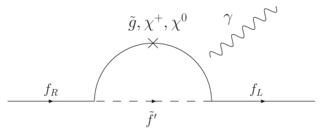
Figure 8: 1 loop contributing to a fermion EDM

In the case of a quark EDM, the dominant contribution typically corresponds to the diagram with internal gluino and squark states. Here all the phases appear only in the squark mass matrix. If we neglect intergenerational mixing (that can be expected to be small), we have a $2\times 2$ squark mass matrix. For instance the down squark mass matrix, $M_{\tilde{d}}$ in the basis $(\tilde{d}_{L},\tilde{d}_{R})$ is,

$$\left(\matrix{m_{\tilde{d}_{L}}^{2}+m_{d}^{2}-(\frac{1}{2}-\frac{1}{3}~{}s^{2}\theta_{W})~{}c2\beta M_{Z}^{2}&Y_{d}^{A\,*}~{}v~{}c\beta-m_{d}~{}\mu~{}tg\beta\cr Y_{d}^{A}~{}v~{}c\beta-m_{d}~{}\mu^{*}~{}tg\beta&m_{\tilde{d}_{R}}^{2}+m_{d}^{2}-\frac{1}{3}~{}s^{2}\theta_{W}~{}c2\beta M_{Z}^{2}}\right)$$ (85)

with $Y_{d}^{A}\simeq A_{0}Y_{d}$ except 1 loop correction in the RGE evolution from $M_{\mbox{\scriptsize GUT}}$ to $M_{W}$. Therefore we have both $\varphi_{\mu}$ and $\varphi_{A}$ in the left-right squark mixing and these phases appear then in the down squark mixing matrix, $R^{d}$, $R^{\tilde{d}}M_{\tilde{d}}R^{\tilde{d}\,\dagger}=\mbox{Diag.}(m_{\tilde{d}_{1}},m_{\tilde{d}_{2}})$. In terms of this mixing matrix the 1 loop gluino contribution to the EDM of the down quark is (in a similar way we would obtain the gluino contribution to the up quark EDM),

$$d^{d}_{\tilde{g}}=\frac{2\alpha_{s}e}{9\pi}\sum_{k=1}^{2}\mbox{Im}[R^{\tilde{d}}_{k2}R^{\tilde{d}\,*}_{k1}]\frac{1}{m_{\tilde{g}}}B(\frac{m_{\tilde{g}}^{2}}{m_{\tilde{d}_{k}}^{2}})$$ (86)

with,

$$B(r)=\frac{r}{2(1-r)^{2}}\left(1+r+\frac{2r\log r}{1-r}\right)$$ (87)

It is interesting to obtain the corresponding formula in terms of the $\left(\delta_{11}^{f}\right)_{\mbox{\scriptsize LR}}$ mass insertion. To do this we observe that given a $n\times n$ hermitian matrix $A=A^{0}+A^{1}$ diagonalised by $U\cdot A\cdot U^{\dagger}=\mbox{Diag}(a_{1},\dots,a_{n})$, with $A^{0}=\mbox{Diag}(a_{1}^{0},\dots,a_{n}^{0})$ and $A^{1}$ completely off-diagonal, we have at first order in $A^{1}$ [81, 82],

$$U_{ki}^{*}f(a_{k})U_{kj}\simeq\delta_{ij}f(a^{0}_{i})+A^{1}_{ij}\frac{\displaystyle{f(a^{0}_{i})-f(a^{0}_{j})}}{\displaystyle{a^{0}_{i}-a^{0}_{j}}}$$ (88)

Therefore, for small off-diagonal entries $A^{1}$ and taking into account that for approximately degenerate squarks we can replace the finite differences by the derivative of the function, $B^{\prime}(x)$, Eq. (86) is converted into,

$$d^{d}_{\tilde{g}} \simeq \frac{2\alpha_{s}e}{9\pi}\frac{m_{\tilde{g}}}{m_{\tilde{d}}^{2}}B^{\prime}(\frac{m_{\tilde{g}}^{2}}{m_{\tilde{d}}^{2}})~{}\mbox{Im}\left[\frac{Y_{d}^{A\,*}~{}v\cos\beta-m_{d}~{}\mu\tan\beta}{m_{\tilde{d}}^{2}}\right]$$ (89)

$$\equiv \frac{2\alpha_{s}e}{9\pi}\frac{m_{\tilde{g}}}{m_{\tilde{d}}^{2}}B^{\prime}(\frac{m_{\tilde{g}}^{2}}{m_{\tilde{d}}^{2}})~{}\mbox{Im}\left[\left(\delta_{11}^{d}\right)_{\mbox{\scriptsize LR}}\right]$$

with $m_{\tilde{d}}^{2}$ the average down squark mass. From this equation it is straightforward to obtain a simple numerical estimate. Taking $m_{\tilde{g}}=m_{\tilde{d}}=500$ GeV, $Y^{A}_{d}=A_{0}Y_{d}$ and $\mu\simeq A_{0}\simeq 500$ GeV, we have,

$$d^{d}_{\tilde{g}} \simeq 2.8\times 10^{-20}~{}~{}\mbox{Im}\left[\left(\delta_{11}^{d}\right)_{\mbox{\scriptsize LR}}\right]\mbox{ e cm}$$

$$= 2.8\times 10^{-25}~{}~{}\left(\sin\varphi_{A}-\tan\beta\sin\varphi_{\mu}\right)\mbox{ e cm}$$

where we used $\alpha_{s}=0.12$ and $m_{d}=5$ MeV. Comparing with the experimental bound on the neutron EDM and using, for simplicity the quark model relation $d_{n}=\frac{1}{3}(4d_{d}-d_{u})$, we see immediately that $\varphi_{A}$ and $(\tan\beta~{}\varphi_{\mu})\leq 0.16$. This is a simple aspect of the “supersymmetric CP problem”. As we will see the constraints from the electron EDM give rise to even stronger bounds on these phases.

In addition, we have also contributions from chargino and neutralino loops which are usually subdominant in the quark EDMs but are the leading contribution in the electron EDM. A simple example is the chargino contribution to the electron EDM. The corresponding diagram is shown in Figure 8 with the chargino and sneutrino in the internal lines,

$$d^{e}_{\chi^{+}}=-\frac{\alpha e}{4\pi\sin^{2}\theta_{W}}~{}\frac{m_{e}}{\sqrt{2}M_{W}\cos\beta}\sum_{j=1}^{2}\mbox{Im}[U_{j2}V_{j1}]\frac{m_{\chi^{+}_{j}}}{m_{\tilde{\nu}_{e}}^{2}}A(\frac{m_{\chi_{j}^{+}}^{2}}{m_{\tilde{\nu}_{e}}^{2}})$$ (91)

with,

$$A(r)=\frac{1}{2(1-r)^{2}}\left(3-r+\frac{2\log r}{1-r}\right)$$ (92)

It is also useful to use a technique similar to Eq. (88) to expand the chargino mass matrix. In this case we have to be careful because the chargino mass matrix is not hermitian. However due to the necessary chirality flip in the chargino line we know that the EDM is a function of odd powers of $M_{\chi^{+}}$ [83],

$$\sum_{j=1}^{2}U_{j2}V_{j1}m_{\chi^{+}_{j}}A(m_{\chi_{j}^{+}}^{2})=\sum_{j,k,l=1}^{2}U_{lk}m_{\chi^{+}_{l}}V_{l1}~{}U_{j2}A(m_{\chi^{+}_{j}}^{2})U^{*}_{jk}.$$ (93)

where we have simply introduced an identity $\delta_{lj}=\sum_{k}U_{lk}U^{*}_{jk}$. Now, assuming $M_{W}\ll M_{2},\mu$, we can use Eq. (88) to develop the loop function A(x) as a function of the hermitian matrix $M_{\chi^{+}}M_{\chi^{+}}^{\dagger}$ and we get,

$$d^{e}_{\chi^{+}} \simeq \frac{-\alpha~{}e~{}m_{e}}{4\pi\sin^{2}\theta_{W}}~{}\frac{\mbox{Im}\left[\sum_{k}\left(M_{\chi^{+}}M_{\chi^{+}}^{\dagger}\right)_{2k}\left(M_{\chi^{+}}\right)_{k1}\right]}{\sqrt{2}M_{W}\cos\beta~{}m_{\tilde{\nu}_{e}}^{2}}~{}\frac{\displaystyle{A(r_{1})-A(r_{2})}}{\displaystyle{m_{\chi_{1}^{+}}^{2}-m_{\chi_{2}^{+}}^{2}}}$$ (94)

$$= \frac{-\alpha~{}e~{}m_{e}\tan\beta}{4\pi\sin^{2}\theta_{W}}~{}\frac{\mbox{Im}[M_{2}~{}\mu]}{m_{\tilde{\nu}_{e}}^{2}}~{}\frac{\displaystyle{A(r_{1})-A(r_{2})}}{\displaystyle{m_{\chi_{1}^{+}}^{2}-m_{\chi_{2}^{+}}^{2}}}$$

with $r_{i}=m_{\chi_{i}^{+}}^{2}/m_{\tilde{\nu}_{e}}^{2}$. This structure with three chargino MIs is shown in figure 9.

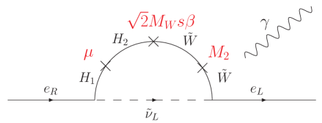
Figure 9: 1 loop chargino contribution to the electron EDM at leading order in chargino mass insertions.

Here we can see that only $\varphi_{\mu}$ enters in the chargino contribution. In fact arg$(M_{2}~{}\mu)$ is the rephasing invariant expression of the observable phase that we usually call $\varphi_{\mu}$. Again we can make a rough estimate with $\mu\simeq M_{2}\simeq m_{\tilde{\nu}}\simeq 200$ GeV (taking the derivative of $A(r)$),

$$d^{e}_{\chi^{+}}\simeq 1.5\times 10^{-25}~{}~{}\tan\beta\sin\varphi_{\mu}\mbox{ e cm}.$$ (95)

Now, comparing with the experimental bound on the electron EDM, we obtain a much stronger bound, $(\tan\beta~{}\varphi_{\mu})\leq 0.01$. These two examples give a clear idea of the strength of the “SUSY CP problem”.

As we have seen in these examples typically the bound on $\varphi_{\mu}$ is stronger than the bound on $\varphi_{A}$. There are several reason for this, as we can see $\varphi_{\mu}$ enters the down-type sfermion mass matrix together with $\tan\beta$ while $\varphi_{A}$ is not enhanced by this factor. Furthermore, $\varphi_{\mu}$ appears also in the chargino and neutralino mass matrices. This difference is increased if we consider the bounds on the original parameters at $M_{\mbox{\scriptsize GUT}}$. The $\mu$ phase is unchanged in the RGE evolution, but $\varphi_{A}=\mbox{arg}(M_{1/2}A_{0})$ (where $M_{1/2}$ is the gaugino mass) is reduced due to large gaugino contributions to the trilinear couplings in the running from $M_{\mbox{\scriptsize GUT}}$ to $M_{W}$. The bounds we typically find in the literature[84, 85] are,

$$\varphi_{\mu}\leq 10^{-2}-10^{-3},~{}~{}~{}~{}~{}~{}~{}~{}\varphi_{A}\leq 10^{-1}-10^{-2}.$$ (96)

Nevertheless, a full computation should take into account all the different contributions to the electron and neutron EDM. In the case of the electron, we have both chargino and neutralino contributions at 1 loop. For the neutron EDM, we have to include also the gluino contribution, the quark chromoelectric dipole moments and the dimension six gluonic operator [86, 87, 88, 89, 90, 84]. When all these contributions are taken into account our estimates above may not be accurate enough and the bound can be loosened.

In fact, there can be regions on the parameter space where different contributions to the neutron or electron EDM have opposite signs and similar size. Thus the complete result for these EDM can be smaller than the individual contributions. In this way, it is possible to reduce the stringent constraints on these phases and $\varphi_{A}={\cal{O}}(1)$ and $\varphi_{\mu}={\cal{O}}(0.1)$ can be still allowed [91, 92, 93, 94, 95, 96, 97]. However, when all the EDM constraints, namely electron, neutron and also mercury atom EDM, are considered simultaneously the cancellation regions practically disappear and the bounds in Eq. (96) remain basically valid [98, 99].

3.2 Flavour changing neutral currents in the MSSM

In the previous section we have analysed the effects of the “flavour independent” SUSY phases, $\varphi_{\mu}$ and $\varphi_{A}$, on the EDMs of the electron and the neutron. However, we have seen that a generic MSSM contains many other observable phases and flavour changing parameters. This huge number of new parameters in the SUSY soft breaking sector can easily generate dangerous contributions in FCNC and flavour changing CP violation processes.

Given the large number of unknown parameters involved in FC processes, it is particularly helpful to make use of the Mass Insertion formalism. The mass insertions are defined in the so-called Super CKM (SCKM) basis. This is the basis where the Yukawa couplings for the down or up quarks are diagonal and we keep the neutral gaugino couplings flavour diagonal. In this basis squark mass matrices are not diagonal and therefore the flavour changing is exhibited by the non-diagonality of the sfermion propagators. Denoting by $\Delta^{f}_{ij}$ the flavour-violating off-diagonal entry appearing in the $f=(u_{L},d_{L},u_{R},d_{R},u_{\mbox{\scriptsize LR}},d_{\mbox{\scriptsize LR}})$ sfermion mass matrices, the sfermion propagators are expanded as a series in terms of $\left(\delta^{f}\right)_{ij}=\Delta^{f}_{ij}/m_{\tilde{f}}$, which are known as mass insertions (MI). Clearly the goodness of this approximation depends on the smallness of the expansion parameter $\delta^{f}_{ij}$. As we will see, indeed the phenomenological constraints require these parameters to be small and it is usually enough to keep the first terms in this expansion. The use of the MI approximation presents the major advantage that it is not necessary to know and diagonalise the full squark mass matrix to perform an analysis of FCNC in a given MSSM. It is enough to know the single entry contributing to a given process and in this way it is easy to isolate the relevant phases.

In terms of the MI, and taking all diagonal elements approximately equal to $m_{\tilde{d}}^{2}$, the down squark mass matrix is,

$$\frac{\displaystyle{M_{\tilde{d}}^{2}}}{\displaystyle{m_{\tilde{d}}^{2}}}\simeq\left(\matrix{1&\left(\delta^{d}_{12}\right)_{\mbox{\scriptsize LL}}&\left(\delta^{d}_{13}\right)_{\mbox{\scriptsize LL}}&\left(\delta^{d}_{11}\right)_{\mbox{\scriptsize LR}}&\left(\delta^{d}_{12}\right)_{\mbox{\scriptsize LR}}&\left(\delta^{d}_{13}\right)_{\mbox{\scriptsize LR}}\cr\left(\delta^{d}_{12}\right)_{\mbox{\scriptsize LL}}^{*}&1&\left(\delta^{d}_{23}\right)_{\mbox{\scriptsize LL}}&\left(\delta^{d}_{21}\right)_{\mbox{\scriptsize LR}}&\left(\delta^{d}_{22}\right)_{\mbox{\scriptsize LR}}&\left(\delta^{d}_{23}\right)_{\mbox{\scriptsize LR}}\cr\left(\delta^{d}_{13}\right)_{\mbox{\scriptsize LL}}^{*}&\left(\delta^{d}_{23}\right)_{\mbox{\scriptsize LL}}^{*}&1&\left(\delta^{d}_{31}\right)_{\mbox{\scriptsize LR}}&\left(\delta^{d}_{32}\right)_{\mbox{\scriptsize LR}}&\left(\delta^{d}_{33}\right)_{\mbox{\scriptsize LR}}\cr\left(\delta^{d}_{11}\right)_{\mbox{\scriptsize LR}}^{*}&\left(\delta^{d}_{21}\right)_{\mbox{\scriptsize LR}}^{*}&\left(\delta^{d}_{31}\right)_{\mbox{\scriptsize LR}}^{*}&1&\left(\delta^{d}_{12}\right)_{\mbox{\scriptsize RR}}&\left(\delta^{d}_{13}\right)_{\mbox{\scriptsize RR}}\cr\left(\delta^{d}_{12}\right)_{\mbox{\scriptsize LR}}^{*}&\left(\delta^{d}_{22}\right)_{\mbox{\scriptsize LR}}^{*}&\left(\delta^{d}_{32}\right)_{\mbox{\scriptsize LR}}^{*}&\left(\delta^{d}_{12}\right)_{\mbox{\scriptsize RR}}^{*}&1&\left(\delta^{d}_{23}\right)_{\mbox{\scriptsize RR}}\cr\left(\delta^{d}_{13}\right)_{\mbox{\scriptsize LR}}^{*}&\left(\delta^{d}_{23}\right)_{\mbox{\scriptsize LR}}^{*}&\left(\delta^{d}_{33}\right)_{\mbox{\scriptsize LR}}^{*}&\left(\delta^{d}_{13}\right)_{\mbox{\scriptsize RR}}^{*}&\left(\delta^{d}_{23}\right)_{\mbox{\scriptsize RR}}^{*}&1\cr}\right),$$ (97)

with all the off-diagonal elements complex which means we have 15 new moduli and 15 phases. The same would be true for the up squark mass matrix, although the $\left(\delta^{u}_{ij}\right)_{\mbox{\scriptsize LL}}$ would be related to $\left(\delta^{d}_{ij}\right)_{\mbox{\scriptsize LL}}$ by a CKM rotation. Therefore there would be a total of 27 moduli and 27 phases in the squark sector.

An illustrative example of the usage of the MI formalism is provided by the SUSY contribution to $K$–$\bar{K}$ [69, 70, 71, 72] mixing.

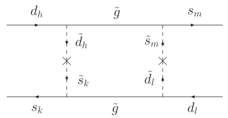
Figure 10: 1 loop contribution to $K$–$\bar{K}$ mixing

The relevant diagram at leading order in the MI approximation is shown in Fig. 10. Here the MI are treated as new vertices in our theory. We have to compute the contribution to the Wilson coefficients of the different four–fermion operators in the $\Delta S=2$ effective Hamiltonian [72, 100]. For example the Wilson coefficient associated with the operator, $Q_{1}=\bar{d}^{\alpha}_{L}\gamma^{\mu}s^{\alpha}_{L}~{}d^{\beta}_{L}\gamma_{\mu}s^{\beta}_{L}$, would be,

$$C_{1}=-\frac{\alpha_{s}^{2}}{216m_{\tilde{q}}^{2}}\left(24xf_{6}(x)+66\tilde{f}_{6}(x)\right)\left(\delta^{d}_{12}\right)_{\mbox{\scriptsize LL}}^{2}$$ (98)

with $x=m_{\tilde{g}}^{2}/m_{\tilde{q}}^{2}$ and the functions $f_{6}(x)$ and $\tilde{f}_{6}(x)$ given by,

$$f_{6}(x)=\frac{6(1+3x)\log x+x^{3}-9x^{2}-9x+17}{6(x-1)^{5}}$$

$$\tilde{f}_{6}(x)=\frac{6x(1+x)\log x-x^{3}-9x^{2}+9x+1}{3(x-1)^{5}}.$$ (99)

It is straightforward to understand the different factors in this formula: we have four flavour diagonal gluino vertices providing a factor $g_{s}^{4}$ and the two MI which supply the necessary flavour transition. The remainder corresponds only to the loop functions. A full computation of the whole set of Wilson coefficients can be found in Refs. [72, 100].

The complete leading order expression for $K^{0}$–$\bar{K}^{0}$ mixing, using the Vacuum Insertion Approximation (VIA) for the matrix elements of the different operators, is [72],

$$\langle K^{0}|{\mathcal{H}}_{\mbox{\scriptsize eff}}^{\Delta S=2}|\bar{K}^{0}\rangle = -\frac{\alpha_{s}^{2}}{216m_{\tilde{q}}^{2}}~{}\frac{1}{3}m_{K}f_{K}^{2}\left\{\right.$$

$$\left.\left(\left(\delta^{d}_{12}\right)_{\mbox{\scriptsize LL}}^{2}+\left(\delta^{d}_{12}\right)_{\mbox{\scriptsize RR}}^{2}\right)\left(24xf_{6}(x)+66\tilde{f}_{6}(x)\right)\right.$$

$$+ \left.\left(\delta^{d}_{12}\right)_{\mbox{\scriptsize LL}}\left(\delta^{d}_{12}\right)_{\mbox{\scriptsize RR}}\left[\left(84\left(\frac{m_{K}}{m_{s}+m_{d}}\right)^{2}+72\right)xf_{6}(x)\right.\right.$$

$$\qquad\qquad\qquad+\left.\left.\left(-24\left(\frac{m_{K}}{m_{s}+m_{d}}\right)^{2}+36\right)\tilde{f}_{6}(x)\right]\right.$$

$$+ \left.\left(\left(\delta^{d}_{12}\right)_{\mbox{\scriptsize LR}}^{2}+\left(\delta^{d}_{12}\right)_{\mbox{\scriptsize RL}}^{2}\right)\left(-132\left(\frac{m_{K}}{m_{s}+m_{d}}\right)^{2}\right)xf_{6}(x)\right.$$

$$+ \left.\left(\delta^{d}_{12}\right)_{\mbox{\scriptsize LR}}\left(\delta^{d}_{12}\right)_{\mbox{\scriptsize RL}}\left[-144\left(\frac{m_{K}}{m_{s}+m_{d}}\right)^{2}-84\right]\tilde{f}_{6}(x)\right\}$$

The neutral kaon mass difference and the mixing CP violating parameter, $\varepsilon_{K},$ are given by,

$$\Delta M_{K}=2\Re\langle K^{0}|{\mathcal{H}}_{\mbox{\scriptsize eff}}^{\Delta S=2}|\bar{K}^{0}\rangle$$

$$\varepsilon_{K}=\frac{1}{\sqrt{2}\Delta M_{K}}\Im\langle K^{0}|{\mathcal{H}}_{\mbox{\scriptsize eff}}^{\Delta S=2}|\bar{K}^{0}\rangle$$ (101)

To obtain a model independent bound on the different MI, we assume that each time only one of these MI is different from zero neglecting accidental cancellations between different MIs. Moreover, it is customary to consider only the gluino contributions leaving aside other SUSY contributions as chargino, charged Higgs or neutralino. In fact, in the presence of sizable MI, the gluino contribution provides typically a large part of the full SUSY contribution. Barring sizable accidental cancellations between the SM and SUSY contributions a conservative limit on the $\delta$s is obtained by requiring the SUSY contribution by itself not to exceed the experimental value of the observable under consideration.

The different MI bounds for the $\left(\delta^{d}_{12}\right)_{a}$ ($a=$ LL,RR,LR) are presented in Table 1. As can be seen explicitly in Eq. (3.2) gluino contributions are completely symmetrical under the interchange $L\leftrightarrow R$ and therefore the limits on $\left(\delta^{d}_{12}\right)_{\mbox{\scriptsize RR}}$ are equal to those on $\left(\delta^{d}_{12}\right)_{\mbox{\scriptsize LL}}$ and the limits on $\left(\delta^{d}_{12}\right)_{\mbox{\scriptsize RL}}$ to those on $\left(\delta^{d}_{12}\right)_{\mbox{\scriptsize LR}}$. In this table we present the bounds at tree level in the four fermion effective Hamiltonian (TREE), i.e. using directly Eq. (3.2) without any further QCD corrections and we compare them with bounds obtained using the NLO QCD evolution with lattice B parameters in the matrix elements [100]. As we can see, although QCD corrections may change the bounds even a factor 2, the tree level estimates remain valid as order of magnitude bounds.

	$\sqrt{|\Re(\delta^{d}_{12})_{\mbox{\scriptsize LL}}^{2}|}$		$\sqrt{|\Im(\delta^{d}_{12})_{\mbox{\scriptsize LL}}^{2}|}$
$x$	TREE	NLO	TREE	NLO
0.3	$1.4\times 10^{-2}$	$2.2\times 10^{-2}$	$1.8\times 10^{-3}$	$2.9\times 10^{-3}$
1.0	$3.0\times 10^{-2}$	$4.6\times 10^{-2}$	$3.9\times 10^{-3}$	$6.1\times 10^{-3}$
4.0	$7.0\times 10^{-2}$	$1.1\times 10^{-1}$	$9.2\times 10^{-3}$	$1.4\times 10^{-2}$
	$\sqrt{|\Re(\delta^{d}_{12})_{\mbox{\scriptsize LL}}(\delta^{d}_{12})_{\mbox{\scriptsize RR}}|}$		$\sqrt{|\Im(\delta^{d}_{12})_{\mbox{\scriptsize LL}}(\delta^{d}_{12})_{\mbox{\scriptsize RR}}|}$
$x$	TREE	NLO	TREE	NLO
0.3	$1.8\times 10^{-3}$	$8.6\times 10^{-4}$	$2.3\times 10^{-4}$	$1.1\times 10^{-4}$
1.0	$2.0\times 10^{-3}$	$9.6\times 10^{-4}$	$2.6\times 10^{-4}$	$1.3\times 10^{-4}$
4.0	$2.8\times 10^{-3}$	$1.3\times 10^{-3}$	$3.7\times 10^{-4}$	$1.8\times 10^{-4}$
	$\sqrt{|\Re(\delta^{d}_{12})_{\mbox{\scriptsize LR}}^{2}|}$		$\sqrt{|\Im(\delta^{d}_{12})_{\mbox{\scriptsize LR}}^{2}|}$
$x$	TREE	NLO	TREE	NLO
0.3	$3.1\times 10^{-3}$	$2.6\times 10^{-3}$	$4.1\times 10^{-4}$	$3.4\times 10^{-4}$
1.0	$3.4\times 10^{-3}$	$2.8\times 10^{-3}$	$4.6\times 10^{-4}$	$3.7\times 10^{-4}$
4.0	$4.9\times 10^{-3}$	$3.9\times 10^{-3}$	$6.5\times 10^{-4}$	$5.2\times 10^{-4}$

Table 1: Maximum allowed values for $|\Re\left(\delta^{d}_{12}\right)_{AB}|$ and $|\Im\left(\delta^{d}_{12}\right)_{AB}|$, with $A,B=(L,R)$ for an average squark mass $m_{\tilde{q}}=500$ GeV and for different values of $x=m_{\tilde{g}}^{2}/m_{\tilde{q}}^{2}$. The bounds are given at tree level in the effective Hamiltonian and at NLO in QCD corrections as explained in the text. For different values of $m_{\tilde{q}}$ the bounds scale roughly as $m_{\tilde{q}}/500$ GeV.

The main conclusion we can draw from this table is that MI bounds in $s\to d$ transitions are very tight and this is specially true on the imaginary parts. This poses a very stringent constraint in most attempts to build a viable MSSM or any realistic supersymmetric flavour model [101, 102, 103]. Conversely we can say that $s\to d$ transitions are very sensitive to the presence of relatively small SUSY contributions and a deviation from SM predictions here could provide the first indirect sign of SUSY [104, 105].

CP violating supersymmetric contributions can also be very interesting in the B system [106, 107]. Similarly to the previous case, we can build the $\Delta B=2$ effective Hamiltonian to obtain the bounds from $B_{d}$–$\bar{B}_{d}$ mixing. A full calculation is presented in Ref. [108], in Table 2 we present the results.

	$|\Re(\delta^{d}_{13})_{\mbox{\scriptsize LL}}|$		$|\Re(\delta^{d}_{13})_{\mbox{LL=RR}}|$
$x$	TREE	NLO	TREE	NLO
0.25	$4.9\times 10^{-2}$	$6.2\times 10^{-2}$	$3.1\times 10^{-2}$	$1.9\times 10^{-2}$
1.0	$1.1\times 10^{-1}$	$1.4\times 10^{-1}$	$3.4\times 10^{-2}$	$2.1\times 10^{-2}$
4.0	$6.0\times 10^{-1}$	$7.0\times 10^{-1}$	$4.7\times 10^{-2}$	$2.8\times 10^{-2}$
	$|\Im(\delta^{d}_{13})_{\mbox{\scriptsize LL}}|$		$|\Im(\delta^{d}_{13})_{\mbox{LL=RR}}|$
$x$	TREE	NLO	TREE	NLO
0.25	$1.1\times 10^{-1}$	$1.3\times 10^{-1}$	$1.3\times 10^{-2}$	$8.0\times 10^{-3}$
1.0	$2.6\times 10^{-1}$	$3.0\times 10^{-1}$	$1.5\times 10^{-2}$	$9.0\times 10^{-3}$
4.0	$2.6\times 10^{-1}$	$3.4\times 10^{-1}$	$2.0\times 10^{-2}$	$1.2\times 10^{-2}$
	$|\Re(\delta^{d}_{13})_{\mbox{\scriptsize LR}}|$		$|\Re(\delta^{d}_{13})_{\mbox{LR=RL}}|$
$x$	TREE	NLO	TREE	NLO
0.25	$3.4\times 10^{-2}$	$3.0\times 10^{-2}$	$3.8\times 10^{-2}$	$2.6\times 10^{-2}$
1.0	$3.9\times 10^{-2}$	$3.3\times 10^{-2}$	$8.3\times 10^{-2}$	$5.2\times 10^{-2}$
4.0	$5.3\times 10^{-2}$	$4.5\times 10^{-2}$	$1.2\times 10^{-1}$	$-$
	$|\Im(\delta^{d}_{13})_{\mbox{\scriptsize LR}}|$		$|\Im(\delta^{d}_{13})_{\mbox{LR=RL}}|$
$x$	TREE	NLO	TREE	NLO
0.25	$7.6\times 10^{-2}$	$6.6\times 10^{-2}$	$1.5\times 10^{-2}$	$9.0\times 10^{-3}$
1.0	$8.7\times 10^{-2}$	$7.4\times 10^{-2}$	$3.6\times 10^{-2}$	$2.3\times 10^{-2}$
4.0	$1.2\times 10^{-1}$	$1.0\times 10^{-1}$	$2.7\times 10^{-1}$	$-$

Table 2: Maximum allowed values for $|\Re\left(\delta^{d}_{13}\right)_{AB}|$ and $|\Im\left(\delta^{d}_{13}\right)_{AB}|$, with $A,B=(L,R)$ for an average squark mass $m_{\tilde{q}}=500$ GeV and different values of $x=m_{\tilde{g}}^{2}/m_{\tilde{q}}^{2}$. with NLO evolution and lattice $B$ parameters, denoted by NLO. The missing entries correspond to cases in which no constraint was found for $|\left(\delta^{d}_{ij}\right)_{AB}|<0.9$.

As we can see here, the constraints in the $B_{d}$ system are less stringent than in the $K$ sector specially in the imaginary parts of the MI which come from $\varepsilon_{K}$ and $\sin 2\beta$ [109, 110, 111, 112]. At first sight this may be surprising as it is well-known that CP violation is more prominent in the B system. To understand this difference we analyse more closely these two observables.

Let us assume that the imaginary part of $K^{0}$–$\bar{K}^{0}$ and $B_{d}^{0}$–$\bar{B}_{d}^{0}$ is entirely provided by SUSY from a single $\left(\delta^{d}_{ij}\right)_{\mbox{\scriptsize LL}}$ MI, while the real part is mostly given by SM loops. The Standard Model contribution to $K^{0}$–$\bar{K}^{0}$ mixing is given by,

$$\langle K^{0}|{\mathcal{H}}_{\mbox{\scriptsize eff}}^{\Delta S=2}|\bar{K}^{0}\rangle=-\frac{\alpha_{\mbox{\scriptsize em}}^{2}}{8M_{W}^{2}\sin^{4}\theta_{W}}~{}\frac{m_{c}^{2}}{M_{W}^{2}}\frac{f_{K}^{2}m_{K}}{3}(V_{cs}V_{cd}^{*})^{2}$$ (102)

Replacing this expression and Eq. (3.2) in Eq. (101) we have,

$$\varepsilon_{K}^{\mbox{\tiny SUSY}}=\frac{\left.\mbox{Im}~{}M_{12}\right|_{\mbox{\tiny SUSY}}}{\left.\sqrt{2}~{}\Delta M_{K}\right|_{\mbox{\tiny SM}}}\simeq\frac{\alpha_{s}^{2}\sin^{2}\theta_{W}}{\alpha_{\mbox{\scriptsize em}}^{2}}~{}\frac{M_{W}^{4}}{M_{\mbox{\tiny SUSY}}^{2}~{}m_{c}^{2}}~{}\frac{\mbox{Im}\left\{(\delta^{d}_{12})_{\mbox{\scriptsize LL}}^{2}\right\}}{\left(V_{cd}V_{cs}^{*}\right)^{2}}$$

$$~{}\frac{8(24xf_{6}(x)+66\tilde{f}_{6}(x))}{216\sqrt{2}}\simeq 12.5\times 84\times\frac{\mbox{Im}\left\{(\delta^{d}_{12})_{\mbox{\scriptsize LL}}^{2}\right\}}{0.05}\times 0.026,$$

$$\varepsilon_{K}^{\mbox{\tiny SUSY}}\leq 2.3\times 10^{-3}\Rightarrow\sqrt{\mbox{Im}\left\{(\delta^{d}_{12})_{\mbox{\scriptsize LL}}^{2}\right\}}\leq 2.0\times 10^{-3}$$ (103)

where we used $x=1$ and $M_{\mbox{\tiny SUSY}}=500$ GeV. In the same way, we can obtain an estimate of the MI bound from the $B^{0}$ CP asymmetries. The gluino and SM contributions to $B^{0}$–$\bar{B}^{0}$ mixing are analogous to Eq. (3.2) and Eq. (102) respectively changing $f_{K}^{2}m_{K}\to f_{B}^{2}m_{B}$, $m_{s}\to m_{b}$, $m_{c}\to m_{t}$ and $(V_{cs}V_{cd}^{*})$ by $(V_{tb}V_{td}^{*})$. Then we have,

$$\left.a_{J/\psi}\right|_{\mbox{\tiny SUSY}}=\frac{\left.\mbox{Im}~{}M_{12}\right|_{\mbox{\tiny SUSY}}}{\left|M_{12}\right|_{\mbox{\tiny SM}}}\simeq\frac{\alpha_{s}^{2}\sin^{2}\theta_{W}}{\alpha_{\mbox{\scriptsize em}}^{2}}~{}\frac{M_{W}^{4}}{M_{\mbox{\tiny SUSY}}^{2}~{}m_{t}^{2}}~{}\frac{\mbox{Im}\left\{(\delta^{d}_{13})_{\mbox{\scriptsize LL}}^{2}\right\}}{\left(V_{tb}V_{td}^{*}\right)^{2}}$$

$$~{}\frac{8(24xf_{6}(x)+66\tilde{f}_{6}(x))}{216}\simeq 12.5\times 0.005\times\frac{\mbox{Im}\left\{(\delta^{d}_{13})_{\mbox{\scriptsize LL}}^{2}\right\}}{(0.008)^{2}}\times 0.037,$$

$$\left.a_{J/\psi}\right|_{\mbox{\tiny SUSY}}\leq 0.74\Rightarrow\sqrt{\mbox{Im}\left\{(\delta^{d}_{13})_{\mbox{\scriptsize LL}}^{2}\right\}}\leq 0.14$$ (104)

From here we see that, although there is a difference due to masses and mixings, $m_{c}^{2}(V_{cs}V_{cd}^{*})^{2}$ versus $m_{t}^{2}(V_{tb}V_{td}^{*})^{2}$, the main reason for the difference in the MI bounds is the experimental sensitivity to CP violation observables. In the kaon system we can measure imaginary contributions to $K$–$\bar{K}$ mixings three orders of magnitude smaller than the real part while in the B system we can only distinguish imaginary contributions if they are of the same order as the mass difference. It is clear that we need much larger MI in the B system that in the K system to have observable effects [104]. On the other hand, as we will show in the next section, in realistic flavour models we expect larger MI in b transitions that in s transitions. Whether the B–system or K–system is more sensitive to SUSY will finally depend on the particular model considered.

Similarly, $b\to s$ transitions can be very interesting in SUSY models [113, 114, 115, 116, 117, 118, 119, 120, 121, 122, 123, 124]. In fact, the only phenomenological constraints in this sector come from the $b\to s\gamma$ process. As we can see in Table 3, the bounds are stringent only for the $(\delta^{d}_{23})_{{\mbox{\scriptsize LR}}}$ while they are very weak for $(\delta^{d}_{23})_{{\mbox{\scriptsize LL}},{\mbox{\scriptsize RR}}}$. A large $(\delta^{d}_{23})_{{\mbox{\scriptsize LL}},{\mbox{\scriptsize RR}},{\mbox{\scriptsize LR}}}$ could have observable effects in several decays like $B\to\Phi K_{S}$ that can still differ from the SM predictions [125, 126].

$x$	${\left|\left(\delta^{d}_{23}\right)_{\mbox{\scriptsize LL}}\right|}$	${\left|\left(\delta^{d}_{23}\right)_{\mbox{\scriptsize LR}}\right|}$
$0.3$	$4.4$	$1.3\times 10^{-2}$
$1.0$	$8.2$	$1.6\times 10^{-2}$
$4.0$	$26$	$3.2\times 10^{-2}$

Table 3: Limits on $|\left(\delta_{13}^{d}\right)|$, from the $b\to s\gamma$ decay, for an average squark mass $m_{\tilde{q}}=500\mbox{GeV}$ and for different values of $x=m_{\tilde{g}}^{2}/m_{\tilde{q}}^{2}$. For different values of $m_{\tilde{q}}$, the limits can be obtained multiplying the ones in the table by $\left(m_{\tilde{q}}(\mbox{GeV})/500\right)^{2}$.

Another interesting CP violating process in SUSY is $\varepsilon^{\prime}/\varepsilon$ [127, 128, 129, 130, 131, 132, 133]. We present the corresponding MI bounds from $\varepsilon^{\prime}/\varepsilon<2.7\times 10^{-3}$ [134, 135] in Table 4.

$x$	${\left|\Im\left(\delta^{d}_{12}\right)_{\mbox{\scriptsize LL}}\right|}$	${\left|\Im\left(\delta^{d}_{12}\right)_{\mbox{\scriptsize LR}}\right|}$
$0.3$	$1.0\times 10^{-1}$	$1.1\times 10^{-5}$
$1.0$	$4.8\times 10^{-1}$	$2.0\times 10^{-5}$
$4.0$	$2.6\times 10^{-1}$	$6.3\times 10^{-5}$

Table 4: Limits from $\varepsilon^{\prime}/\varepsilon<2.7\times 10^{-3}$ on $\Im\left(\delta_{12}^{d}\right)$, for an average squark mass $m_{\tilde{q}}=500\mbox{GeV}$ and for different values of $x=m_{\tilde{g}}^{2}/m_{\tilde{q}}^{2}$. For different values of $m_{\tilde{q}}$, the limits can be obtained multiplying the ones in the table by $\left(m_{\tilde{q}}(\mbox{GeV})/500\right)^{2}$.

This observable is more sensitive to chirality changing MI due to the dominance of the gluonic and electroweak penguin operators. The bounds on $\Im\left(\delta^{d}_{12}\right)_{\mbox{\scriptsize LR}}$ look really tight and in fact these are the strongest bounds attainable on this MI. However, it is important to remember that these off-diagonal LR mass insertions come from the trilinear soft breaking terms which in realistic models are always proportional to fermion masses. Thus this MI typically contains a suppression $m_{s}/M_{\mbox{\tiny SUSY}}\simeq 2\times 10^{-4}$ for $M_{\mbox{\tiny SUSY}}=500$ GeV. So, if we consider this “intrinsic” suppression the bounds are less impressive.

In summary, these MI bounds show the present sensitivity of CP violation experiments to the presence of new phases and flavour structures in the SUSY soft breaking terms. An important lesson we can draw from the stringent bounds in the tables is that, in fact we already posses a crucial information on the enormous (123-dimensional) parameter space of a generic MSSM: most of this parameter space is already now excluded by flavour physics, and indeed the “realistic” MSSM realisation should not depart too strongly from the CMSSM, at least barring significant accidental cancellations.

3.3 Mass Insertion bounds from leptonic processes

In this section, we study the constraints on slepton mass matrices in low energy SUSY imposed by several LFV transitions, namely $l_{i}\rightarrow l_{j}\gamma$, $l_{i}\rightarrow l_{j}l_{k}l_{k}$ and $\mu$–$e$ transitions in nuclei [136]. The present and projected bounds on these processes are summarized in Table 5.

Process	Present Bounds	Expected Future Bounds
BR($\mu\to e\,\gamma$)	$1.2~{}\times~{}10^{-11}$	$\mathcal{O}(10^{-13}-10^{-14})$
BR($\mu\to e\,e\,e$)	$1.1~{}\times~{}10^{-12}$	$\mathcal{O}(10^{-13}-10^{-14})$
BR($\mu\to e$ in Nuclei (Ti))	$1.1~{}\times~{}10^{-12}$	$\mathcal{O}(10^{-18})$
BR($\tau\to e\,\gamma$)	$1.1~{}\times~{}10^{-7}$	$\mathcal{O}(10^{-8})$
BR($\tau\to e\,e\,e$)	$2.7~{}\times~{}10^{-7}$	$\mathcal{O}(10^{-8})$
BR($\tau\to e\,\mu\,\mu$)	$2.~{}\times~{}10^{-7}$	$\mathcal{O}(10^{-8})$
BR($\tau\to\mu\,\gamma$)	$6.8~{}\times~{}10^{-8}$	$\mathcal{O}(10^{-8})$
BR($\tau\to\mu\,\mu\,\mu$)	$2~{}\times~{}10^{-7}$	$\mathcal{O}(10^{-8})$
BR($\tau\to\mu\,e\,e$)	$2.4~{}\times~{}10^{-7}$	$\mathcal{O}(10^{-8})$

Table 5: Present and Upcoming experimental limits on various leptonic processes at 90% C.L.

These processes are mediated by chargino and neutralino loops and therefore they depend on all the parameters entering chargino and neutralino mass matrices. In order to constrain the leptonic MIs $\delta^{ij}$, we will first obtain the spectrum at the weak scale for our SU(5) GUT theory as has been mentioned in detail in section 3. Furthermore, we take all the flavor off-diagonal entries in the slepton mass matrices equal to zero except for the entry corresponding to the MI we want to bound. To calculate the branching ratios of the different processes, we work in the mass eigenstates basis through a full diagonalization of the slepton mass matrix. So, imposing that the contribution of each flavor off-diagonal entry to the rates of the above processes does not exceed (in absolute value) the experimental bounds, we obtain the limits on the $\delta^{ij}$’s, barring accidental cancellations.

The process that sets the most stringent bounds is the $l_{i}\rightarrow l_{j}\gamma$ decay, whose amplitude has the form

$$T=m_{l_{i}}\epsilon^{\lambda}\overline{u}_{j}(p-q)[iq^{\nu}\sigma_{\lambda\nu}(A_{L}P_{L}+A_{R}P_{R})]u_{i}(p)\,,$$ (105)

where $p$ and $q$ are momenta of the leptons $l_{k}$ and of the photon respectively, $P_{R,L}=\frac{1}{2}(1\pm\gamma_{5})$ and $A_{L,R}$ are the two possible amplitudes entering the process. The lepton mass factor $m_{l_{i}}$ is associated to the chirality flip present in this transition. In a supersymmetric framework, we can implement the chirality flip in three ways: in the external fermion line (as in the SM with massive neutrinos), at the vertex through a higgsino Yukawa coupling or in the internal gaugino line together with a chirality change in the sfermion line. The branching ratio of $l_{i}\rightarrow l_{j}\gamma$ can be written as

$$\frac{BR(l_{i}\rightarrow l_{j}\gamma)}{BR(l_{i}\rightarrow l_{j}\nu_{i}\bar{\nu_{j}})}=\frac{48\pi^{3}\alpha}{G_{F}^{2}}(|A_{L}^{ij}|^{2}+|A_{R}^{ij}|^{2})\,,$$

with the SUSY contribution to each amplitude given by the sum of two terms $A_{L,R}=A_{L,R}^{n}+A_{L,R}^{c}$. Here $A_{L,R}^{n}$ and $A_{L,R}^{c}$ denote the contributions from the neutralino and chargino loops respectively.

Type of $\delta^{l}_{12}$	$\mu\to e\,\gamma$	$\mu\to e\,e\,e$	$\mu\to e$ conversion in $Ti$
LL	$6\times 10^{-4}$	$2\times 10^{-3}$	$2\times 10^{-3}$
RR	-	$0.09$	-
LR/RL	$1\times 10^{-5}$	$3.5\times 10^{-5}$	$3.5\times 10^{-5}$

Table 6: Bounds on leptonic $\delta^{l}_{12}$ from various $\mu\to e$ processes. The bounds are obtained by making a scan of $m_{0}$ and $M_{1/2}$ over the ranges $m_{0}<380$ GeV and $M_{1/2}<$160 GeV and varying $\tan\beta$ within $5<\tan\beta<15$. The bounds are rather insensitive to the sign of the $\mu$ mass term.

Even though all our numerical results presented in Tables 6–8 are obtained performing an exact diagonalization of sfermion and gaugino mass matrices, it is more convenient for the discussion to use the expressions for the $l_{i}\rightarrow l_{j}\gamma$ amplitudes in the MI approximation. In particular, we treat both the slepton mass matrix and the chargino and neutralino mass matrix off-diagonal elements as mass insertions. In this approximation, we have the following expressions

$$A^{ij}_{L} = \frac{\displaystyle{\alpha_{2}}}{\displaystyle{4\pi}}\frac{\left(\delta^{l}_{ij}\right)_{{\mbox{\scriptsize LL}}}}{m_{\tilde{l}}^{2}}~{}\Bigg{[}~{}f_{1n}(a_{2})\!+\!f_{1c}(a_{2})\!+\!\frac{\mu M_{2}\tan\beta}{(M_{2}^{2}\!-\!\mu^{2})}\bigg{(}f_{2n}(a_{2},b)\!+\!f_{2c}(a_{2},b)\bigg{)}$$

$$\qquad\quad+\tan^{2}\theta_{W}\,\bigg{(}f_{1n}(a_{1})+\mu M_{1}\tan\beta\bigg{(}\frac{f_{3n}(a_{1})}{m_{\tilde{l}}^{2}}+\frac{f_{2n}(a_{1},b)}{(\mu^{2}\!-\!M_{1}^{2})}\bigg{)}\!\bigg{)}\Bigg{]}$$

$$+ \frac{\displaystyle{\alpha_{1}}}{\displaystyle{4\pi}}~{}\frac{\left(\delta^{l}_{ij}\right)_{{\mbox{\scriptsize RL}}}}{m_{\tilde{l}}^{2}}~{}\left(\frac{M_{1}}{m_{l_{i}}}\right)~{}2~{}f_{2n}(a_{1})\,,$$

$$A^{ij}_{R}=\frac{\alpha_{1}}{4\pi} \!\!\Bigg{(}\!\! \frac{\left(\delta^{l}_{ij}\right)_{{\mbox{\scriptsize RR}}}}{m_{\tilde{l}}^{2}}\left[4f_{1n}(a_{1})+\mu M_{1}\tan\beta\left(\frac{f_{3n}(a_{1})}{m_{\tilde{l}}^{2}}-\frac{2f_{2n}(a_{1},b)}{(\mu^{2}\!-\!M_{1}^{2})}\right)\right]$$

$$+ \frac{\left(\delta^{l}_{ij}\right)_{{\mbox{\scriptsize LR}}}}{m_{\tilde{l}}^{2}}~{}\left(\frac{M_{1}}{m_{l_{i}}}\right)~{}2~{}f_{2n}(a_{1})\Bigg{)}\,,$$

where $\theta_{W}$ is the weak mixing angle, $a_{1,2}=M^{2}_{1,2}/\tilde{m}^{2}$, $b=\mu^{2}/m_{\tilde{l}}^{2}$ and $f_{i(c,n)}(x,y)=f_{i(c,n)}(x)-f_{i(c,n)}(y)$. The loop functions $f_{i}$ are given as

$$f_{1n}(x) = (-17x^{3}+9x^{2}+9x-1+6x^{2}(x+3)\ln x)/(24(1-x)^{5}),$$

$$f_{2n}(x) = (-5x^{2}+4x+1+2x(x+2)\ln x)/(4(1-x)^{4}),$$

$$f_{3n}(x) = (1+9x-9x^{2}-x^{3}+6x(x+1)\ln x)/(3(1-x)^{5}),$$

$$f_{1c}(x) = (-x^{3}-9x^{2}+9x+1+6x(x+1)\ln x)/(6(1-x)^{5}),$$

$$f_{2c}(x) = (-x^{2}-4x+5+2(2x+1)\ln x)/(2(1-x)^{4})\,.$$ (108)

Type of $\delta^{l}_{13}$	$\tau\to e\,\gamma$	$\tau\to e\,e\,e$	$\tau\to e\mu\mu$
LL	$0.15$	$-$	-
RR	-	-	-
LR/RL	$0.04$	$0.5$	-

Table 7: Bounds on leptonic $\delta^{l}_{13}$ from various $\tau\to e$ processes obtained using the same values of SUSY parameters as in Table 6.

Type of $\delta^{l}_{23}$	$\tau\to\mu\,\gamma$	$\tau\to\mu\,\mu\,\mu$	$\tau\to\mu\,e\,e$
LL	$0.12$	-	-
RR	-	-	-
LR/RL	$0.03$	-	0.5

Table 8: Bounds on leptonic $\delta^{l}_{23}$ from various $\tau\to\mu$ processes obtained using the same values of SUSY parameters as in Table 6.

We note that all $\left(\delta^{l}_{ij}\right)_{{\mbox{\scriptsize LL}}}$ contributions with internal chirality flip are $\tan\beta$-enhanced. On the other hand, the only term proportional to $\left(\delta^{l}_{ij}\right)_{{\mbox{\scriptsize LR}}}$ arises from pure $\tilde{B}$ exchange and it is completely independent of $\tan\beta$, as can be seen from Eqs. (3.3) and (3.3). Therefore the phenomenological bounds on $\left(\delta^{l}_{ij}\right)_{{\mbox{\scriptsize LL}}}$ depend on $\tan\beta$ to some extent, while those on $\left(\delta^{l}_{ij}\right)_{{\mbox{\scriptsize LR}}}$ do not. The bounds on LL and RL MIs are expected to approximately fulfill the relation

$$\left(\delta^{l}_{ij}\right)_{{\mbox{\scriptsize LR}}}\simeq\frac{m_{i}}{\tilde{m}}\tan\beta\,\,\left(\delta^{l}_{ij}\right)_{{\mbox{\scriptsize LL}}}\,.$$

This is confirmed by our numerical study.

The $\delta^{d}_{{\mbox{\scriptsize RR}}}$ sector requires some care because of the presence of cancellations among different contributions to the amplitudes in regions of the parameter space. The origin of these cancellations is the destructive interference between the dominant contributions coming from the $\tilde{B}$ (with internal chirality flip and a flavor-conserving LR mass insertion) and $\tilde{B}\tilde{H}^{0}$ exchange [136, 137]. We can see this in the MI approximation if we compare the $\tan\beta$ enhanced terms in the second line of Eq. (3.3) with the $\tan\beta$ enhanced terms in Eq. (3.3). Here the loop function $f_{3}(a_{1})$ corresponds to the pure $\tilde{B}$ contribution while $f_{2n}(a_{1},b)$ represents the $\tilde{B}\tilde{H}^{0}$ exchange. These contributions have different relative signs in Eq. (3.3) and Eq. (3.3) due to the opposite sign in the hypercharge of $SU(2)$ doublets and singlets. Thus, the decay $l_{i}\rightarrow l_{j}\gamma$ does not allow to put an absolute bound on the RR sector. We can still take into account other LFV processes such as $l_{i}\rightarrow l_{j}l_{k}l_{k}$ and $\mu$–$e$ in nuclei. These processes get contributions not only from penguin diagrams (with both photon and Z-boson exchange) but also from box diagrams. Still the contribution of dipole operators, being also $\tan\beta$-enhanced, is dominant. Disregarding other contributions, one finds the relations

$$\frac{Br(l_{i}\!\rightarrow\!l_{j}l_{k}l_{k})}{Br(l_{i}\!\rightarrow\!l_{j}\gamma)}\simeq\!\frac{\alpha_{e}}{3\pi}\left(\!\log\frac{m^{2}_{l_{i}}}{m^{2}_{l_{k}}}\!-\!3\!\right)\,,$$

$$Br(\mu-e{\rm\ in\ Ti})\simeq\,\,\alpha_{e}BR(\mu\rightarrow e\gamma)\,,$$ (109)

which clearly shows that $l_{i}\rightarrow l_{j}\gamma$ is the strongest constraint and gives the more stringent bounds on the different $\delta_{ij}$’s. As we have mentioned above, however, in the case of $\delta^{l}_{{\mbox{\scriptsize RR}}}$ the dominant dipole contributions interfere destructively in regions of parameters, so that $Br(l_{i}\rightarrow l_{j}\gamma)$ is strongly suppressed while $Br(\mu-e\rm{\ in\ nuclei})$ and $Br(l_{i}\rightarrow l_{j}l_{k}l_{k})$ are dominated by monopole penguin (both $\gamma^{*}$ and Z-mediated) and box diagrams. The formulae for these contributions can be found in Ref. [138]. However, given that non-dipole contributions are typically much smaller than dipole ones outside the cancellation region, it follows that the bound on $\delta^{l}_{{\mbox{\scriptsize RR}}}$ from $\mu\to eee$ are expected to be less stringent than the one on $\delta^{l}_{{\mbox{\scriptsize LL}}}$ from $\mu\to e\gamma$ by a factor $\sqrt{\alpha/(8\pi)}~{}1/\tan\beta\simeq 0.02/\tan\beta$, if the experimental upper bounds on the two BRs were the same. This is partly compensated by the fact that the present experimental upper bound on the $BR(\mu\to eee)$ is one order of magnitude smaller than that on $BR(\mu\to e\gamma)$, as shown in Tab. 5. On the other hand, the process $BR(\mu-e\rm{\ in\ nuclei})$ suffers from cancellations through the interference of dipole and non-dipole amplitudes as well. These cancellations prevent us from getting a bound in the RR sector from the $\mu$–$e$ conversion in nuclei now as well as in the future when their experimental sensitivity will be improved. However, the $\mu\rightarrow e\gamma$ and $\mu$–$e$ in nuclei amplitudes exhibit cancellations in different regions of the parameter space so that the combined use of these two constraints produces a competitive or even stronger bound than the one we get from $BR(\mu\rightarrow eee)$ alone [136].

We summarize the different leptonic bounds in tables 6–8. All these bounds are obtained making a scan of $m_{0}$ and $M_{1/2}$ over the ranges $m_{0}<$380 GeV and $M_{1/2}<$160 GeV and therefore correspond to the heaviest possible sfermions. As expected, the strongest bounds for $\delta^{l}_{{\mbox{\scriptsize LL}}}$ and $\delta^{l}_{{\mbox{\scriptsize LR}}}$ come always from $\mu\to e\gamma$, $\tau\to\mu\gamma$ and $\tau\to e\gamma$ processes. In the case of $\delta^{l}_{{\mbox{\scriptsize RR}}}$ we can only obtain a mild bound for $\left(\delta^{l}_{12}\right)_{{\mbox{\scriptsize RR}}}$ from $\mu\to eee$ and there are no bounds for $\left(\delta^{l}_{23}\right)_{{\mbox{\scriptsize RR}}}$ and $\left(\delta^{l}_{13}\right)_{{\mbox{\scriptsize RR}}}$. Notice, however, that does not mean that these LFV processes are not effective to constrain the SUSY parameter space in the presence of RR MIs. For most of the values of $m_{0}$ and $M_{1/2}$ there is no cancellation and the values of these MI are required to be of the order of the LL bounds. Only for those values of $m_{0}$ and $M_{1/2}$ satisfying the cancellation conditions a large value of the RR MI is allowed. Therefore, we must check individually these constraints for fixed values of the SUSY parameters.

3.3.1 $(g-2)_{\mu}$

One of the most stringent flavour conserving constraints in the leptonic sector comes from the measurement of the anomalous magnetic moment of the muon [$a_{\mu}=(g-2)_{\mu}/2$]. This has been measured very precisely in the last few years [139, 140, 141], provides a first hint of physics beyond the SM has been widely discussed in the recent literature. Despite substantial progress both on the experimental and on the theoretical sides, the situation is not completely clear yet (see Ref. [142, 143] for an updated discussion).

Most recent analyses converge towards a $2\sigma$ discrepancy in the $10^{-9}$ range [144, 145]:

$$\Delta a_{\mu}=a_{\mu}^{\rm exp}-a_{\mu}^{\rm SM}\approx(2\pm 1)\times 10^{-9}~{}.$$ (110)

The main SUSY contribution to $a^{\rm MSSM}_{\mu}$ is usually provided by the loop exchange of charginos and sneutrinos. The basic features of the supersymmetric contribution to $a_{\mu}$ are correctly reproduced by the following approximate expression:

$$\frac{a^{\rm MSSM}_{\mu}}{1\times 10^{-9}}\approx 1.5\left(\frac{\tan\beta}{10}\right)\left(\frac{300~{}\rm GeV}{m_{\tilde{\nu}}}\right)^{2}\left(\frac{\mu M_{2}}{m^{2}_{\tilde{\nu}}}\right)~{},$$ (111)

which provides a good approximation to the full one-loop result [146]

The most relevant feature of Eqs. (111) is that the sign of $a^{\rm MSSM}_{\mu}$ is fixed by the sign of the $\mu$ term so that the $\mu>0$ region is strongly favored. This is specially true for the Standard Model prediction which uses the data from $e^{+}e^{-}$ collisions to compute the hadronic vacuum polarization (HVP). This predicts a smaller value than the experimental result by about $3~{}\sigma$. In case one uses the $\tau$ data to compute the HVP, the discrepancy with SM is reduced to about $1~{}\sigma$, but it still favors a positive correction and disfavors strongly a sizable negative contribution. Thus, taking $\mu>0$, the region of parameter space considered in this analysis satisfies the constraint of Eq. (110).

3.4 Grand unification and Flavour

In the previous section, we have seen how flavour can be used to constrain various supersymmetric parameters in generic MSSM. What happens if one has a Grand Unified theory instead of the Standard Model ? Well, the answer to this question crucially depends on the mechanism of transmission of supersymmetry breaking to the visible sector, or more exactly on the scale of the interactions mediating SUSY breaking. In the case, the scale of mediation is much below the scale of Grand Unification, then the soft supersymmetry breaking parameters will not see any effects of Grand Unification on them. On the other hand, if indeed mediation of supersymmetry breaking occurs above the Grand Unification scale, as in supergravity theories then the manner of supersymmetry breaking plays a crucial role in determining the flavour aspects of the theory. Lets consider two representative situations in the following :

3.4.1 SUSY-GUTs and Flavour dependent SUSY breaking

As we have been discussing, in a SUSY-GUT, quarks and leptons sit in same multiplets and are transformed ones into the others through GU symmetry transformations. If the supergravity Lagrangian, and, in particular, its Kähler function are present at a scale larger than the GUT breaking scale, they have to fully respect the underlying gauge symmetry which is the GU symmetry itself. The subsequent SUSY breaking will give rise to the usual soft breaking terms in the Lagrangian. In particular, the sfermion mass matrices, originating from the Kähler potential, will have to respect the underlying GU symmetry. Hence we expect hadron-lepton correlations among entries of the sfermion mass matrices. In other words, the quark-lepton unification seeps also into the SUSY breaking soft sector [147].

One of the striking aspects of this scenario is that the imposition of a GU symmetry on the $\mathcal{L}_{soft}$ entails relevant implications at the weak scale. This is because the flavour violating (FV) mass-insertions do not get strongly renormalised through RG scaling from the GUT scale to the weak scale in the absence of new sources of flavor violation. On the other hand, if such new sources are present, for instance due to the presence of new neutrino Yukawa couplings in SUSY GUTs with a seesaw mechanism for neutrino masses, then one can compute the RG-induced effects in terms of these new parameters. Hence, the correlations between hadronic and leptonic flavor violating MIs survive at the weak scale to a good approximation. As for the flavor conserving (FC) mass insertions (i.e., the diagonal entries of the sfermion mass matrices), they get strongly renormalised, but in a way which is RG computable.

To summarise, in SUSY GUTs where the soft SUSY breaking terms respect boundary conditions which are subject to the GU symmetry to start with, we generally expect the presence of relations among the (bilinear and trilinear) scalar terms in the hadronic and leptonic sectors. Such relations hold true at the (superlarge) energy scale where the correct symmetry of the theory is the GU symmetry. After its breaking, the mentioned relations will undergo corrections which are computable through the appropriate RGE’s which are related to the specific structure of the theory between the GU and the electroweak scale (for instance, new Yukawa couplings due to the presence of right-handed (RH) neutrinos acting down to the RH neutrino mass scale, presence of a symmetry breaking chain with the appearance of new symmetries at intermediate scales, etc.). As a result of such a computable running, we can infer the correlations between the softly SUSY breaking hadronic and leptonic $\delta$ terms at the low scale where we perform our FCNC tests.

Given that a common SUSY soft-breaking scalar term of $\mathcal{L}_{soft}$ at scales close to $M_{\rm Planck}$ can give rise to RG-induced $\delta^{q}$’s and $\delta^{l}$’s at the weak scale, one may envisage the possibility to make use of the FCNC constraints on such low-energy $\delta$’s to infer bounds on the soft breaking parameters of the original supergravity Lagrangian ($\mathcal{L}_{sugra}$). Indeed, for each scalar soft parameter of $\mathcal{L}_{sugra}$ one can ascertain whether the hadronic or the leptonic corresponding bound at the weak scale yields the stronger constraint at the large scale. One can then go through an exhaustive list of the low-energy constraints on the various $\delta^{q}$’s and $\delta^{l}$’s and, then, after RG evolving such $\delta$’s up to $M_{Planck}$, we will establish for each $\delta$ of $\mathcal{L}_{sugra}$ which one between the hadronic and leptonic constraints is going to win, namely which provides the strongest constraint on the corresponding $\delta_{sugra}$ [148].

Consider for example the scalar soft breaking sector of the MSSM:

$$-{\cal L}_{soft} = m_{Q_{ii}}^{2}\tilde{Q}_{i}^{\dagger}\tilde{Q}_{i}+m_{u^{c}_{ii}}^{2}\tilde{u^{c}}_{i}^{\star}\tilde{u^{c}}_{i}+m^{2}_{e^{c}_{ii}}\tilde{e^{c}}_{i}^{\star}\tilde{e^{c}}_{i}+m^{2}_{d^{c}_{ii}}\tilde{d^{c}}^{\star}_{i}\tilde{d^{c}}_{i}$$ (112)

$$+ m_{L_{ii}}^{2}\tilde{L}_{i}^{\dagger}\tilde{L}_{i}+m^{2}_{H_{1}}H^{\dagger}_{1}H_{1}+m^{2}_{H_{2}}H_{2}^{\dagger}H_{2}+A^{u}_{ij}~{}\tilde{Q}_{i}\tilde{u^{c}}_{j}H_{2}$$

$$+ A^{d}_{ij}~{}\tilde{Q}_{i}\tilde{d^{c}}_{j}H_{1}+A^{e}_{ij}~{}\tilde{L}_{i}\tilde{e^{c}}_{j}H_{1}+(\Delta^{l}_{ij})_{LL}\tilde{L}_{i}^{\dagger}\tilde{L}_{j}+(\Delta^{e}_{ij})_{RR}\tilde{e^{c}}_{i}^{\star}\tilde{e^{c}}_{j}$$

$$+ (\Delta^{q}_{ij})_{LL}\tilde{Q}_{i}^{\dagger}\tilde{Q}_{j}+(\Delta^{u}_{ij})_{RR}\tilde{u^{c}}_{i}^{\star}\tilde{u^{c}}_{j}+(\Delta^{d}_{ij})_{RR}\tilde{d^{c}}_{i}^{\star}\tilde{d^{c}}_{j}$$

$$+ (\Delta^{e}_{ij})_{LR}\tilde{e_{L}}_{i}^{\star}\tilde{e^{c}}_{j}+(\Delta^{u}_{ij})_{LR}\tilde{u_{L}}_{i}^{\star}\tilde{u^{c}}_{j}+(\Delta^{d}_{ij})_{LR}\tilde{d_{L}}_{i}^{\star}\tilde{d^{c}}_{j}$$

where we have explicitly written down the various $\Delta$ parameters.

Consider now that $SU(5)$ is the relevant symmetry at the scale where the above soft terms firstly show up. Then, taking into account that matter is organised into the SU(5) representations ${\bf 10}~{}=~{}(q,u^{c},e^{c})$ and ${\bf\overline{5}}~{}=~{}(l,d^{c})$, one obtains the following relations

$$m^{2}_{Q}=m^{2}_{\tilde{e^{c}}}=m^{2}_{\tilde{u^{c}}}=m^{2}_{\bf 10}$$ (113)

$$m^{2}_{\tilde{d^{c}}}=m^{2}_{L}=m^{2}_{\bar{\bf\overline{5}}}$$ (114)

$$A^{e}_{ij}=A^{d}_{ji}\,.$$ (115)

Eqs. (113, 114, 115) are matrices in flavor space. These equations lead to relations between the slepton and squark flavor violating off-diagonal entries $\Delta_{ij}$. These are:

$$(\Delta^{u}_{ij})_{LL}=(\Delta^{u}_{ij})_{RR}=(\Delta^{d}_{ij})_{LL}=(\Delta^{l}_{ij})_{RR}$$ (116)

$$(\Delta^{d}_{ij})_{RR}=(\Delta^{l}_{ij})_{LL}$$ (117)

$$(\Delta^{d}_{ij})_{LR}=(\Delta^{l}_{ji})_{LR}=(\Delta^{l}_{ij})_{RL}^{\star}$$ (118)

These GUT correlations among hadronic and leptonic scalar soft terms that are summarised in the second column of Table 5. Assuming that no new sources of flavor structure are present from the $SU(5)$ scale down to the electroweak scale, apart from the usual SM CKM one, one infers the relations in the first column of Table 5 at low scale. Here we have taken into account that due to their different gauge couplings “average” (diagonal) squark and slepton masses acquire different values at the electroweak scale.

	Relations at weak-scale	Boundary conditions at $M_{GUT}$
(1)	$(\delta^{u}_{ij})_{RR}~{}\approx~{}(m_{\tilde{e}^{c}}^{2}/m_{\tilde{u}^{c}}^{2})~{}(\delta^{l}_{ij})_{RR}$	$m^{2}_{\tilde{u}^{c}}(0)~{}=~{}m^{2}_{\tilde{e}^{c}}(0)$
(2)	$(\delta^{q}_{ij})_{LL}~{}\approx~{}(m_{\tilde{e}^{c}}^{2}/m_{\tilde{Q}}^{2})~{}(\delta^{l}_{ij})_{RR}$	$m^{2}_{\tilde{Q}}(0)~{}=~{}m^{2}_{\tilde{e}^{c}}(0)$
(3)	$(\delta^{d}_{ij})_{RR}~{}\approx~{}(m_{\tilde{L}}^{2}/m_{\tilde{d}^{c}}^{2})~{}(\delta^{l}_{ij})_{LL}$	$m^{2}_{\tilde{d}^{c}}(0)~{}=~{}m^{2}_{\tilde{L}}(0)$
(4)	$(\delta^{d}_{ij})_{LR}~{}\approx~{}(m_{\tilde{L}_{\rm avg}}^{2}/m_{\tilde{Q}_{\rm avg}}^{2})~{}(m_{b}/m_{\tau})~{}(\delta^{l}_{ij})_{LR}^{\star}$	$A^{e}_{ij}=A^{d}_{ji}$

Table 9: Links between various transitions between up-type, down-type quarks and charged leptons for SU(5). $m_{\tilde{f}}^{2}$ refers to the average mass for the sfermion $f$, $m_{\tilde{Q}_{\rm avg}}^{2}=\sqrt{m_{\tilde{Q}}^{2}m_{\tilde{d}^{c}}^{2}}$ and $m_{\tilde{L}_{\rm avg}}^{2}=\sqrt{m_{\tilde{L}}^{2}m_{\tilde{e}^{c}}^{2}}$

Two comments are in order when looking at Table 5. First, the boundary conditions on the sfermion masses at the GUT scale (last column in Table 5) imply that the squark masses are always going to be larger at the weak scale compared to the slepton masses due to the participation of the QCD coupling in the RGEs. As a second remark, notice that the relations between hadronic and leptonic $\delta$ MI in Table 5 always exhibit opposite “chiralities”, i.e. LL insertions are related to RR ones and vice-versa. This stems from the arrangement of the different fermion chiralities in $SU(5)$ five- and ten-plets (as it clearly appears from the final column in Table 5). This restriction can easily be overcome if we move from $SU(5)$ to left-right symmetric unified models like SO(10) or the Pati-Salam (PS) case (we exhibit the corresponding GUT boundary conditions and $\delta$ MI at the electroweak scale in Table 6).

	Relations at weak-scale	Boundary conditions at $M_{GUT}$
(1)	$(\delta^{u}_{ij})_{RR}~{}\approx~{}(m_{\tilde{e}^{c}}^{2}/m_{\tilde{u}^{c}}^{2})~{}(\delta^{l}_{ij})_{RR}$	$m^{2}_{\tilde{u}^{c}}(0)~{}=~{}m^{2}_{\tilde{e}^{c}}(0)$
(2)	$(\delta^{q}_{ij})_{LL}~{}\approx~{}(m_{\tilde{L}}^{2}/m_{\tilde{Q}}^{2})~{}(\delta^{l}_{ij})_{LL}$	$m^{2}_{\tilde{Q}}(0)~{}=~{}m^{2}_{\tilde{L}}(0)$

Table 10: Links between various transitions between up-type, down-type quarks and charged leptons for PS/SO(10) type models.

So far we have confined our discussion within the simple $SU(5)$ model, without the presence of any extra particles like right handed (RH) neutrinos. In the presence of RH neutrinos, one can envisage of two scenarios [149]: (a) with either very small neutrino Dirac Yukawa couplings and/or very small mixing present in the neutrino Dirac Yukawa matrix, (b) Large Yukawa and large mixing in the neutrino sector. In the latter case, Eqs. (116 – 118) are not valid at all scales in general, as large RGE effects can significantly modify the sleptonic flavour structure while keeping the squark sector essentially unmodified; thus essentially breaking the GUT symmetric relations. In the former case where the neutrino Dirac Yukawa couplings are tiny and do not significantly modify the sleptonic flavour structure, the GUT symmetric relations are expected to be valid at the weak scale. However, in both cases it is possible to say that there exists a upper bound on the hadronic $\delta$ parameters of the form [147]:

$$|(\delta^{d}_{ij})_{\rm RR}|~{}~{}~{}\geq~{}~{}~{}{m_{\tilde{L}}^{2}\over m_{\tilde{d}^{c}}^{2}}|(\delta^{l}_{ij})_{\rm LL}|.$$ (119)

These powerful relations between the various soft parameters can now be used to repeat the same excercise we have done in the previous section for the case of MSSM, namely, a complete analysis of hadronic and leptonic flavour violating constraints on SUSY parameters, however with one major difference : a given $\delta$ at high scale can now be constrained by both leptonic as well as hadronic processes at the weak scale. Which sector wins the match decides the strongest constraint on the given $\delta$ [148].

As an example of these GUT relations, let us compute the bounds on $\left(\delta^{d}_{ij}\right)_{AB}$ parameters, with $A,B={\rm L,R}$, from Lepton Flavour Violation (LFV) rare decays $l_{j}\to l_{i},\gamma$, using the relations described above. First, we will analyse the $23$ sector, that has been recently of much interest due to the discrepancy with SM expectations in the measurements of the CP asymmetry $A_{CP}(B\to\phi K_{s})$, which can be attributed to the presence of large neutrino mixing within $SO(10)$ models [138, 82, 150, 115]. Subsequently, a detailed analysis has been presented [118, 117] within the context of MSSM. It has been shown that [118] the presence of a large $\sim~{}\mathcal{O}(1)$ $\delta^{d}_{23}$ of LL or RR type could lead to significant discrepancies from the SM expectations and in particular one could reach the present central value for the measurement of $A_{CP}(B\to\phi K_{s})$. Similar statements hold for a relatively small $\sim~{}\mathcal{O}(10^{-2})$ LR and RL type MI.

Now, we would like to analyse the impact of LFV bounds on these hadronic $\delta$ parameters and its effect on B-physics observables.

Type	$<~{}1.1~{}10^{-6}$	$<~{}6~{}10^{-7}$	$<~{}1.~{}10^{-7}$
LL	-	-	-
RR	0.105	0.075	0.03
RL	0.108	0.08	0.035
LR	0.108	0.08	0.035

Table 11: Bounds on $(\delta^{d}_{23})$ from $\tau\to\mu,\gamma$ for three different values of the branching ratios for tan $\beta$ = 10.

In table 7, we present upper bounds on $\left(\delta^{d}_{23}\right)_{\rm RR}$ with squark masses in the range 350–500 GeVs and for three different upper bounds on Br($\tau\to\mu,\gamma$). There are no bounds on $\left(\delta^{d}_{23}\right)_{\rm LL}$ because large values of $\left(\delta^{l}_{23}\right)_{\rm RR}$ are still allowed due to possible cancellations of bino and higgsino contributions for the decay amplitudes [138, 82, 137]. In Fig 11 we present the allowed ranges of $\left(\delta^{d}_{23}\right)_{\rm RR}$ and its effects on the CP asymmetry, $A_{CP}(B\to\phi K_{s})$, taking into account only hadronic constraints (left) or hadronic and leptonic constraints simultaneously (right).

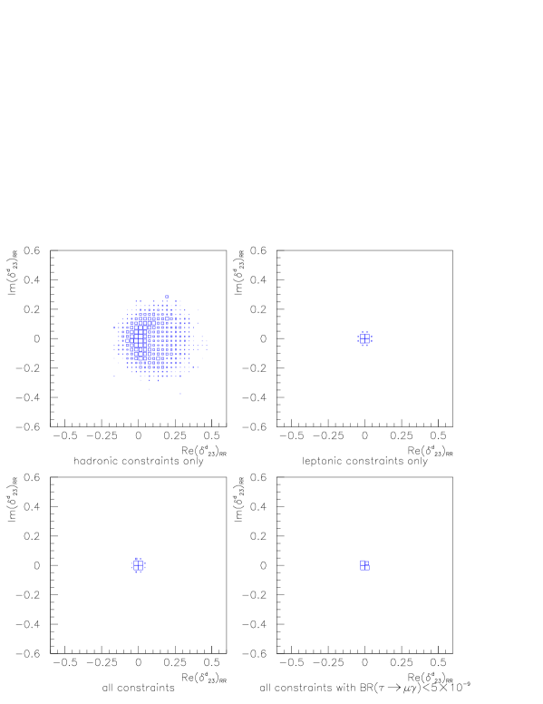
Figure 11: Allowed regions in the Re$(\delta^{d}_{23})_{RR}$–Im$(\delta^{d}_{23})_{RR}$ plane (top) and in the $S_{K\phi}$–Im$(\delta^{d}_{23})_{RR}$ plane (bottom). Constraints from $B\to X_{s}\gamma$, $BR(B\to X_{s}\ell^{+}\ell^{-})$, and the lower bound on $\Delta M_{s}$ have been used.

Thus, we can see that in a $SU(5)$ GUT model where SUSY-breaking terms have a supergravity origin, LFV constraints are indeed very relevant for $(\delta^{d}_{23})_{RR}$ and it is not possible to generate large effects on $A_{CP}(B\to\phi K_{s})$. Naturally we have to take into account that the leptonic bounds and their effects on hadronic MIs scale as $10/\tan\beta$ for different values of $\tan\beta$. However, even for $\tan\beta\leq 5$ the leptonic bounds would be very relevant on this MI.

Finally, we will also analyse the effects of leptonic constraints in the $12$ sector.

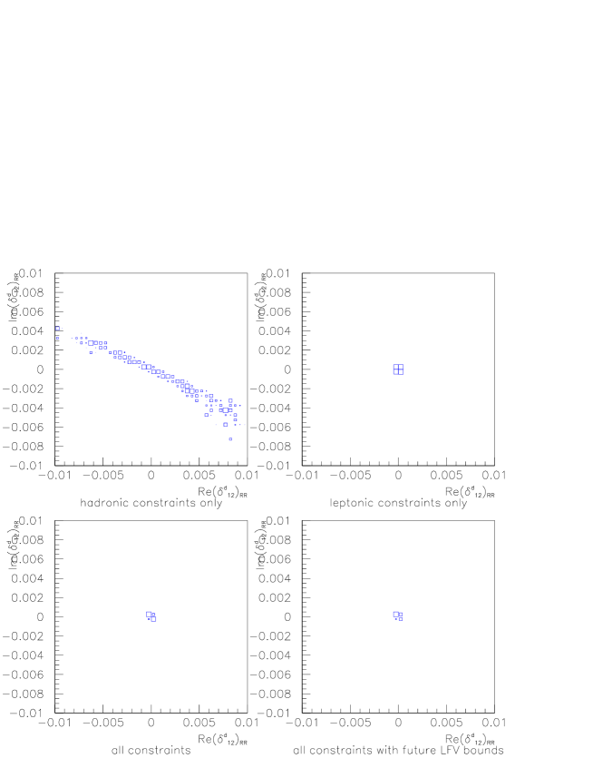
Figure 12: Allowed regions in the ${\rm Re}\left(\delta^{d}_{12}\right)_{\mbox{\scriptsize RR}}$– ${\rm Im}\left(\delta^{d}_{12}\right)_{\mbox{\scriptsize RR}}$ plane from hadronic and leptonic constraints. Upper left plot takes into account only hadronic bounds, upper right plot includes the present bound on the $\mu\to e\gamma$ decay, BR($\mu\to e,\gamma$)$<1.1~{}\times~{}10^{-11}$. The second row correspond to the projected bounds from the proposed LFV experiments, BR($\mu\to e,\gamma$)$<10^{-13}$ and BR($\mu\to e,\gamma$)$<10^{-14}$ respectively. We have to take into account that we use $\tan\beta=10$ and leptonic bounds scale as $10/\tan\beta$.

In Fig. 12 we present the allowed values of ${\rm Re}\left(\delta^{d}_{12}\right)_{\mbox{\scriptsize RR}}$ and ${\rm Im}\left(\delta^{d}_{12}\right)_{\mbox{\scriptsize RR}}$. The upper left plot corresponds to the values that satisfy the hadronic bounds, coming mainly from $\varepsilon_{K}=(2.284\pm 0.014)\times 10^{-3}$. The upper right plot takes also into account the present $\mu\to e\gamma$ bound, BR($\mu\to e,\gamma$)$<1.1~{}\times~{}10^{-11}$, and the plots in the second row correspond to projected bounds from the proposed experiments, BR($\mu\to e,\gamma$)$<10^{-13}$ and BR($\mu\to e,\gamma$)$<10^{-14}$ respectively. Now the GUT symmetry relates $\left(\delta^{d}_{12}\right)_{\mbox{\scriptsize RR}}$ to $\left(\delta^{l}_{12}\right)_{\mbox{\scriptsize LL}}$ and in this case leptonic bounds (already the present bounds) are very stringent and reduce the allowed values of $\left(\delta^{d}_{12}\right)_{\mbox{\scriptsize RR}}$ by more than one order of magnitude to a value $\left(\delta^{d}_{12}\right)_{\mbox{\scriptsize RR}}\leq 4\times 10^{-4}$ for $\tan\beta=10$.

In the case of $\left(\delta^{d}_{12}\right)_{\mbox{\scriptsize LL}}$ the $\mu\to e\gamma$ decay does not provide a bound to this MI due to the presence of cancellations between different contributions. We can only obtain a relatively mild bound, $\left(\delta_{12}^{l}\right)_{\mbox{\scriptsize RR}}\leq 0.09$ for $\tan\beta=10$, if we take into account $\mu\to eee$ and $\mu$–$e$ conversion in nuclei. After rescaling this bound by the factor ${\tilde{m}_{e^{c}}^{2}\over\tilde{m}_{d_{\rm L}}^{2}}$ the leptonic bound is still able to reduce the maximum values of ${\rm Re}\left(\delta^{d}_{12}\right)_{\mbox{\scriptsize LL}}$ and ${\rm Im}\left(\delta^{d}_{12}\right)_{\mbox{\scriptsize LL}}$ by a factor of 2, although the hadronic bound is still more constraining in a big part of the parameter space.

In summary, Supersymmetric Grand Unification predicts links between various leptonic and hadronic FCNC Observables. Though such relations can be constructed for any GUT group, we have concentrated on SU(5) and quantitatively studied the implications for the $23$ and $12$ sectors. In particular we have shown that the present limit on $BR(\tau\to\mu,\gamma)$ is sufficient to significantly constrain the observability of supersymmetry in CP violating B-decays.

3.5 SUSY-GUTs, SUSY-Seesaw and flavour blind Supersymmetry breaking

As discussed in the above, flavour violation can also be generated through renormalisation group running even if one starts with flavour-blind soft masses at the scale where supersymmetry is mediated to the visible sector. A classic example of this is the supersymmetric seesaw mechanism and the generation of lepton flavour violation at the weak scale.

The seesaw mechanism can be incorporated in the Minimal Supersymmetric Standard Model in a manner similar to what is done in the Standard Model by adding right-handed neutrino superfields to the MSSM superpotential:

$$W = h^{u}_{ij}Q_{i}u_{j}^{c}H_{2}+h^{d}_{ii}Q_{i}d_{i}^{c}H_{1}+h^{e}_{ii}L_{i}e^{c}_{i}H_{1}+h^{\nu}_{ij}L_{i}\nu^{c}_{j}H_{2}$$ (120)

$$+ M_{R_{ii}}\nu_{i}^{c}\nu_{i}^{c}+\mu H_{1}H_{2},$$

where we are in the basis of diagonal charged lepton, down quark and right-handed Majorana mass matrices. $M_{R}$ represents the (heavy) Majorana mass matrix for the right-handed neutrinos. Eq. (120) leads to the standard seesaw formula for the (light) neutrino mass matrix

$${\mathcal{M}}_{\nu}=-h^{\nu}M_{R}^{-1}h^{\nu~{}T}v_{2}^{2},$$ (121)

where $v_{2}$ is the vacuum expectation value (VEV) of the up-type Higgs field, $H_{2}$. Under suitable conditions on $h^{\nu}$ and $M_{R}$, the correct mass splittings and mixing angles in $\mathcal{M}_{\nu}$ can be obtained. Detailed analyses deriving these conditions are already present in the literature [151, 152, 153, 154, 155, 156, 157, 158].

Following the discussion in the previous section, we will assume that the mechanism that breaks supersymmetry and conveys it to the observable sector at the high scale $\sim M_{\rm P}$ is flavour-blind, as in the CMSSM (also called mSUGRA). However, this flavour blindness is not protected down to the weak scale [159] . The slepton mass matrices are no longer invariant under RG evolution from the super-large scale where supersymmetry is mediated to the visible sector down to the seesaw scale. The flavour violation present in the neutrino Dirac Yukawa couplings $h^{\nu}$ is now “felt” by the slepton mass matrices in the presence of heavy right-handed neutrinos [162, 163].

The weak-scale flavour violation so generated can be obtained by solving the RGEs for the slepton mass matrices from the high scale to the scale of the right-handed neutrinos. Below this scale, the running of the FV slepton mass terms is RG-invariant as the right-handed neutrinos decouple from the theory. For the purpose of illustration, a leading-log estimate can easily be obtained for these equations. Assuming the flavour blind mSUGRA specified by the high-scale parameters, $m_{0}$, the common scalar mass, $A_{0}$, the common trilinear coupling, and $M_{1/2}$, the universal gaugino mass, the flavour violating entries in these mass matrices at the weak scale are given as:

$$(\Delta^{l}_{ij})_{\rm LL}\approx-{3m_{0}^{2}+A_{0}^{2}\over 8\pi^{2}}\sum_{k}(h^{\nu}_{ik}h^{\nu*}_{jk})\ln{M_{X}\over M_{R_{k}}},$$ (122)

where $h^{\nu}$ are given in the basis of diagonal charged lepton masses and diagonal Majorana right-handed neutrino mass matrix $M_{R}$, and $M_{X}$ is the scale at which soft terms appear in the Lagrangian. Given this, the branching ratios for LFV rare decays $l_{j}\to l_{i},\gamma$ can be roughly estimated using

$$\mbox{BR}(l_{j}\to l_{i}\gamma)\approx\frac{\displaystyle{\alpha^{3}~{}~{}|\delta^{l}_{ij}|^{2}}}{\displaystyle{G_{F}^{2}~{}m^{4}_{\rm SUSY}}}\tan^{2}\beta.$$ (123)

From above it is obvious that the amount of lepton flavour violation generated by the SUSY seesaw at the weak scale crucially depends on the flavour structure of $h^{\nu}$ and $M_{R}$, the “new” sources of flavour violation not present in the MSSM, Eq. (120). If either the neutrino Yukawa couplings or the flavour mixings present in $h^{\nu}$ are very tiny, the strength of LFV will be significantly reduced. Further, if the right-handed neutrino masses were heavier than the supersymmetry breaking scale (as in GMSB models) they would decouple from the theory before the SUSY soft breaking matrices enter into play and hence these effects would vanish.

3.6 Seesaw in GUTs: SO(10) and LFV

A simple analysis of the fermion mass matrices in the $SO(10)$ model, as detailed in the Eq. (72) leads us to the following result: At least one of the Yukawa couplings in $h^{\nu}~{}=~{}v_{u}^{-1}~{}M^{\nu}_{LR}$ has to be as large as the top Yukawa coupling [149]. This result holds true in general, independently of the choice of the Higgses responsible for the masses in Eqs. (71), (72), provided that no accidental fine-tuned cancellations of the different contributions in Eq. (72) are present. If contributions from the 10’s solely dominate, $h^{\nu}$ and $h^{u}$ would be equal. If this occurs for the 126’s, then $h^{\nu}=-3~{}h^{u}$ [165]. In case both of them have dominant entries, barring a rather precisely fine-tuned cancellation between $M^{5}_{10}$ and $M^{5}_{126}$ in Eq. (72), we expect at least one large entry to be present in $h^{\nu}$. A dominant antisymmetric contribution to top quark mass due to the 120 Higgs is phenomenologically excluded, since it would lead to at least a pair of heavy degenerate up quarks.

Apart from sharing the property that at least one eigenvalue of both $M^{u}$ and $M^{\nu}_{LR}$ has to be large, for the rest it is clear from Eqs. (71) and (72) that these two matrices are not aligned in general, and hence we may expect different mixing angles appearing from their diagonalisation. This freedom is removed if one sticks to particularly simple choices of the Higgses responsible for up quark and neutrino masses. A couple of remarks are in order here. Firstly, note that in general there can be an additional contribution, Eq. (75), to the light neutrino mass matrix, independent of the canonical seesaw mechanism. Taking into consideration also this contribution leads to the so-called Type-II seesaw formula [166, 167]. Secondly, the correlation between neutrino Dirac Yukawa coupling and the top Yukawa is in general independent of the type of seesaw mechanism, and thus holds true irrespective of the light-neutrino mass structure.

Therefore, we see that the $SO(10)$ model with only two ten-plets would inevitably lead to small mixing in $h^{\nu}$. In fact, with two Higgs fields in symmetric representations, giving masses to the up-sector and the down-sector separately, it would be difficult to avoid the small CKM-like mixing in $h^{\nu}$. We will call this case the CKM case. From here, the following mass relations hold between the quark and leptonic mass matrices at the GUT scale:

$$h^{u}=h^{\nu}\;\;\;;\;\;\;h^{d}=h^{e}.$$ (124)

In the basis where charged lepton masses are diagonal, we have

$$h^{\nu}=V_{\rm CKM}^{T}~{}h^{u}_{Diag}~{}V_{\rm CKM}.$$ (125)

The large couplings in $h^{\nu}\sim{\mathcal{O}}(h_{t})$ induce significant off-diagonal entries in $m_{\tilde{L}}^{2}$ through the RG evolution between $M_{\rm GUT}$ and the scale of the right-handed Majorana neutrinos , $M_{R_{i}}$. The induced off-diagonal entries relevant to $l_{j}\rightarrow l_{i},\gamma$ are of the order of:

$$(m_{\tilde{L}}^{2})_{21} \approx -{3m_{0}^{2}+A_{0}^{2}\over 8\pi^{2}}~{}h_{t}^{2}V_{td}V_{ts}\ln{M_{\rm GUT}\over M_{R_{3}}}+\mathcal{O}(h_{c}^{2}),$$ (126)

$$(m_{\tilde{L}}^{2})_{32} \approx -{3m_{0}^{2}+A_{0}^{2}\over 8\pi^{2}}~{}h_{t}^{2}V_{tb}V_{ts}\ln{M_{\rm GUT}\over M_{R_{3}}}+\mathcal{O}(h_{c}^{2}),$$ (127)

$$(m_{\tilde{L}}^{2})_{31} \approx -{3m_{0}^{2}+A_{0}^{2}\over 8\pi^{2}}~{}h_{t}^{2}V_{tb}V_{td}\ln{M_{\rm GUT}\over M_{R_{3}}}+\mathcal{O}(h_{c}^{2}).$$ (128)

In these expressions, the CKM angles are small but one would expect the presence of the large top Yukawa coupling to compensate such a suppression. The required right-handed neutrino Majorana mass matrix, consistent with both the observed low energy neutrino masses and mixings as well as with CKM-like mixings in $h^{\nu}$ is easily determined from the seesaw formula defined at the scale of right-handed neutrinos .

The Br($l_{i}\to l_{j}\gamma$) are now predictable in this case. Considering mSUGRA boundary conditions and taking $\tan\beta=40$, we obtain that reaching a sensitivity of $10^{-14}$ for BR$(\mu\to e\gamma)$ would allow us to probe the SUSY spectrum completely up to $M_{1/2}=300$ GeV (notice that this corresponds to gluino and squark masses of order 750 GeV) and would still probe large regions of the parameter space up to $M_{1/2}=700$ GeV. Thus, in summary, though the present limits on BR($\mu\to e,\gamma$) would not induce any significant constraints on the supersymmetry-breaking parameter space, an improvement in the limit to $\sim{\mathcal{O}}(10^{-14})$, as foreseen, would start imposing non-trivial constraints especially for the large $\tan\beta$ region.

To obtain mixing angles larger than CKM angles, asymmetric mass matrices have to be considered. In general, it is sufficient to introduce asymmetric textures either in the up-sector or in the down-sector. In the present case, we assume that the down-sector couples to a combination of Higgs representations (symmetric and antisymmetric) $\Phi$, leading to an asymmetric mass matrix in the basis where the up-sector is diagonal. As we will see below, this would also require that the right-handed Majorana mass matrix be diagonal in this basis. We have :

$$W_{SO(10)}={1\over 2}~{}h^{u,\nu}_{ii}~{}{\bf 16_{i}}~{}{\bf 16_{i}}{\bf 10^{u}}+{1\over 2}~{}h^{d,e}_{ij}~{}{\bf 16_{i}}~{}{\bf 16_{j}}\Phi\\ +{1\over 2}~{}h^{R}_{ii}~{}{\bf 16_{i}}~{}{\bf 16_{i}}{\bf 126}~{},$$

where the 126, as before, generates only the right-handed neutrino mass matrix. To study the consequences of these assumptions, we see that at the level of $SU(5)$, we have

$$W_{SU(5)}={1\over 2}~{}h^{u}_{ii}~{}{\bf 10_{i}}~{}{\bf 10_{i}}~{}{\bf 5_{u}}+h^{\nu}_{ii}~{}{\bf\bar{5}_{i}}~{}{\bf 1_{i}}~{}{\bf 5_{u}}\\ +h^{d}_{ij}~{}{\bf 10_{i}}~{}{\bf\bar{5}_{j}}~{}{\bf\bar{5}_{d}}+{1\over 2}~{}M^{R}_{ii}~{}{\bf 1_{i}}{\bf 1_{i}},$$

where we have decomposed the ${\bf 16}$ into ${\bf 10}+{\bf\bar{5}}+{\bf 1}$ and ${\bf 5_{u}}$ and ${\bf\bar{5}_{d}}$ are components of ${\bf 10_{u}}$ and $\Phi$ respectively. To have large mixing $\sim~{}U_{\rm PMNS}$ in $h^{\nu}$ we see that the asymmetric matrix $h^{d}$ should now give rise to both the CKM mixing as well as PMNS mixing. This is possible if

$$V_{\rm CKM}^{T}~{}h^{d}~{}U_{\rm PMNS}^{T}=h^{d}_{Diag}.$$ (129)

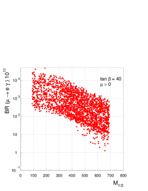
Figure 13: The scatter plots of branching ratios of $\mu\to e,\gamma$ decays as a function of $M_{1/2}$ are shown for the (maximal) PMNS case for tan $\beta$ = 40. The results do not alter significantly with the change of sign($\mu$).

Therefore the ${\bf 10}$ that contains the left-handed down-quarks would be rotated by the CKM matrix whereas the ${\bf\bar{5}}$ that contains the left-handed charged leptons would be rotated by the $U_{\rm PMNS}$ matrix to go into their respective mass bases [173, 174, 175, 115]. Thus we have, in analogy with the previous subsection, the following relations in the basis where charged leptons and down quarks are diagonal:

$$h^{u} = V_{\rm CKM}~{}h^{u}_{Diag}~{}V_{\rm CKM}^{T}~{},$$ (130)

$$h^{\nu} = U_{\rm PMNS}~{}h^{u}_{Diag}.$$ (131)

Using the seesaw formula of Eqs. (121) and (131), we have

$$M_{R}=Diag\{{m_{u}^{2}\over m_{\nu_{1}}},~{}{m_{c}^{2}\over m_{\nu_{2}}},~{}{m_{t}^{2}\over m_{\nu_{3}}}\}.$$ (132)

We now turn our attention to lepton flavour violation in this case. The branching ratio, BR($\mu\rightarrow e,\gamma)$ would now depend on

$$[h^{\nu}h^{\nu~{}T}]_{21}=h_{t}^{2}~{}U_{\mu 3}~{}U_{e3}+h_{c}^{2}~{}U_{\mu 2}~{}U_{e2}+\mathcal{O}(h_{u}^{2}).$$ (133)

It is clear from the above that in contrast to the CKM case, the dominant contribution to the off-diagonal entries depends on the unknown magnitude of the element $U_{e3}$ [176]. If $U_{e3}$ is very close to its present limit $\sim~{}0.2$ [177], the first term on the RHS of the Eq. (133) would dominate. Moreover, this would lead to large contributions to the off-diagonal entries in the slepton masses with $U_{\mu 3}$ of ${\mathcal{O}}(1)$. From Eq. (122) we have

$$(m_{\tilde{L}}^{2})_{21}\approx-{3m_{0}^{2}+A_{0}^{2}\over 8\pi^{2}}~{}h_{t}^{2}U_{e3}U_{\mu 3}\ln{M_{\rm GUT}\over M_{R_{3}}}+\mathcal{O}(h_{c}^{2}).$$ (134)

This contribution is larger than the CKM case by a factor of $(U_{\mu 3}U_{e3})/(V_{td}V_{ts})\sim 140$. From Eq. (123) we see that it would mean about a factor $10^{4}$ times larger than the CKM case in BR($\mu\rightarrow e,\gamma)$. In case $U_{e3}$ is very small, i.e either zero or $\stackrel{{\scriptstyle\scriptstyle<}}{{\scriptstyle\sim}}~{}(h_{c}^{2}/h_{t}^{2})~{}U_{e2}~{}\sim 4\times 10^{-5}$, the second term $\propto~{}h_{c}^{2}$ in Eq. (133) would dominate. However the off-diagonal contribution in slepton masses, now being proportional to charm Yukawa could be much smaller, even smaller than the CKM contribution by a factor

$${h_{c}^{2}~{}U_{\mu 2}~{}U_{e2}\over h_{t}^{2}~{}V_{td}~{}V_{ts}}\sim 7\times 10^{-2}.$$ (135)

If $U_{e3}$ is close to its present limit, the current bound on R($\mu\rightarrow e,\gamma$) would already be sufficient to produce stringent limits on the SUSY mass spectrum. Similar $U_{e3}$ dependence can be expected in the $\tau\to e$ transitions where the off-diagonal entries are given by :

$$(m_{\tilde{L}}^{2})_{31}\approx-{3m_{0}^{2}+A_{0}^{2}\over 8\pi^{2}}~{}h_{t}^{2}U_{e3}U_{\tau 3}\ln{M_{\rm GUT}\over M_{R_{3}}}+\mathcal{O}(h_{c}^{2}).$$ (136)

The $\tau\to\mu$ transitions are instead $U_{e3}$-independent probes of SUSY, whose importance was first pointed out in Ref. [178]. The off-diagonal entry in this case is given by :

$$(m_{\tilde{L}}^{2})_{32}\approx-{3m_{0}^{2}+A_{0}^{2}\over 8\pi^{2}}~{}h_{t}^{2}U_{\mu 3}U_{\tau 3}\ln{M_{\rm GUT}\over M_{R_{3}}}\mathcal{O}(h_{c}^{2}).$$ (137)

In the PMNS scenario, Fig. 3 shows the plot for BR($\mu\rightarrow e,\gamma$) for tan $\beta$ = 40. In this plot, the value of $U_{e3}$ chosen is very close to the present experimental upper limit [177]. As long as $U_{e3}\stackrel{{\scriptstyle\scriptstyle>}}{{\scriptstyle\sim}}4\times 10^{-5}$, the plots scale as $U_{e3}^{2}$, while for $U_{e3}\stackrel{{\scriptstyle\scriptstyle<}}{{\scriptstyle\sim}}4\times 10^{-5}$ the term proportional to $m_{c}^{2}$ in Eq. (134) starts dominating; the result is then insensitive to the choice of $U_{e3}$. For instance, a value of $U_{e3}=0.01$ would reduce the BR by a factor of 225 and still a significant amount of the parameter space for $\tan\beta=40$ would be excluded. We further find that with the present limit on BR($\mu\rightarrow e,\gamma$), all the parameter space would be completely excluded up to $M_{1/2}=300$ GeV for $U_{e3}=0.15$, for any vale of $\tan\beta$ (not shown in the figure).

In the $\tau\to\mu\gamma$ decay the situation is similarly constrained. For $\tan\beta=2$, the present bound of $3\times 10^{-7}$ starts probing the parameter space up to $M_{1/2}\leq 150$ GeV. The main difference is that this does not depend on the value of $U_{e3}$, and therefore it is already a very important constraint on the parameter space of the model. In fact, for large $\tan\beta=40$, as shown in Fig. 4, reaching the expected limit of $1\times 10^{-8}$ would be able to rule out completely this scenario up to gaugino masses of $400$ GeV, and only a small portion of the parameter space with heavier gauginos would survive. In the limit $U_{e3}=0$, this decay mode would provide a constraint on the model stronger than $\mu\to e,\gamma$, which would now be suppressed as it would contain only contributions proportional to $h_{c}^{2}$, as shown in Eq. (134).

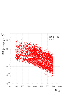
Figure 14: The scatter plots of branching ratios of $\tau\to\mu,\gamma$ decays as a function of $M_{1/2}$ are shown for the (maximal) PMNS case for n the PMNS scenario, Fig. 3 shows the plot for BR($\mu$ tan $\beta$ = 40. The results do not alter significantly with the change of sign($\mu$).

In summary, in the PMNS/maximal mixing case, even the present limits from BR($\mu\to e,\gamma$ ) can rule out large portions of the supersymmetry-breaking parameter space if $U_{e3}$ is either close to its present limit or within an order of magnitude of it (as the planned experiments might find out soon [179]). These limits are more severe for large $\tan\beta$. In the extreme situation of $U_{e3}$ being zero or very small $\sim{\mathcal{O}}(10^{-4}-10^{-5})$, BR($\tau\to\mu\gamma$) will start playing an important role with its present constraints already disallowing large regions of the parameter space at large $\tan\beta$. While the above example concentrated on the hierarchical light neutrinos, similar ‘benchmark’ mixing scenarios have been explored in great detail, for degenerate spectra of light neutrinos, by Ref. [180], taking also in to consideration running between the Planck scale and the GUT scale.

The above analysis has been restricted to one of the breaking chains of SO(10), namely the one which directly breaks in to MSSM. As depicted in Fig. 7, there could be other breaking chains too. For example, let us consider the SU(5) breaking chain of SO(10) discussed in Fig. 7. The various energy scales involved in this model can be neatly summarised as in figure 15. In this case, there could be addional sources of LFV other than the ones appearing in the direct breaking chain.

Figure 15: Schematic picture of the energy scales involved in the model.

These sources are due to the result of $SU(5)$ running between the scales $M_{SU(5)}$ and the $SO(10)$ scale $M_{SO(10)}$. As we have seen several times already in SU(5) the right handed leptonic singlets sit in the same multiplet as the quark doublets (left handed) and up-type singlets ($q,u,e^{c}$). This would have implications for the ‘right handed mixing’ ($\Delta_{RR}^{l}$) as this would get generated through RG evolution, due to the couplings of the up-type quarks carrying the CKM information [181]. This new contribution adds up to the $\Delta_{LL}^{l}$ contributions to LFV already present due to the seesaw effect. An analysis similar to the previous one could now be repeated for this breaking chain and it can be seen that these additional contributions become important in some regions of the parameter space[182].

Finally, let us in passing touch up on two related topics which are outside the realm of the present lecture series but are however quite important in their own right. One of them relates the visibility of supersymmetry at Large Hadron Collider/ International Linear Collider with the indirect evidence for SUSY in flavour experiments or the dark matter experiments. This is an important question, in particular, in simple models based on Grand Unification where the inter-correlations between the various SUSY stratergies are quite interesting and could play an important role in ”solving” the inverse LHC problem. While, in general, direct searches at colliders like LHC/ILC are superior in comparison with indirect search strategies at flavour machines and dark matter experiments, there could be regions in the parameter space where the flavour machines can strike back. For example, in simple GUTs based on SUSY $SO(10)$ and in the case of the focus point region for viable dark matter, the sensistivity in flavour experiments is far greater than in direct searches at LHC[183]. On an independent note, irrespective of flavour violation, SUSY-GUTs can modify the pattern of dark matter parameter space itselves as has been pointed out in [184], [185]. So, dark matter and flavour violation can both play an important and complementary role in unravelling the structure of SUSY-GUTs.

Finally, a second interesting aspect we have not addressed in the present lectures is the role of CP violation in the generation of the flavour asymmetry of the universe in the context of SUSY-GUTs. CP violation can play an important role for leptogenesis which can explain the observed matter-anti-matter asymmetry. While in the simplest SO(10) models, which we have discussed above, it might be very difficult to achieve viable leptogenesis[186], there have been simple solutions proposed which might make it achievable [187].

CONCLUSIONS

The ideas of the Grand Unification and Supersymmetry are closely connected and represent the main avenue to explore in the search of physics beyond the Standard Model. In these lectures we have presented the reasons that make us believe in the existence of new physics beyond the SM. We have presented the (non-supersymmetric) Grand Unification idea and analysed its achievements and failures. Supersymmetric grand unification was shown to cure some of these problems and make the construction of “realistic” models possible. The phenomenology of low-energy supersymmetry has been discussed in the second part of these lectures with special emphasis on the SUSY flavour and CP problems. We have seen that, quite generally, SUSY extensions of the SM lead to the presence of a host of new flavour and CP violation parameters. The solution of the “SUSY flavour problem” and the “SUSY CP problem” are intimately linked. However, there is an “intrinsic” CP problem in SUSY which goes beyond the flavour issue and requires a deeper comprehension of the link between CP violation and breaking of SUSY. We tried to emphasise that the these two problems have not only a dark and worrying side, but also they provide promising tools to obtain indirect SUSY hints. We have also seen that the presence of a grand unified symmetry and/or new particles, like right-handed neutrinos, at super-large scales has observable consequences in the structure of soft masses at the electroweak scale. Thus the discovery of low energy SUSY at the LHC or low energy FCNC experiments and the measurement of the SUSY spectrum may provide a fundamental clue for the assessment of SUSY GUTs and SUSY seesaw in nature.

References

- [1] Y. Nir, (2005), hep-ph/0510413, Lectures at Les Houches summer school: Physics beyond the SM.
- [2] A. Y. Smirnov, Neutrino physics, Lectures at Les Houches summer school: Physics beyond the SM, 2005.
- [3] P. Binetruy, Astroparticle physics and cosmology, Lectures at Les Houches summer school: Physics beyond the SM, 2005.
- [4] J. R. Ellis and D. V. Nanopoulos, Phys. Lett. B110, 44 (1982).
- [5] R. Barbieri and R. Gatto, Phys. Lett. B110, 211 (1982).
- [6] M. J. Duncan and J. Trampetic, Phys. Lett. B134, 439 (1984).
- [7] J. M. Gerard, W. Grimus, A. Raychaudhuri, and G. Zoupanos, Phys. Lett. B140, 349 (1984).
- [8] J. M. Gerard, W. Grimus, A. Masiero, D. V. Nanopoulos, and A. Raychaudhuri, Phys. Lett. B141, 79 (1984).
- [9] P. Langacker and B. Sathiapalan, Phys. Lett. B144, 401 (1984).
- [10] J. M. Gerard, W. Grimus, A. Masiero, D. V. Nanopoulos, and A. Raychaudhuri, Nucl. Phys. B253, 93 (1985).
- [11] R. Barbieri, S. Ferrara, and C. A. Savoy, Phys. Lett. B119, 343 (1982).
- [12] A. H. Chamseddine, R. Arnowitt, and P. Nath, Phys. Rev. Lett. 49, 970 (1982).
- [13] H. P. Nilles, Phys. Rept. 110, 1 (1984).
- [14] H. E. Haber and G. L. Kane, Phys. Rept. 117, 75 (1985).
- [15] G. G. Ross, Reading, Usa: Benjamin/cummings ( 1984) 497 P. ( Frontiers In Physics, 60).
- [16] H. E. Haber, (1993), hep-ph/9306207.
- [17] S. P. Martin, (1997), hep-ph/9709356.
- [18] G. F. Giudice and R. Rattazzi, Phys. Rept. 322, 419 (1999), hep-ph/9801271.
- [19] R. N. Mohapatra, Adv. Ser. Direct. High Energy Phys. 3, 436 (1989).
- [20] Y. Grossman, Y. Nir, and R. Rattazzi, Adv. Ser. Direct. High Energy Phys. 15, 755 (1998), hep-ph/9701231.
- [21] M. Misiak, S. Pokorski, and J. Rosiek, Adv. Ser. Direct. High Energy Phys. 15, 795 (1998), hep-ph/9703442.
- [22] A. Masiero and O. Vives, Ann. Rev. Nucl. Part. Sci. 51, 161 (2001), hep-ph/0104027.
- [23] A. Masiero and O. Vives, New J. Phys. 4, 4 (2002).
- [24] J. C. Pati and A. Salam, Phys. Rev. D10, 275 (1974).
- [25] H. Georgi and S. L. Glashow, Phys. Rev. Lett. 32, 438 (1974).
- [26] H. Fritzsch and P. Minkowski, Ann. Phys. 93, 193 (1975).
- [27] H. Georgi and D. V. Nanopoulos, Nucl. Phys. B155, 52 (1979).
- [28] H. Georgi, H. R. Quinn, and S. Weinberg, Phys. Rev. Lett. 33, 451 (1974).
- [29] I. Antoniadis, C. Kounnas, and C. Roiesnel, Nucl. Phys. B198, 317 (1982).
- [30] P. Langacker, Phys. Rept. 72, 185 (1981).
- [31] D. V. Nanopoulos and D. A. Ross, Nucl. Phys. B157, 273 (1979).
- [32] D. V. Nanopoulos and D. A. Ross, Phys. Lett. B108, 351 (1982).
- [33] H. Georgi and C. Jarlskog, Phys. Lett. B86, 297 (1979).
- [34] A. J. Buras, J. R. Ellis, M. K. Gaillard, and D. V. Nanopoulos, Nucl. Phys. B135, 66 (1978).
- [35] S. Weinberg, Phys. Rev. Lett. 43, 1566 (1979).
- [36] S. Weinberg, Phys. Rev. D22, 1694 (1980).
- [37] F. Wilczek and A. Zee, Phys. Rev. Lett. 43, 1571 (1979).
- [38] H. A. Weldon and A. Zee, Nucl. Phys. B173, 269 (1980).
- [39] W. J. Marciano, Presented at 4th Workshop on Grand Unification, Philadelphia, Pa., Apr 21-23, 1983.
- [40] M. Drees, (1996), hep-ph/9611409.
- [41] L. Girardello and M. T. Grisaru, Nucl. Phys. B194, 65 (1982).
- [42] M. Carena and C. Wagner, Higgs physics and supersymmetry phenomenology, Lectures at Les Houches summer school: Physics beyond the SM, 2005.
- [43] S. Dimopoulos, S. Raby, and F. Wilczek, Phys. Rev. D24, 1681 (1981).
- [44] W. J. Marciano and G. Senjanovic, Phys. Rev. D25, 3092 (1982).
- [45] U. Amaldi, W. de Boer, P. H. Frampton, H. Furstenau, and J. T. Liu, Phys. Lett. B281, 374 (1992).
- [46] R. N. Mohapatra, (1999), hep-ph/9911272.
- [47] A. Masiero, D. V. Nanopoulos, K. Tamvakis, and T. Yanagida, Phys. Lett. B115, 380 (1982).
- [48] R. Arnowitt, A. H. Chamseddine, and P. Nath, Phys. Lett. B156, 215 (1985).
- [49] P. Nath, A. H. Chamseddine, and R. Arnowitt, Phys. Rev. D32, 2348 (1985).
- [50] G. Altarelli, F. Feruglio, and I. Masina, JHEP 11, 040 (2000), hep-ph/0007254.
- [51] G. F. Giudice and A. Masiero, Phys. Lett. B206, 480 (1988).
- [52] P. Minkowski, Phys. Lett. B67, 421 (1977).
- [53] T. Yanagida, In Proceedings of the Workshop on the Baryon Number of the Universe and Unified Theories, Tsukuba, Japan, 13-14 Feb 1979.
- [54] M. Gell-Mann, P. Ramond, and R. Slansky, Print-80-0576 (CERN).
- [55] R. N. Mohapatra and G. Senjanovic, Phys. Rev. Lett. 44, 912 (1980).
- [56] J. Schechter and J. W. F. Valle, Phys. Rev. D22, 2227 (1980).
- [57] R. Barbieri, D. V. Nanopoulos, G. Morchio, and F. Strocchi, Phys. Lett. B90, 91 (1980).
- [58] P. Nath and R. M. Syed, Phys. Lett. B506, 68 (2001), hep-ph/0103165.
- [59] J. Wess and J. Bagger, Princeton, USA: Univ. Pr. (1992) 259 p.
- [60] G. R. Farrar and P. Fayet, Phys. Lett. B76, 575 (1978).
- [61] H. K. Dreiner, (1997), hep-ph/9707435.
- [62] H. E. Haber, Nucl. Phys. Proc. Suppl. 62, 469 (1998), hep-ph/9709450.
- [63] S. Dimopoulos and S. Thomas, Nucl. Phys. B465, 23 (1996), hep-ph/9510220.
- [64] A. Santamaria, Phys. Lett. B305, 90 (1993), hep-ph/9302301.
- [65] F. J. Botella, M. Nebot, and O. Vives, JHEP 01, 106 (2006), hep-ph/0407349.
- [66] V. S. Kaplunovsky and J. Louis, Phys. Lett. B306, 269 (1993), hep-th/9303040.
- [67] A. Brignole, L. E. Ibanez, and C. Munoz, Nucl. Phys. B422, 125 (1994), hep-ph/9308271.
- [68] L. E. Ibanez and G. G. Ross, (1992), hep-ph/9204201.
- [69] L. J. Hall, V. A. Kostelecky, and S. Raby, Nucl. Phys. B267, 415 (1986).
- [70] F. Gabbiani and A. Masiero, Nucl. Phys. B322, 235 (1989).
- [71] J. S. Hagelin, S. Kelley, and T. Tanaka, Nucl. Phys. B415, 293 (1994).
- [72] F. Gabbiani, E. Gabrielli, A. Masiero, and L. Silvestrini, Nucl. Phys. B477, 321 (1996), hep-ph/9604387.
- [73] J. R. Ellis, S. Ferrara, and D. V. Nanopoulos, Phys. Lett. B114, 231 (1982).
- [74] W. Buchmuller and D. Wyler, Phys. Lett. B121, 321 (1983).
- [75] J. Polchinski and M. B. Wise, Phys. Lett. B125, 393 (1983).
- [76] E. Franco and M. L. Mangano, Phys. Lett. B135, 445 (1984).
- [77] M. Dugan, B. Grinstein, and L. J. Hall, Nucl. Phys. B255, 413 (1985).
- [78] W. Fischler, S. Paban, and S. Thomas, Phys. Lett. B289, 373 (1992), hep-ph/9205233.
- [79] P. G. Harris et al., Phys. Rev. Lett. 82, 904 (1999).
- [80] B. C. Regan, E. D. Commins, C. J. Schmidt, and D. DeMille, Phys. Rev. Lett. 88, 071805 (2002).
- [81] A. J. Buras, A. Romanino, and L. Silvestrini, Nucl. Phys. B520, 3 (1998), hep-ph/9712398.
- [82] J. Hisano and D. Nomura, Phys. Rev. D59, 116005 (1999), hep-ph/9810479.
- [83] L. Clavelli, T. Gajdosik, and W. Majerotto, Phys. Lett. B494, 287 (2000), hep-ph/0007342.
- [84] S. Abel, S. Khalil, and O. Lebedev, Nucl. Phys. B606, 151 (2001), hep-ph/0103320.
- [85] V. D. Barger et al., Phys. Rev. D64, 056007 (2001), hep-ph/0101106.
- [86] S. Weinberg, Phys. Rev. Lett. 63, 2333 (1989).
- [87] T. Ibrahim and P. Nath, Phys. Lett. B418, 98 (1998), hep-ph/9707409.
- [88] T. Ibrahim and P. Nath, Phys. Rev. D57, 478 (1998), hep-ph/9708456.
- [89] D. Chang, W.-Y. Keung, and A. Pilaftsis, Phys. Rev. Lett. 82, 900 (1999), hep-ph/9811202.
- [90] M. Pospelov and A. Ritz, Phys. Rev. D63, 073015 (2001), hep-ph/0010037.
- [91] T. Ibrahim and P. Nath, Phys. Rev. D58, 111301 (1998), hep-ph/9807501.
- [92] M. Brhlik, G. J. Good, and G. L. Kane, Phys. Rev. D59, 115004 (1999), hep-ph/9810457.
- [93] A. Bartl, T. Gajdosik, W. Porod, P. Stockinger, and H. Stremnitzer, Phys. Rev. D60, 073003 (1999), hep-ph/9903402.
- [94] M. Brhlik, L. L. Everett, G. L. Kane, and J. Lykken, Phys. Rev. Lett. 83, 2124 (1999), hep-ph/9905215.
- [95] M. Brhlik, L. L. Everett, G. L. Kane, and J. Lykken, Phys. Rev. D62, 035005 (2000), hep-ph/9908326.
- [96] T. Ibrahim and P. Nath, Phys. Rev. D61, 093004 (2000), hep-ph/9910553.
- [97] A. Bartl et al., Phys. Rev. D64, 076009 (2001), hep-ph/0103324.
- [98] S. Abel, S. Khalil, and O. Lebedev, Phys. Rev. Lett. 86, 5850 (2001), hep-ph/0103031.
- [99] O. Lebedev, K. A. Olive, M. Pospelov, and A. Ritz, Phys. Rev. D70, 016003 (2004), hep-ph/0402023.
- [100] M. Ciuchini et al., JHEP 10, 008 (1998), hep-ph/9808328.
- [101] G. G. Ross, L. Velasco-Sevilla, and O. Vives, Nucl. Phys. B692, 50 (2004), hep-ph/0401064.
- [102] K. S. Babu, J. C. Pati, and P. Rastogi, (2004), hep-ph/0410200.
- [103] K. S. Babu, J. C. Pati, and P. Rastogi, Phys. Lett. B621, 160 (2005), hep-ph/0502152.
- [104] A. Masiero and O. Vives, Phys. Rev. Lett. 86, 26 (2001), hep-ph/0007320.
- [105] A. Masiero, M. Piai, and O. Vives, Phys. Rev. D64, 055008 (2001), hep-ph/0012096.
- [106] S. Bertolini, F. Borzumati, A. Masiero, and G. Ridolfi, Nucl. Phys. B353, 591 (1991).
- [107] M. Ciuchini, E. Franco, G. Martinelli, A. Masiero, and L. Silvestrini, Phys. Rev. Lett. 79, 978 (1997), hep-ph/9704274.
- [108] D. Becirevic et al., Nucl. Phys. B634, 105 (2002), hep-ph/0112303.
- [109] BABAR, B. Aubert et al., Phys. Rev. Lett. 89, 201802 (2002), hep-ex/0207042.
- [110] Belle, K. Abe et al., Phys. Rev. Lett. 87, 091802 (2001), hep-ex/0107061.
- [111] Belle, K. Abe et al., (2003), hep-ex/0308036.
- [112] CDF, T. Affolder et al., Phys. Rev. D61, 072005 (2000), hep-ex/9909003.
- [113] E. Lunghi and D. Wyler, Phys. Lett. B521, 320 (2001), hep-ph/0109149.
- [114] T. Goto, Y. Okada, Y. Shimizu, T. Shindou, and M. Tanaka, Phys. Rev. D66, 035009 (2002), hep-ph/0204081.
- [115] D. Chang, A. Masiero, and H. Murayama, Phys. Rev. D67, 075013 (2003), hep-ph/0205111.
- [116] S. Khalil and E. Kou, Phys. Rev. D67, 055009 (2003), hep-ph/0212023.
- [117] R. Harnik, D. T. Larson, H. Murayama, and A. Pierce, Phys. Rev. D69, 094024 (2004), hep-ph/0212180.
- [118] M. Ciuchini, E. Franco, A. Masiero, and L. Silvestrini, Phys. Rev. D67, 075016 (2003), hep-ph/0212397.
- [119] S. Baek, Phys. Rev. D67, 096004 (2003), hep-ph/0301269.
- [120] K. Agashe and C. D. Carone, Phys. Rev. D68, 035017 (2003), hep-ph/0304229.
- [121] G. L. Kane et al., Phys. Rev. Lett. 90, 141803 (2003), hep-ph/0304239.
- [122] S. Mishima and A. I. Sanda, Phys. Rev. D69, 054005 (2004), hep-ph/0311068.
- [123] M. Endo, M. Kakizaki, and M. Yamaguchi, Phys. Lett. B594, 205 (2004), hep-ph/0403260.
- [124] M. Endo, S. Mishima, and M. Yamaguchi, Phys. Lett. B609, 95 (2005), hep-ph/0409245.
- [125] BABAR, B. Aubert et al., (2002), hep-ex/0207070.
- [126] Belle, K. Abe et al., Phys. Rev. Lett. 91, 261602 (2003), hep-ex/0308035.
- [127] E. Gabrielli and G. F. Giudice, Nucl. Phys. B433, 3 (1995), hep-lat/9407029.
- [128] A. Masiero and H. Murayama, Phys. Rev. Lett. 83, 907 (1999), hep-ph/9903363.
- [129] G. Eyal, A. Masiero, Y. Nir, and L. Silvestrini, JHEP 11, 032 (1999), hep-ph/9908382.
- [130] R. Barbieri, R. Contino, and A. Strumia, Nucl. Phys. B578, 153 (2000), hep-ph/9908255.
- [131] K. S. Babu, B. Dutta, and R. N. Mohapatra, Phys. Rev. D61, 091701 (2000), hep-ph/9905464.
- [132] S. Khalil, T. Kobayashi, and O. Vives, Nucl. Phys. B580, 275 (2000), hep-ph/0003086.
- [133] A. J. Buras, P. Gambino, M. Gorbahn, S. Jager, and L. Silvestrini, Nucl. Phys. B592, 55 (2001), hep-ph/0007313.
- [134] NA31, G. D. Barr et al., Phys. Lett. B317, 233 (1993).
- [135] KTeV, A. Alavi-Harati et al., Phys. Rev. Lett. 83, 22 (1999), hep-ex/9905060.
- [136] P. Paradisi, JHEP 10, 006 (2005), hep-ph/0505046.
- [137] I. Masina and C. A. Savoy, Nucl. Phys. B661, 365 (2003), hep-ph/0211283.
- [138] J. Hisano, T. Moroi, K. Tobe, and M. Yamaguchi, Phys. Rev. D53, 2442 (1996), hep-ph/9510309.
- [139] Muon (g-2), H. N. Brown et al., Phys. Rev. D62, 091101 (2000), hep-ex/0009029.
- [140] Muon g-2, G. W. Bennett et al., Phys. Rev. Lett. 89, 101804 (2002), hep-ex/0208001.
- [141] Muon g-2, G. W. Bennett et al., Phys. Rev. Lett. 92, 161802 (2004), hep-ex/0401008.
- [142] M. Passera, J. Phys. G31, R75 (2005), hep-ph/0411168.
- [143] M. Passera, Nucl. Phys. Proc. Suppl. 155, 365 (2006), hep-ph/0509372.
- [144] M. Passera, Nucl. Phys. Proc. Suppl. 169, 213 (2007), hep-ph/0702027.
- [145] F. Jegerlehner, Acta Phys. Polon. B38, 3021 (2007), hep-ph/0703125.
- [146] T. Moroi, Phys. Rev. D53, 6565 (1996), hep-ph/9512396.
- [147] M. Ciuchini, A. Masiero, L. Silvestrini, S. K. Vempati, and O. Vives, Phys. Rev. Lett. 92, 071801 (2004), hep-ph/0307191.
- [148] M. Ciuchini et al., Nucl. Phys. B783, 112 (2007), hep-ph/0702144.
- [149] A. Masiero, S. K. Vempati, and O. Vives, Nucl. Phys. B649, 189 (2003), hep-ph/0209303.
- [150] J. Hisano and Y. Shimizu, Phys. Lett. B565, 183 (2003), hep-ph/0303071.
- [151] G. Altarelli and F. Feruglio, (2002), hep-ph/0206077.
- [152] G. Altarelli and F. Feruglio, (2003), hep-ph/0306265.
- [153] G. Altarelli and F. Feruglio, New J. Phys. 6, 106 (2004), hep-ph/0405048.
- [154] I. Masina, Int. J. Mod. Phys. A16, 5101 (2001), hep-ph/0107220.
- [155] R. N. Mohapatra, (2002), hep-ph/0211252.
- [156] R. N. Mohapatra, (2003), hep-ph/0306016.
- [157] S. F. King, Rept. Prog. Phys. 67, 107 (2004), hep-ph/0310204.
- [158] A. Y. Smirnov, Int. J. Mod. Phys. A19, 1180 (2004), hep-ph/0311259.
- [159] F. Borzumati and A. Masiero, Phys. Rev. Lett. 57, 961 (1986).
- [160] K. Tobe, J. D. Wells, and T. Yanagida, Phys. Rev. D69, 035010 (2004), hep-ph/0310148.
- [161] M. Ibe, R. Kitano, H. Murayama, and T. Yanagida, Phys. Rev. D70, 075012 (2004), hep-ph/0403198.
- [162] J. A. Casas and A. Ibarra, Nucl. Phys. B618, 171 (2001), hep-ph/0103065.
- [163] A. Masiero, S. K. Vempati, and O. Vives, New J. Phys. 6, 202 (2004), hep-ph/0407325.
- [164] S. T. Petcov, S. Profumo, Y. Takanishi, and C. E. Yaguna, Nucl. Phys. B676, 453 (2004), hep-ph/0306195.
- [165] R. N. Mohapatra and B. Sakita, Phys. Rev. D21, 1062 (1980).
- [166] G. Lazarides, Q. Shafi, and C. Wetterich, Nucl. Phys. B181, 287 (1981).
- [167] R. N. Mohapatra and G. Senjanovic, Phys. Rev. D23, 165 (1981).
- [168] P. H. Chankowski and S. Pokorski, Int. J. Mod. Phys. A17, 575 (2002), hep-ph/0110249.
- [169] J. R. Ellis and S. Lola, Phys. Lett. B458, 310 (1999), hep-ph/9904279.
- [170] J. A. Casas, J. R. Espinosa, A. Ibarra, and I. Navarro, Nucl. Phys. B556, 3 (1999), hep-ph/9904395.
- [171] N. Haba and N. Okamura, Eur. Phys. J. C14, 347 (2000), hep-ph/9906481.
- [172] S. Antusch, J. Kersten, M. Lindner, and M. Ratz, Phys. Lett. B544, 1 (2002), hep-ph/0206078.
- [173] T. Moroi, JHEP 03, 019 (2000), hep-ph/0002208.
- [174] T. Moroi, Phys. Lett. B493, 366 (2000), hep-ph/0007328.
- [175] N. Akama, Y. Kiyo, S. Komine, and T. Moroi, Phys. Rev. D64, 095012 (2001), hep-ph/0104263.
- [176] J. Sato, K. Tobe, and T. Yanagida, Phys. Lett. B498, 189 (2001), hep-ph/0010348.
- [177] CHOOZ, M. Apollonio et al., Phys. Lett. B466, 415 (1999), hep-ex/9907037.
- [178] T. Blazek and S. F. King, Phys. Lett. B518, 109 (2001), hep-ph/0105005.
- [179] M. Goodman, (2003), hep-ex/0404031.
- [180] J. I. Illana and M. Masip, Eur. Phys. J. C35, 365 (2004), hep-ph/0307393.
- [181] R. Barbieri, L. J. Hall, and A. Strumia, Nucl. Phys. B445, 219 (1995), hep-ph/9501334.
- [182] L. Calibbi, A. Faccia, A. Masiero, and S. K. Vempati, Phys. Rev. D74, 116002 (2006), hep-ph/0605139.
- [183] A. Masiero, S. Profumo, S. K. Vempati, and C. E. Yaguna, JHEP 03, 046 (2004), hep-ph/0401138.
- [184] L. Calibbi, Y. Mambrini, and S. K. Vempati, JHEP 09, 081 (2007), arXiv:0704.3518 [hep-ph].
- [185] L. Calibbi, R. Godbole, Y. Mambrini, and S. K. Vempati, (2007), arXiv:0710.0726 [hep-ph].
- [186] G. C. Branco, R. Gonzalez Felipe, F. R. Joaquim, and M. N. Rebelo, Nucl. Phys. B640, 202 (2002), hep-ph/0202030.
- [187] O. Vives, Phys. Rev. D73, 073006 (2006), hep-ph/0512160.
- [188] D. Binosi and L. Theussl, Comput. Phys. Commun. 161, 76 (2004), hep-ph/0309015.