Comment on “Once more about the $K\bar{K}$ molecule approach to the light scalars”

Abstract

In this manuscript we comment on the criticism raised recently by Achasov and Kiselev [Phys. Rev. D 76, 077501 (2007)] on our work on the radiative decays $\phi\to\gamma a_{0}/f_{0}$ [Eur. Phys. J. A 24, 437 (2005)]. Specifically, we demonstrate that their criticism relies on results that violate gauge–invariance and is therefore invalid.

In a recent paper mol we considered the radiative decay $\phi\to\gamma a_{0}/f_{0}$ in the molecular ($K\bar{K}$) model of the scalar mesons ($a_{0}(980)$, $f_{0}(980)$). In particular, we showed that there was no considerable suppression of the decay amplitude due to the molecular nature of the scalar mesons. In addition, as a more general result we demonstrated that, as soon as the vertex function of the scalar meson is treated properly, the corresponding loop integrals become very similar to those for point–like (quarkonia) scalar mesons, provided reasonable values are chosen for the range of the interaction. We also confirmed the range of order of $10^{-3}\div 10^{-4}$ for the branching ratio obtained in Refs. Oset ; Markushin ; Oller within the molecular model.

As a reaction to our work a paper appeared AK , where the authors criticize our results and claim that our paper mol is “misleading”. Specifically, they dispute our findings that the transition amplitude $\phi\to K^{+}K^{-}\to\gamma a_{0}/f_{0}$ is governed by low kaon-momenta (nonrelativistic kaons) in the loop. In order to support this conjecture they present numerical results that supposedly demonstrate that “ultrarelativistic kaons determine the real part of the $\phi\to K^{+}K^{-}\to\gamma a_{0}/f_{0}$ amplitude”. The dominance of such contributions of “kaon high virtualities” is then interpreted as support for a compact four-quark nature of the scalar mesons.

In this comment we want to point out a fundamental flaw in the calculations presented in Ref. AK which, in turn, invalidates the criticism raised in that paper. Namely, in order to demonstrate that the high-momentum components determine the $\phi\to K^{+}K^{-}\to\gamma a_{0}/f_{0}$ amplitude the authors of AK introduce a momentum cut-off in the relevant integrals. However, in doing so gauge–invariance gets violated. As will be shown below, large momentum contributions appear only in this induced gauge–invariance–violating term and are therefore of no physical significance.

(a)	(b)
(c)	(d)

Figure 1: Diagrams contributing to the amplitude of the radiative decay $\phi\to\gamma a_{0}/f_{0}$.

To keep our argument self contained we briefly repeat the essentials of the formalism. As a consequence of gauge–invariance the full matrix element for the $\phi\to\gamma S$ ($S$ = $a_{0}$ or $f_{0}$) decay, $M_{\nu}$, can be written as

$$M_{\nu} = \frac{eg_{\phi}g_{S}}{2\pi^{2}im^{2}}I(m_{V},m_{S})[\varepsilon_{\nu}(p\cdot q)-p_{\nu}(q\cdot\varepsilon)]$$ (1)

$$= eg_{\phi}g_{S}\varepsilon^{\mu}J_{\mu\nu},$$

where $p$ and $q$ are the momenta of the $\phi$ meson and the photon, respectively, $m$ is the kaon mass, $g_{\phi}$ and $g_{S}$ are the $\phi K^{+}K^{-}$ and $SK^{+}K^{-}$ coupling constants, and $\varepsilon_{\nu}$ is the polarization four–vector of the $\phi$ meson. The masses of the $\phi$ meson and the scalar are denoted by $m_{V}$ and $m_{S}$, respectively. The function $I(m_{V},m_{S})$ has a smooth limit for $q\to 0$. As a consequence of gauge–invariance the amplitude (1) is transverse, $M_{\nu}q^{\nu}=0$, and is proportional to the photon momentum; especially it vanishes for $q\to 0$. The form (1) is well known. Details can be found, for example, in Refs. AI ; Nussinov ; Lucio ; Bramon ; CIK .

For point–like scalars, only diagrams (a)–(c) of Fig. 1 contribute. If the scalars are regarded as extended objects, a vertex function needs to be introduced at the $\bar{K}KS$ vertex. Then gauge invariance demands the inclusion of a diagram of type (d). For general kinematics a proper construction of this additional term is quite involved (see Ref. BS where we list a few of the papers devoted to this subject) and contains some ambiguity. However, for soft photons, all the different recipes give the same result up to corrections of order $(q/\beta)^{2}$ that will be dropped. Here $1/\beta$ denotes the range of forces — for the case of interest one may use $\beta\sim m_{\rho}$, where $m_{\rho}$ denotes the mass of the lightest exchange particle allowed, namely that of the $\rho$ meson mol . We may then as well use the method suggested in Ref. CIK that is based on minimal substitution considerations. For more details on the issue of gauge invariance for the reaction considered here, see Ref. firstversion .

After this introduction let us discuss the main formula of our paper mol . It is argued there (and confirmed by actual calculations) that, since the amplitude is finite even for the point–like limit, the range of convergence of the integrals involved is defined only by the kinematics of the problem. In particular, if both masses, i.e. that of the vector and of the scalar meson, are close to the $K\bar{K}$ threshold, the integrals converge at $k_{0}\sim m$, and thus for non–relativistic values of the three–dimensional loop momentum ${\vec{k}}$, $|{\vec{k}}|\ll m$. This allows us to perform a nonrelativistic reduction of the amplitude in the rest-frame of the $\phi$ meson. The integrals in question for the individual graphs of Fig. 1 are (note that $J^{(b)}_{ik}=J^{(a)}_{ik}$):

$$J^{(a)}_{ik} = \frac{-i}{2m^{3}}\int\frac{d^{3}k}{(2\pi)^{3}}\frac{k_{i}K_{k}\varGamma(K)}{[E_{V}-\frac{k^{2}}{m}+i0][E_{S}-\frac{K^{2}}{m}+i0]},$$

$$J^{(c)}_{ik} = \frac{-i}{2m^{2}}\delta_{ik}\int\frac{d^{3}k}{(2\pi)^{3}}\frac{\varGamma(k)}{E_{S}-\frac{k^{2}}{m}+i0},$$ (2)

$$J^{(d)}_{ik} = \frac{-i}{2m^{2}}\int\frac{d^{3}k}{(2\pi)^{3}}\frac{k_{i}k_{k}}{E_{V}-\frac{k^{2}}{m}+i0}\frac{1}{k}\frac{\partial\varGamma(k)}{\partial k},$$

where $E_{V}=m_{V}-2m$, $E_{S}=m_{S}-2m$, and $\vec{K}={\vec{k}}-\frac{1}{2}{\vec{q}}$. The last integral can be rewritten by performing an integration by parts:

$$J^{(d)}_{ik} = \frac{i}{2m^{2}}\delta_{ik}\int\frac{d^{3}k}{(2\pi)^{3}}\frac{\varGamma(k)}{E_{V}-\frac{k^{2}}{m}+i0}$$ (3)

$$+ \frac{i}{3m^{3}}\delta_{ik}\int\frac{d^{3}k}{(2\pi)^{3}}\frac{k^{2}\varGamma(k)}{[E_{V}-\frac{k^{2}}{m}+i0]^{2}}$$

$$- \frac{i}{12\pi^{2}m^{2}}\delta_{ik}\int_{0}^{\infty}dk\frac{\partial}{\partial k}\left(\frac{k^{3}\varGamma(k)}{E_{V}-\frac{k^{2}}{m}+i0}\right).$$

Here, contrary to Ref. mol , with the last term we kept the surface integral that emerges in the calculation. In order to investigate the range of momenta relevant for the loop integrals in Ref. AK , a momentum cut-off $\Lambda$ was introduced. We follow this prescription and write the full transition current as:

$$J_{ik}(\Lambda)=\hat{J}_{ik}(\Lambda)+\delta_{ik}R(\Lambda)\,,$$ (4)

where

$$R(\Lambda)=-\frac{i}{12\pi^{2}m^{2}}\frac{\Lambda^{3}\varGamma(\Lambda)}{E_{V}-\frac{\Lambda^{2}}{m}+i0}\$$

contains the above mentioned surface term and

$$\hat{J}_{ik}(\Lambda) = -\frac{i}{m^{3}}\int^{\Lambda}\frac{d^{3}k}{(2\pi)^{3}}\left\{\frac{k_{i}({\vec{k}}-\frac{1}{2}{\vec{q}})_{k}\varGamma({\vec{k}}-\frac{1}{2}{\vec{q}})}{[E_{V}-\frac{k^{2}}{m}+i0][E_{V}-q-\frac{({\vec{k}}-\frac{1}{2}{\vec{q}})^{2}}{m}+i0]}\right.$$ (5)

$$+ \left.\varGamma(k)\delta_{ik}\left(\frac{m}{2}\frac{q}{[E_{V}-q-\frac{k^{2}}{m}+i0][E_{V}-\frac{k^{2}}{m}+i0]}-\frac{1}{3}\frac{k^{2}}{[E_{V}-\frac{k^{2}}{m}+i0]^{2}}\right)\right\}\,.$$

For later convenience we used energy conservation to replace $E_{S}$ via $E_{S}=E_{V}-q$. For $\Lambda\to\infty$ $\hat{J}_{ik}(\Lambda)$ matches to the formula used in Ref. mol to calculate the matrix element for $\phi\to\gamma a_{0}/f_{0}$. We checked that this sum of integrals converges for non–relativistic kaon momenta. This finding was confirmed in Ref. AK .

For illustration we choose a particular form of $\varGamma(k)$, namely $\varGamma(k)=\beta^{2}/(k^{2}+\beta^{2})$, and study that part of $\hat{J}_{ik}$ proportional to the structure $\delta_{ik}$ (according to Eq. (1) exactly this structure contributes to the decay amplitude in the $\phi$-meson rest frame). In Fig. 2 we plot the behaviour of the integrand $j(k)$ ( $Im(\hat{J}_{ik})=\delta_{ik}\int_{0}^{\infty}\;j(k)\;dk$), as a function of $k$ (note, that the integrand in the similar integral for Re$(\hat{J}_{ik})$ contains $\delta(k^{2}-mE_{V})$, such that $k=\sqrt{mE_{V}}\approx 0.12$ GeV). From Fig. 2 one can see that the integral indeed converges at non–relativistic values of the kaon momentum, regardless of the value of the finite-range parameter $\beta$ — the latter plays no role for the convergence.

In Ref. mol the last term of Eq. (4), $R(\Lambda)$, was dropped, for it vanishes exactly for $\Lambda\to\infty$. In Ref. AK , however, it is argued that this term should be kept and that it converges only for very large values of $\Lambda$, which means that the corresponding integral acquired contributions from very large momenta. The contribution of those large momentum components is then taken as a proof that only if the scalars are very compact objects, a sizable contribution from the loop can emerge. Notice that, even for finite values of $\Lambda$, $\hat{J}_{ik}(\Lambda)$ vanishes for $q\to 0$, as required by the general structure given in Eq. (1). However, since $R(\Lambda)$ is independent of the photon momentum $q$, it gives a nonvanishing contribution to $J_{ik}$ even for $q=0$ for all finite values of $\Lambda$. Therefore this term violates gauge–invariance. Thus, by introducing a sharp cut-off into the problem the authors of Ref. AK produced a term that violates gauge–invariance. Since the whole argument presented in Ref. AK is based on this term, it bears no physical significance.

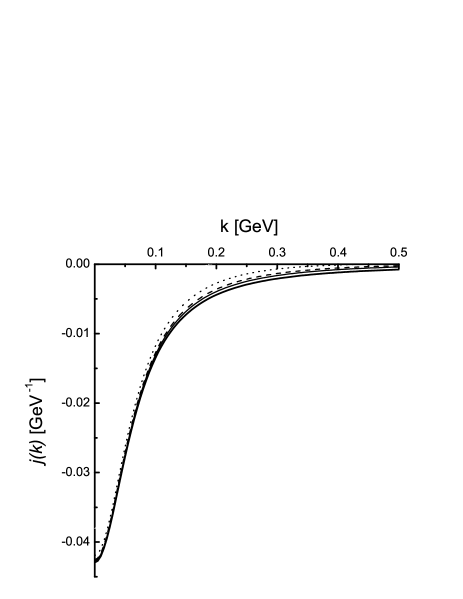
Figure 2: The behaviour of the integrand $j(k)$ of Im$(\hat{J}_{ik})$, as a function of the kaon momentum floating in the loop. We chose $m_{S}=0.98$ GeV, $m_{V}=1.02$ GeV, $m=0.495$ GeV, and four values of the parameter $\beta$: $\beta=0.4$ GeV (dotted line), $\beta=0.6$ GeV (dashed line), $\beta=0.8$ GeV (thin solid line), and $\beta=\infty$ (thick solid line).

We therefore conclude that all results of Ref. mol are valid. In particular, there is no strong suppression of kaon loops by the scalar wave function. Regardless of this, it should be stressed that the data for $\phi\to\gamma a_{0}/f_{0}$ data is very sensitive to the nature of the light scalar mesons, for it allows direct access to the effective coupling constant $g_{\rm eff}$ of the scalar to the kaons. As was shown in Ref. evidence this coupling is a direct measure of the molecular contribution of the scalar mesons.

As a reply to this comment, the authors of the commented paper AK state that, with a properly regularised amplitude $T_{\nu\mu}$ (up to the overall normalisation $T_{\nu\mu}$ coinsides with our $J_{\nu\mu}$ introduced in Eq. (1) above), “the regulator field contribution is caused fully by high momenta ($M\to\infty$) and teaches us how to allow for high $K$ virtualities in gauge invariant way” AK2 . To exemplify their statement, the authors of Ref. AK2 employ the Pauli-Villars regularisation in the full relativistic expression for the amplitude,

$$\overline{T}\left\{\phi(p)\to\gamma[a_{0}(q)/f_{0}(q)],M\right\}=\epsilon^{\nu}(\phi)\epsilon^{\mu}(\gamma)\overline{T}_{\nu\mu}(p,q),$$ (6)

where the overline marks the regularised quantities. In particular, for a quantity

$${\cal O}=\int d^{4}rf(r,p;m),$$ (7)

the corresponding regularised integral reads:

$$\overline{\cal O}(M)=\int d^{4}r[f(r,p;m)-f(r,p;M)],$$ (8)

with $M$ being the regulator mass; the physical amplitude corresponds to the limit $M\to\infty$. Then, by an explicit calculation, the authors of Ref. AK2 find that

$$\epsilon^{\nu}(\phi)\epsilon^{\mu}(\gamma)\overline{T}_{\nu\mu}(p,p)$$ (9)

$$=\epsilon^{\nu}(\phi)\epsilon^{\mu}(\gamma)\left(T^{m}_{\nu\mu}(p,p)-T^{M}_{\nu\mu}(p,p)\right)$$

$$=(\epsilon(\phi)\epsilon(\gamma))(1-1)=0,$$

and thus they conclude that the regularised amplitude is gauge invariant, and this is due to the final subraction coming from the regulator piece. To have a deeper insight, consider $T_{\nu\mu}^{m}(p,p)$ and extract the coefficient of the structure $g_{\mu\nu}$. Then, after using the Feynman parametisation, one has:

$$T^{m}_{\nu\mu}(p,p)=C\left[g_{\mu\nu}\int^{1}_{0}dz\int\frac{d^{4}r}{(2\pi)^{4}}\frac{1}{(r^{2}-R^{2})^{2}}\right.$$

$$-8\int^{1}_{0}dz(1-z)\int\left.\frac{d^{4}r}{(2\pi)^{4}}\frac{r_{\mu}r_{\nu}}{(r^{2}-R^{2})^{3}}\right],$$ (10)

where $C$ is an unimportant numerical coefficient and $R^{2}=z(1-z)p^{2}-m^{2}$. The integrand can be rewritten in the form:

$$\frac{r^{2}g_{\mu\nu}-4r_{\mu}r_{\nu}}{(r^{2}-R^{2})^{3}}-\frac{g_{\mu\nu}R^{2}}{(r^{2}-R^{2})^{3}}.$$ (11)

It is tempting now to perform averaging over the angular variables first, substituting $r_{\mu}r_{\nu}\to\frac{1}{4}r^{2}g_{\mu\nu}$. Then, naively, the first term in the integrand (11) vanishes, whereas the remaining, second term gives a finite constant independent of the mass $m$. Conclusions made by the authors of Ref. AK2 are based on this result, and, finally, they notice that “the finiteness of the subtraction constant hides its high momentum origin”. However, the analysis performed above has a flaw. Indeed, although the angular integration of the first term in (11) gives zero, the remaining radial integral diverges. Therefore, one deals with an undefined expression of the kind $0\times\infty$. In order to resolve this issue, it is important to deal with finite integrals. To this end, we evaluate the integral in $d=4-\epsilon$ dimensions. The radial integral is finite now, whereas the angular integral gives the substitution $r_{\mu}r_{\nu}\to\frac{1}{4-\epsilon}r^{2}g_{\mu\nu}$. It is easy to check that, after taking the limit $\epsilon\to 0$, the contribution of the first term does not vanish any more but, on the contrary, it cancels the contribution of the second term in (11). Thus

$$T^{m}_{\nu\mu}(p,p)=0\quad\mbox{and}\quad T^{M}_{\nu\mu}(p,p)=0$$ (12)

individually. Thus, the apparent contribution of high kaon virtualities found in Ref. AK2 appears as a result of misusing of the Pauli–Villars regularisation scheme, when a regularised finite integral is artificially split into divergent parts and each part is considered separately. In other words, the physical amplitude is given by a sum of several divergent integrals and, in any correct regularisation scheme, these infinite parts cancel each other exactly.

Finally, had the infinitely high momenta been relevant, as advocated in Refs. AK ; AK2 , then the pointlike limit would have rendered useless, as there is no infinitely compact states in nature. This becomes clear when a scalar form factor is introduced, in which case neither dimensional nor Pauli–Villars regularisation is needed. In order to maintain gauge invariance one is forced either to include the diagram (d) of Fig. 1, or to subtract explicitly the amplitude, given by the sum of the diagrams (a)-(c), at $q\to 0$, with both procedures being equivalent. Notice that gauge invariance requires the subtraction of the original amplitude, and not the one with mass $m$ replaced by the (infinitely large) regulator mass $M$. The latter observation invalidates the claim made in Ref. AK2 .

- (1) Yu. S. Kalashnikova, A. E. Kudryavtsev, A. V. Nefediev, J. Haidenbauer, and C. Hanhart, Eur. Phys. J. A 24, 437 (2005).
- (2) E. Marko, S. Hirenzaki, E. Oset, and H. Toki, Phys. Lett. B 470 (1999) 20; J. E. Palomar, S. Hirenzaki, and E. Oset, Nucl. Phys. A 707 (2002) 161; J. E. Palomar, L. Roca, E. Oset, and M. J. Vicente Vacas, Nucl. Phys. A 729 (2003) 743.
- (3) V. E. Markushin, Eur. Phys. J. A 8 (2000) 389.
- (4) J. A. Oller, Phys. Lett. B 426 (1998) 7; Nucl. Phys. A 714 (2003) 161.
- (5) N. N. Achasov and A. V. Kiselev, Phys. Rev. D 76 (2007) 077501
- (6) N. N. Achasov and V. N. Ivanchenko, Nucl. Phys. B 315 (1989) 465.
- (7) S. Nussinov and T.N. Truong, Phys. Rev. Lett. 63 (1989) 1349; (E) Phys. Rev. Lett. 63 (1989) 2002.
- (8) J.L. Lucio and J. Pestieau, Phys. Rev. D 42 (1990) 3253; (E) Phys. Rev. D 43 (1991) 2447.
- (9) A. Bramon, A. Grau, and G. Pancheri, Phys. Lett. B 289 (1992) 97.
- (10) F. E. Close, N. Isgur, and S. Kumano, Nucl. Phys. B 389 (1993) 513.
- (11) F. Gross and D. O. Riska, Phys. Rev. C 36 (1987) 1928; A.N. Kvinikhidze, B. Blankleider, Phys. Rev. C 60 (1999) 044003; Phys. Rev. C 60 (1999) 044004; B. Borasoy, P.C. Bruns, U.-G. Meißner, and R. Nißler, Phys. Rev. C 72 (2005) 065201; C. Hanhart, Yu. S. Kalashnikova, A. E. Kudryavtsev, and A. V. Nefediev, Phys. Rev. D 75 (2007) 074015.
- (12) Yu. S. Kalashnikova, A. E. Kudryavtsev, A. V. Nefediev, J. Haidenbauer, and C. Hanhart, arXiv:hep-ph/0608191.
- (13) F. Ambrosino et al. [KLOE Collaboration], Eur. Phys. J. C 49 (2007) 473.
- (14) V. Baru, J. Haidenbauer, C. Hanhart, Yu. Kalashnikova, and A. E. Kudryavtsev, Phys. Lett. B 586 (2004) 53; C. Hanhart, Eur. Phys. J. A 31 (2007) 543.
- (15) N. N. Achasov and A. V. Kiselev, Phys. Rev. D 78 (2008) 058502.