Algorithm to estimate the Hurst exponent
of high-dimensional fractals

Abstract

We propose an algorithm to estimate the Hurst exponent of high-dimensional fractals, based on a generalized high-dimensional variance around a moving average low-pass filter. As working examples, we consider rough surfaces generated by the Random Midpoint Displacement and by the Cholesky-Levinson Factorization algorithms. The surrogate surfaces have Hurst exponents ranging from $0.1$ to $0.9$ with step $0.1$, and different sizes. The computational efficiency and the accuracy of the algorithm are also discussed.

I Introduction

The scaling properties of random curves and surfaces can be quantified in terms of the Hurst exponent $H$, a parameter defined in the framework of the fractional Brownian walks introduced in Mandelbrot . A fractional Brownian function $f(\bm{r}):\mathbb{R}^{d}\rightarrow\mathbb{R}$, is characterized by a variance $\sigma_{H}^{2}$:

$$\sigma_{H}^{2}=\,\,\left<[f({\bm{r}}+\bm{\lambda})-f(\bm{r})]^{2}\right>\,\,\propto\|\bm{\lambda}\|^{\alpha}\hskip 15.0pt{\rm with}\hskip 10.0pt\alpha=2H\hskip 3.0pt,$$ (1)

with $\bm{r}=(x_{1},x_{2},...,x_{d})$ , $\bm{\lambda}=(\lambda_{1},\lambda_{2},...,\lambda_{d})$ and $\|\bm{\lambda}\|=\sqrt{\lambda_{1}^{2}+\lambda_{2}^{2}+...+\lambda_{d}^{2}}\,$ ; a power spectrum $S_{H}$:

$$S_{H}\propto\|\bm{\omega}\|^{-\beta}\hskip 25.0pt{\rm with}\hskip 15.0pt\beta=d+2H\hskip 3.0pt,$$ (2)

with $\bm{\omega}=(\omega_{1},\omega_{2},...,\omega_{d})$ the angular frequency, $\|\bm{\omega}\|=\sqrt{\omega_{1}^{2}+\omega_{2}^{2}+...+\omega_{d}^{2}}\,$; a number of objects $N_{H}$ of characteristic size $\epsilon$ needed to cover the fractal:

$$N_{H}\propto\epsilon^{-D}\hskip 25.0pt{\rm with}\hskip 15.0ptD=d+1-H\hskip 3.0pt,$$ (3)

$D$ being the fractal dimension of $f({\bm{r}})$. The Hurst exponent ranges from $0$ to $1$, taking the values $H=0.5$, $H>0.5$ and $H<0.5$ respectively for uncorrelated, correlated and anticorrelated Brownian functions.

The application of fractal concepts, through the estimate of $H$, has been proven useful in a variety of fields. For example in $d=1$, heartbeat intervals of healthy and sick hearts are discriminated on the basis of the value of $H$ Thurner ; Goldberger ; the stage of financial market development is related to the correlation degree of return and volatility series Dimatteo ; coding and non coding regions of genomic sequences have different correlation degrees Peng ; climate models are validated by analyzing long-term correlation in atmospheric and oceanographic series Ashkenazy ; Huybers . In $d\geq 2$ fractal measures are used to model and quantify stress induced morphological transformation Blair ; isotropic and anisotropic fracture surfaces Ponson ; Hansen ; Bouchbinder ; Schmittbuhl ; Santucci ; static friction between materials dominated by hard core interactions Sokoloff ; diffusion Levitz ; Malek and transport Oskoee ; Filoche in porous and composite materials; mass fractal features in wet/dried gels Vollet and in physiological organs (e.g. lung) Suki ; hydrophobicity of surfaces with hierarchic structure undergoing natural selection mechanism Yang and solubility of nanoparticles Mihranyan ; digital elevation models Fisher and slope fits of planetary surfaces Sultan-Salem .

A number of fractal quantification methods - based on the Eqs. (1-3) or on variants of these relationships - like Rescaled Range Analysis (R/S), Detrended Fluctuation Analysis (DFA), Detrending Moving Average Analysis (DMA), Spectral Analysis, have been thus proposed to accomplish accurate and fast estimates of $H$ in order to investigate correlations at different scales in $d=1$. A comparatively small number of methods able to capture spatial correlations-operating in $d\geq 2$-have been proposed so far Rangarajan ; Davies ; Alvarez ; Gu ; Kestener ; Alessio ; Carbone ; Arianos . This work is addressed to develop an algorithm to estimate the Hurst exponent of high-dimensional fractals and thus is intended to capture scaling and correlation properties over space. The proposed method is based on a generalized high-dimensional variance of the fractional Brownian function around a moving average. In Section II, we report the relationships holding for fractals with arbitrary dimension. It is argued that the implementation can be carried out in directed or isotropic mode. We show that the Detrending Moving Average (DMA) method Alessio ; Carbone ; Arianos is recovered for $d=1$. In Section III, the feasibility of the technique is proven by implementing the algorithm on rough surfaces - with different size $N_{1}\times N_{2}$ and Hurst exponent $H$ - generated by the Random Midpoint Displacement (RMD) and by the Cholesky-Levinson Factorization (CLF) methods Voss ; Zhou . The generalized variance is estimated over sub-arrays $n_{1}\times n_{2}$ with different size (“scales”) and then averaged over the whole fractal domain $N_{1}\times N_{2}$. This feature reduces the bias effects due to nonstationarity with an overall increase of accuracy - compared to the two-point correlation function, whose average is calculated over all the fractal. Furthermore - compared to the two-point correlation function, whose implementation is carried out along $1$-dimensional lines (e.g. for the fracture problem, the two-point correlation functions are measured along the crack propagation direction and the perpendicular one), the present technique is carried out over $d$-dimensional structures (e.g. squares in $d=2$). In Section IV, we discuss accuracy and range of applicability of the method.

II Method

In order to implement the algorithm, the generalized variance $\sigma^{2}_{DMA}$ is introduced:

$$\sigma^{2}_{DMA}=\frac{1}{\mathcal{N}}\sum_{i_{1}=n_{1}-m_{1}}^{N_{1}-m_{1}}\sum_{i_{2}=n_{2}-m_{2}}^{N_{2}-m_{2}}...\sum_{i_{d}=n_{d}-m_{d}}^{N_{d}-m_{d}}\Big{[}f(i_{1},i_{2},...,i_{d})-\widetilde{f}_{n_{1},n_{2},...n_{d}}(i_{1},i_{2},...,i_{d})\Big{]}^{2}\hskip 3.0pt,$$ (4)

where $f(i_{1},i_{2},...,i_{d})=f(\bm{i})$ is a fractional Brownian function defined over a discrete $d$-dimensional domain, with maximum sizes $N_{1},N_{2},...,\,N_{d}$. It is $i_{1}=1,2,...,\,N_{1}$, $i_{2}=1,2,...,\,N_{2}$, $...$, $i_{d}=1,2,...,\,N_{d}$.   $\bm{n}=(n_{1},n_{2},...,\,n_{d})$ defines the sub-arrays ${\nu}_{d}$ of the fractal domain with maximum values $n_{1max}=\mathrm{max}\{n_{1}\}$,  $n_{2max}=\mathrm{max}\{n_{2}\},...$,  $n_{dmax}=\mathrm{max}\{n_{d}\}$; $m_{1}=\mathrm{int}(n_{1}\theta_{1})$, $m_{2}=\mathrm{int}(n_{2}\theta_{2})$,…, $m_{d}=\mathrm{int}(n_{d}\theta_{d})$ and $\theta_{1}$, $\theta_{2}$,  $...\,\theta_{d}$ are parameters ranging from 0 to 1; ${\mathcal{N}}={(N_{1}-n_{1max})\cdot(N_{2}-n_{2max})\cdot...\cdot(N_{d}-n_{dmax})}$. The function $\widetilde{f}_{n_{1},n_{2},...,\,n_{d}}(i_{1},i_{2},...,i_{d})=\widetilde{f}$ is given by:

$$\widetilde{f}_{n_{1},n_{2},...,\,n_{d}}(i_{1},i_{2},...,\,i_{d})=\frac{1}{n_{1}n_{2}...n_{d}}\sum_{k_{1}=-m_{1}}^{n_{1}-1-m_{1}}\sum_{k_{2}=-m_{2}}^{n_{2}-1-m_{2}}...$$

$$...\sum_{k_{d}=-m_{d}}^{n_{d}-1-m_{d}}f(i_{1}-k_{1},i_{2}-k_{2},...,i_{d}-k_{d})\hskip 3.0pt,$$ (5)

that is an average of $f$ calculated over the sub-arrays ${\nu}_{d}$. The Eqs. (4) and (II) are defined for any value of $n_{1},n_{2},...,\,n_{d}$ and for any shape of the sub-arrays, however, it is preferable to choose sub-arrays with $n_{1}=n_{2}=....=n_{d}$ to avoid spurious directionality in the results. The generalized variance $\sigma^{2}_{DMA}$ varies as $(\sqrt{n_{1}^{2}+n_{2}^{2}+...+n_{d}^{2}}\,)^{2H}$ as a consequence of the property (1) of the fractional Brownian functions.

Upon variation of the parameters $\theta_{1}$, $\theta_{2}\,,...\,,\theta_{d}$ in the range $\left[0,1\right]$, the indexes $i_{1},i_{2},...,\,i_{d}$ and $k_{1}$, $k_{2}\,,...\,,k_{d}$ of the sums in the Eqs. (4) and (II) are accordingly set within ${\nu}_{d}$. In particular, $(i_{1},i_{2},...,\,i_{d})$ coincides respectively with: (a) one of the vertices of ${\nu}_{d}$ for $\theta_{1}=\theta_{2}=...=\theta_{d}=0$ and $\theta_{1}=\theta_{2}=...=\theta_{d}=1$ or (b) the center of ${\nu}_{d}$ for $\theta_{1}=\theta_{2}=...=\theta_{d}=1/2$. It is worthy of note that the choice $\theta_{1}=\theta_{2}=...=\theta_{d}=1/2$ corresponds to the isotropic implementation of the algorithm, while $\theta_{1}=\theta_{2}=...=\theta_{d}=0$ and $\theta_{1}=\theta_{2}=...=\theta_{d}=1$ correspond to the directed implementation. For example in $d=2$, the isotropic implementation implies that the variance defined by the Eq. (4) is referred to a moving average $\widetilde{f}$ calculated over squares $n_{1}\times n_{2}$ whose center is $(i_{1},i_{2})$. Conversely, the directed implementation implies that the function $\widetilde{f}$ is calculated over squares $n_{1}\times n_{2}$ with one of the vertices in $(i_{1},i_{2})$. The directed mode is of interest to estimate $H$ in fractals with preferential growth direction, e.g. biological tissues (lung), epitaxial layers, crack propagation in fracture (anisotropic fractals). If the fractal is isotropic and the accuracy is a priority, the parameters $\theta_{1},\theta_{2},...,\theta_{d}$ should be preferably taken equal to $1/2$ to achieve the most precise estimate of $H$. The dependence of the algorithm on $\theta$ for $d=1$ has been discussed in Arianos .

In order to calculate the Hurst exponent, the algorithm is implemented through the following steps. The moving average $\widetilde{f}$ is calculated for different sub-arrays ${\nu}_{d}$, by varying $n_{1},n_{2},...,\,n_{d}$ from 2 to the maximum values $n_{1max},n_{2max},...,\,n_{dmax}$. The values $n_{1max},n_{2max},...,\,n_{dmax}$ depend on the maximum size of the fractal domain. In order to minimize the saturation effects due to finite-size, it should be: $n_{1max}<<N_{1}$; $n_{2max}<<N_{2};...;\,n_{dmax}<<N_{d}$. These constraints will be further clarified in Section III, where the algorithm is implemented over fractal surfaces with different sizes. For each sub-array ${\nu}_{d}$, the corresponding value of $\sigma_{DMA}^{2}$ is calculated and finally plotted on log-log axes.

To elucidate the way the algorithm works, in the following we consider its implementation for $d=1$ and $d=2$. The case $d=1$ reduces to the Detrending Moving Average (DMA) method already used for long-range correlated time series Alessio ; Carbone ; Arianos .

1-dimensional case:

By posing $d=1$ in the Eq. (4), one obtains:

$$\sigma^{2}_{DMA}=\frac{1}{N_{1}-n_{1max}}\sum_{i_{1}=n_{1}-m_{1}}^{N_{1}-m_{1}}\Big{[}f(i_{1})-\tilde{f}_{n_{1}}(i_{1})\Big{]}^{2}\hskip 3.0pt,$$ (6)

where $N_{1}$ is the length of the sequence, $n_{1}$ is the sliding window and $n_{1max}=\mathrm{max}\{n_{1}\}\ll N_{1}$. The quantity $m_{1}=\mathrm{int}(n_{1}\theta_{1})$ is the integer part of $n_{1}\theta_{1}$ and $\theta_{1}$ is a parameter ranging from 0 to 1. The relationship (6) defines a generalized variance of the sequence $f(i_{1})$ with respect to the function $\widetilde{f}_{n_{1}}(i_{1})$:

$$\widetilde{f}_{n_{1}}(i_{1})=\frac{1}{n_{1}}\sum_{k_{1}=-m_{1}}^{n_{1}-1-m_{1}}f(i_{1}-k_{1})\hskip 3.0pt,$$ (7)

which is the moving average of $f(i_{1})$ over each sliding window of length $n_{1}$. The moving average $\widetilde{f}_{n_{1}}(i_{1})$ is calculated for different values of the window $n_{1}$, ranging from 2 to the maximum value $n_{1max}$. The variance $\sigma_{DMA}^{2}$ is then calculated according to the Eq. (6) and plotted as a function of $n_{1}$ on log-log axes. The plot is a straight line, as expected for a power-law dependence of $\sigma_{DMA}^{2}$ on $n_{1}$:

$$\sigma_{DMA}^{2}\sim n_{1}^{2H}\hskip 3.0pt.$$ (8)

The Eq. (8) allows one to estimate the scaling exponent $H$ of the series $f(i_{1})$. Upon variation of the parameter $\theta_{1}$ in the range $\left[0,1\right]$, the index $k_{1}$ in $\widetilde{f}_{n_{1}}(i_{1})$ is accordingly set within the window $n_{1}$. In particular, $\theta_{1}=0$ corresponds to average ${f}_{n_{1}}(i_{1})$ over all the points to the left of $i_{1}$ within the window $n_{1}$; $\theta_{1}=1$ corresponds to average ${f}_{n_{1}}(i_{1})$ over all the points to the right of $i_{1}$ within the window $n_{1}$; $\theta_{1}=\frac{1}{2}$ corresponds to average ${f}_{n_{1}}(i_{1})$ with the reference point in the center of the window $n_{1}$.

2-dimensional case

For $d=2$, the generalized variance defined by the Eq.(4) writes:

$$\sigma^{2}_{DMA}=\frac{1}{(N_{1}-n_{1max})(N_{2}-n_{2max})}\sum_{i_{1}=n_{1}-m_{1}}^{N_{1}-m_{1}}\sum_{i_{2}=n_{2}-m_{2}}^{N_{2}-m_{2}}\Big{[}f(i_{1},i_{2})-\widetilde{f}_{n_{1},n_{2}}(i_{1},i_{2})\Big{]}^{2}\hskip 3.0pt,$$ (9)

with $\widetilde{f}_{n_{1},n_{2}}(i_{1},i_{2})$ given by:

$$\widetilde{f}_{n_{1},n_{2}}(i_{1},i_{2})=\frac{1}{n_{1}n_{2}}\sum_{k_{1}=-m_{1}}^{n_{1}-1-m_{1}}\sum_{k_{2}=-m_{2}}^{n_{2}-1-m_{2}}f(i_{1}-k_{1},i_{2}-k_{2})\hskip 5.0pt.$$ (10)

The average $\widetilde{f}$ is calculated over sub-arrays with different size $n_{1}\times n_{2}$. The next step is the calculation of the difference $f(i_{1},i_{2})-\widetilde{f}_{n_{1},n_{2}}(i_{1},i_{2})$ for each sub-array $n_{1}\times n_{2}$. A log-log plot of $\sigma_{DMA}^{2}$:

$$\sigma_{DMA}^{2}\sim\left[\sqrt{n_{1}^{2}+n_{2}^{2}}\right]^{2H}\sim{s}^{H}\hskip 5.0pt.$$ (11)

as a function of $s=n_{1}^{2}+n_{2}^{2}$, yields a straight line with slope $H$.

Depending upon the values of the parameters $\theta_{1}$ and $\theta_{2}$, entering the quantities $m_{1}=\mathrm{int}(n_{1}\theta_{1})$ and $m_{2}=\mathrm{int}(n_{2}\theta_{2})$ in the Eqs. (9,10), the position of $(k_{1},k_{2})$ and $(i_{1},i_{2})$ can be varied within each sub-array. $(i_{1},i_{2})$ coincides with a vertex of the sub-array if: (i) $\theta_{1}=0$, $\theta_{2}=0$; (ii) $\theta_{1}=0$, $\theta_{2}=1$; (iii) $\theta_{1}=1$, $\theta_{2}=0$; (iv) $\theta_{1}=1$, $\theta_{2}=1$ (directed implementation). The choice $\theta_{1}=\theta_{2}=1/2$ corresponds to take the point $(i_{1},i_{2})$ coinciding with the center of each sub-array $n_{1}\times n_{2}$ (isotropic implementation) note1 .

III Results

In order to test feasibility and robustness of the proposed method, synthetic rough surfaces with assigned Hurst exponents have been generated by the Random Midpoint Displacement (RMD) algorithm and by the Cholesky-Levinson Factorization (CLF) method Voss ; Zhou . The widespread use of the RMD algorithm is based on the trade-off of its fast, simple and efficient implementation to its limited accuracy especially for $H\ll 0.5$ and $H\gg 0.5$. Conversely, the Cholesky-Levinson Factorization method is one of the most accurate techniques to generate $1d$ and $2d$ fractional Brownian functions, at the expenses of a more complex implementation structure note2 .

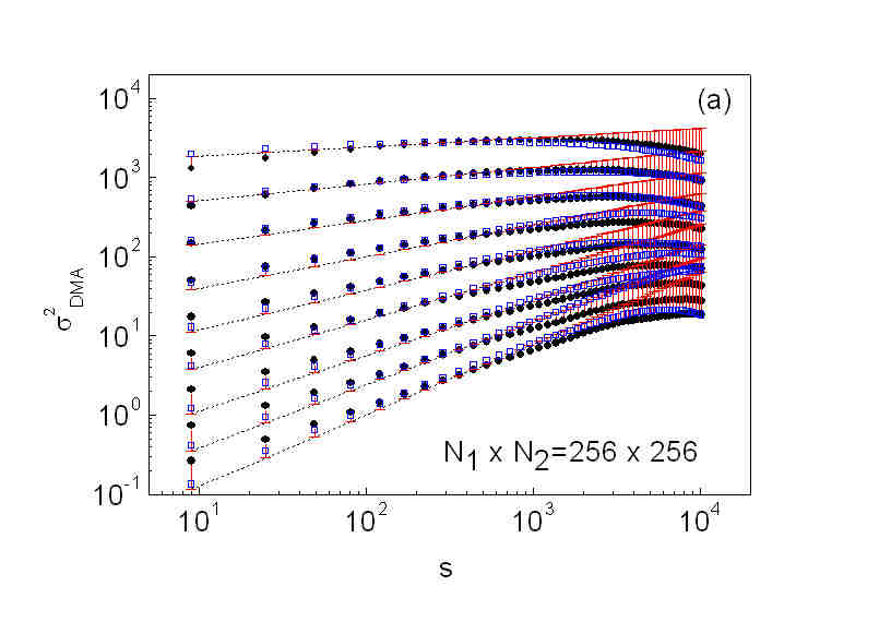
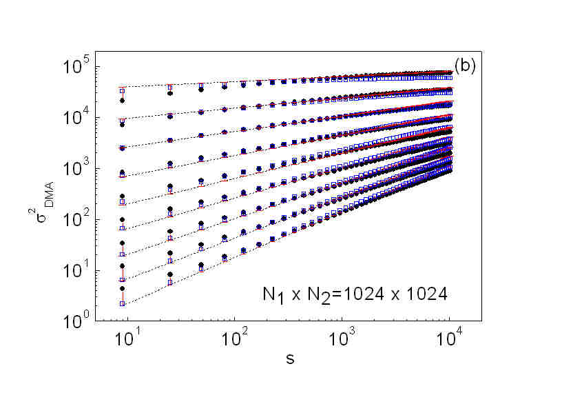
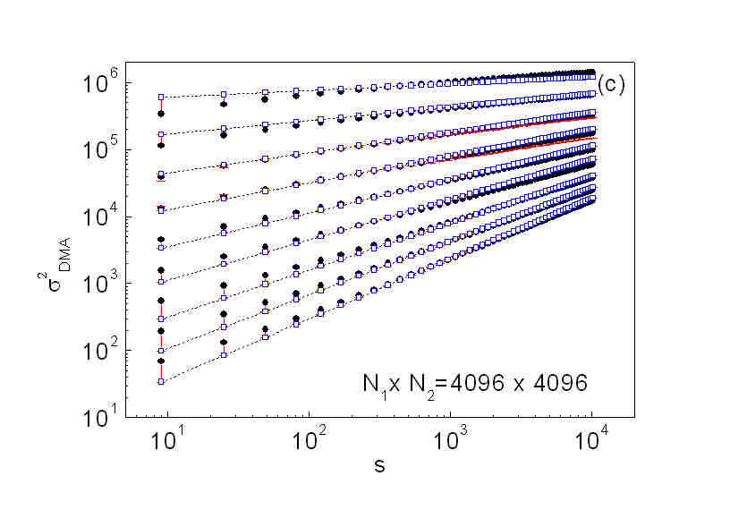
Figure 1: (Color online) Log-log plot of $\sigma^{2}_{DMA}$ for fractal surfaces respectively with size $N_{1}\times N_{2}=256\times 256$ (a), $N_{1}\times N_{2}=1024\times 1024$ (b) and $N_{1}\times N_{2}=4096\times 4096$ (c). The data refer to fractal surfaces generated by the RMD (circles) and by the CLF (squares) methods. The Hurst exponent $H_{in}$ - input of the RMD and the CLF algorithm - varies from $0.1$ to $0.9$ with step $0.1$. The results correspond to the isotropic implementation, i.e. with the parameters $\theta_{1}=\theta_{2}=1/2$ in the Eq.(9). The dashed lines represent the behavior expected for full linearity, i.e. the log-log plot of curves varying as $s^{H_{in}}$. It is worthy of note that the CLF data are closer to the full-linearity compared to the RMD ones.

In Fig. 1, the log-log plots of $\sigma^{2}_{DMA}$ as a function of $s$ are shown for the synthetic fractal surfaces generated by the RMD (circles) and by the CLF method (squares). The surfaces have Hurst exponents $H_{in}$ ranging from $0.1$ to $0.9$ with step $0.1$. The domain sizes are respectively $N_{1}\times N_{2}=256\times 256$ (a), $N_{1}\times N_{2}=1024\times 1024$ (b) and $N_{1}\times N_{2}=4096\times 4096$ (c). The dashed lines show the behavior that should be exhibited by variances varying exactly as $s^{H_{in}}$ over the entire range of scales. The plots of $\sigma^{2}_{DMA}$ as a function $s$ are in good agreement with the behavior expected on the basis of the Eq. (11). The quality of the fits is higher for the surfaces generated by the CLF method, confirming that the RMD algorithm synthesizes less accurate fractals. By comparing the results of the simulation (symbols) to the straight lines corresponding to full linearity over the whole range (dashed), deviations from the full linearity can be observed especially for the small surfaces at the extremes of the scale. A plot of the slopes for the fractal surfaces generated by the CLF algorithm is shown in Fig. 2 for different sizes of the fractal domain. A detailed discussion of the origin of the deviations at low and large scales is reported in the Section IV.

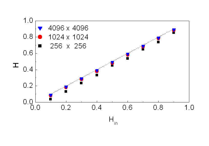
Figure 2: (Color online) Plot of the values of $H$ obtained by linear fit of the curves shown in Fig. 1 (a), (b), (c). The data refer to the fractal surfaces generated by the Cholesky-Levinson Factorization method (squares). The dashed lines represent the ideal behavior: $H=H_{in}$.

Finally, we also show three examples of digital images currently mapped to fractal surfaces with reference to the color intensity i.e. to the levels of Red, Green and Blue (RGB). The Hurst exponents estimated by the proposed method are respectively $H=0.1$ (a), $H=0.5$ (b) and $H=0.9$ (c) for the images in Fig. 3.

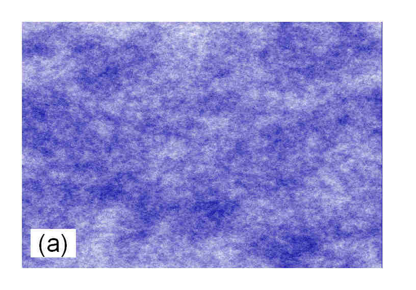
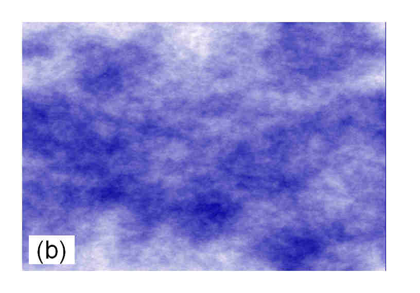
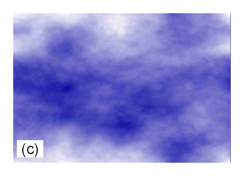
Figure 3: (Color online). Cloudy sky images respectively with Hurst exponent $H=0.1$ (a), $H=0.5$ (b) and $H=0.9$ (c). Such heterogeneous images are represented as fractal surfaces by mapping the color intensity (RGB content).

IV Discussion

The proposed algorithm is characterized by short execution time and ease of implementation. By considering the case $d=2$, the function $\widetilde{f}_{n_{1},n_{2}}(i_{1},i_{2})$ is indeed simply obtained by summing the values of $f(i_{1},i_{2})$ over each sub-array $n_{1}\times n_{2}$. Then the sum is updated at each step by adding the last and discarding the first row (column) of each sliding array $n_{1}\times n_{2}$. For higher dimensions, the sum is updated at each step by adding and discarding a $d-1$ dimensional set of each array $n_{1}\times n_{2}\times...\times n_{d}$. The algorithm does not use arbitrary parameters, the computation simply relying on averages of $f$. We will now argue on the origin of the deviations at small and at large scales.

Deviations at large scales. The deviations from the linearity at large scales, leading to the saturation of the $\sigma^{2}_{DMA}$, are due to finite size effects. The small surfaces do not contain enough data to make the evaluation of the scaling law over the sub-arrays statistically meaningful. By comparing the data in Figs. 1 (a), (b), (c), one can note that the saturation effect decreases upon increasing the size $N_{1}\times N_{2}$ of the fractal surface. The finite size effects become negligible when the conditions $n_{1max}<<N_{1}$; $n_{2max}<<N_{2};...;\,n_{dmax}<<N_{d}$ are fulfilled.

Deviations occurring at small scales. The deviations occurring at low scales are related to the departure of the low-pass filter from the ideality. This problem also occurs with one-dimensional fractals (time series) resulting in the quite generally reported overestimation of $H$ in anticorrelated signals and underestimation of $H$ in correlated signals Caccia ; Hu ; Chen ; Xu ; Stoev . We will discuss the origin of these deviations by means of the filter transfer function $\mathcal{H}_{\mathcal{T}}(\omega)$ Hamming . The algorithm is based on a generalized variance of the function $f$ with respect to $\widetilde{f}$. The function $\widetilde{f}$ is the output of a low-pass filter driven by $f$, with impulse response a box-car function. In the Appendix, the transfer function $\mathcal{H}_{\mathcal{T}}(\omega)$ of $\widetilde{f}$ is explicitly calculated and shown in Fig.(4) for $d=2$. For an ideal low-pass filter, the transfer function should be one or zero respectively at frequencies lower or higher than the cut-off frequency. However, in real low-pass filters, at frequencies lower than the cut-off frequency, all the components of the signal suffer some attenuation but $\omega=0$. The cut-off frequencies of $\mathcal{H}_{\mathcal{T}}(\omega)$ are $\omega_{i}=\pi/\tau_{i}$, i.e. the first zeroes of the functions ${\sin\omega_{i}\tau_{i}}/{\omega_{i}\tau_{i}}$ in the Eq. (16). Moreover, in real filters, at frequencies higher than $\pi/\tau_{i}$, due to the presence of the sidelobes, components of the signals lying in the bands $(\pi/\tau_{i},2\pi/\tau_{i});(2\pi/\tau_{i},3\pi/\tau_{i});...$, are not fully filtered out. As a result, the function $\widetilde{f}$ contains: (a) less components with frequency lower than $\omega_{i}=\pi/\tau_{i}$ and (b) more components with frequency higher than $\omega_{i}=\pi/\tau_{i}$ compared to what it would be expected with an ideal low-pass filter. The lack of low-frequency components depends on the central lobe, while the excess of high-frequency components depends on the side lobes. The excess of high-frequency components results in a smaller value of the difference $f-\widetilde{f}$, i.e. in a decrease of $\sigma_{DMA}^{2}$ and, thus, in an increase of the slope of the log-log plot. Conversely, the lack of low-frequency components results in a larger value of the difference $f-\widetilde{f}$, i.e. in an increase of $\sigma_{DMA}^{2}$ and, thus, in a decrease of the slope of the log-log plot. The two effects are more relevant with smaller values of the scales, when the filter nonideality is greater. Moreover, as one can deduce from the Eqs. (2) and (18), the effect of the side lobes dominates in high-frequency rich fractals with $H<0.5$, while the effect of the central lobe is dominant in fractals with $H>0.5$, rich of low-frequency components.

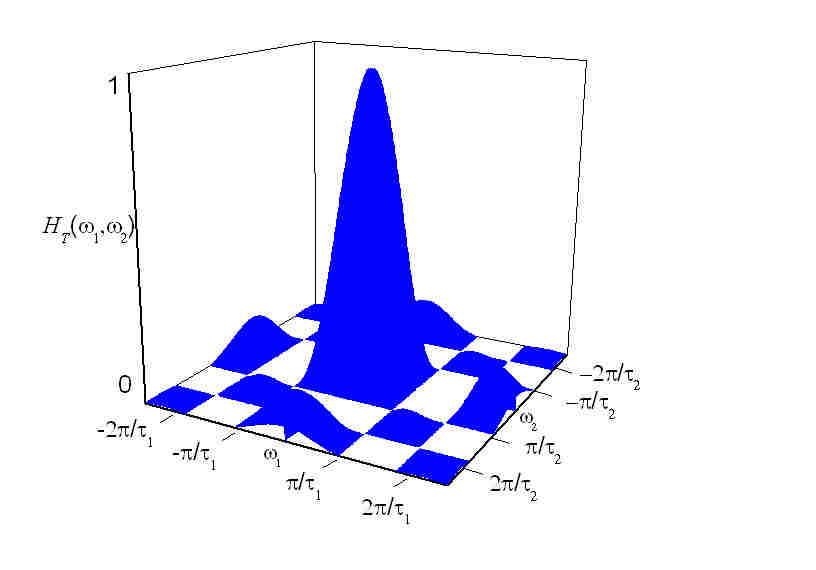
Figure 4: (Color online) Plot of the transfer function $\mathcal{H}_{\mathcal{T}}(\omega_{1},\omega_{2})$.

Table 1: Slopes $H_{I}$, $H_{II}$, $H_{III}$ and relative errors $\Delta H_{I}$, $\Delta H_{II}$, $\Delta H_{III}$ of the curves plotted in Fig. 1(b) (squares). The slopes have been calculated by linear fit respectively over the ranges: $10\leq s\leq 100$ ($H_{I}$), $10\leq s\leq 1000$ ($H_{II}$) and $10\leq s\leq 10000$ ($H_{III}$). The errors $\Delta H_{I}$, $\Delta H_{II}$, $\Delta H_{III}$ are calculated as $\Delta H=(H-H_{in})/H_{in}$.

$H_{in}$	$H_{I}$	$\Delta H_{I}$	$H_{II}$	$\Delta H_{II}$	$H_{III}$	$\Delta H_{III}$
0.1	$0.1346$	$+3.46\cdot 10^{-1}$	$0.1073$	$+7.30\cdot 10^{-2}$	0.0718	$-2.822\cdot 10^{-1}$
0.2	$0.2272$	$+1.36\cdot 10^{-1}$	$0.2050$	$+2.50\cdot 10^{-2}$	0.1700	$-1.500\cdot 10^{-1}$
0.3	$0.3233$	$+7.77\cdot 10^{-2}$	$0.2995$	$-1.67\cdot 10^{-3}$	0.2716	$-9.467\cdot 10^{-2}$
0.4	$0.4205$	$+5.12\cdot 10^{-2}$	$0.3970$	$-7.50\cdot 10^{-3}$	0.3691	$-7.725\cdot 10^{-2}$
0.5	$0.5178$	$+3.56\cdot 10^{-2}$	$0.4973$	$-5.40\cdot 10^{-3}$	0.4752	$-4.960\cdot 10^{-2}$
0.6	$0.6171$	$+2.85\cdot 10^{-2}$	$0.5973$	$-4.50\cdot 10^{-3}$	0.5617	$-6.383\cdot 10^{-2}$
0.7	$0.7185$	$+2.64\cdot 10^{-2}$	$0.6956$	$-6.29\cdot 10^{-3}$	0.6770	$-3.286\cdot 10^{-2}$
0.8	$0.8207$	$+2.58\cdot 10^{-2}$	$0.7999$	$-1.25\cdot 10^{-4}$	0.7659	$-4.263\cdot 10^{-2}$
0.9	$0.9253$	$+2.81\cdot 10^{-2}$	$0.8999$	$-1.11\cdot 10^{-4}$	0.8679	$-3.567\cdot 10^{-2}$

In order to gain further insight in the above theoretical arguments, we report in Table 1 the slopes $H_{I}$, $H_{II}$ and $H_{III}$ of the curves (squares) plotted in Fig. 1 (b)) over different ranges. The slopes have been calculated by linear fit respectively over the ranges $10\leq s\leq 100$ ($H_{I}$), $10\leq s\leq 1000$ ($H_{II}$) and $10\leq s\leq 10000$ ($H_{III}$). The relative errors $\Delta H=(H-H_{in})/H_{in}$ are given respectively in the $3^{rd}$, $5^{th}$ and $7^{th}$ columns. The slope $H_{I}$ is greater than the expected value $H_{in}$. The slope $H_{II}$ is overestimated for $H=0.1$ and $H=0.2$ and underestimated for $H>0.2$. The slope $H_{III}$ is underestimated since the effects of the finite-size of the fractal domain play a dominant role.

We address the question if the artifacts due to the filter nonideality described above might be corrected somehow. In the remaining of this section, we will thus consider the use of windows whose general effect is to increase the width of the central lobe while reducing those of the sidelobes of the function $\mathcal{H}_{\mathcal{T}}(\omega)$ (a detailed description of these methods can be found in Hamming ). By restricting our discussion to the present technique, the correction is performed by using the following variant of the relationship (II):

$$\widetilde{f}^{\star}_{n_{1},n_{2},...,\,n_{d}}(i_{1},i_{2},...,\,i_{d})= (1-\alpha)f_{n_{1},n_{2},...,\,n_{d}}(i_{1},i_{2},...,\,i_{d})$$ (12)

$$+\alpha\widetilde{f}_{n_{1},n_{2},...,\,n_{d}}(i_{1}-1,i_{2}-1,...,\,i_{d}-1)\hskip 3.0pt,$$

where $\alpha=n_{1}n_{2}...n_{d}/[(n_{1}+1)(n_{2}+1)...(n_{d}+1)]$. The Eq. (12) reduces for $d=1$ to the exponentially weighted moving average (EWMA). In practice, the difference between the Eq. (II) and the Eq. (12) is that the function $\widetilde{f}^{\star}$ places more importance to the data around the point $i_{1},i_{2},...,\,i_{d}$. This is achieved by assigning to the function a weight $(1-\alpha)$, while all the other values are summed together and weighted by $\alpha$. In Fig. 5, we show the ratio $\sigma^{2}_{DMA}/s^{H_{in}}$ obtained by implementing the algorithm respectively with the function $\widetilde{f}$ (solid lines) and $\widetilde{f}^{\star}$ (dashed lines) in the range $10\leq s\leq 100$. The ratio $\sigma^{2}_{DMA}/s^{H_{in}}$ is noticeably closer to a constant value when the function $\widetilde{f}$ is replaced by $\widetilde{f}^{\star}$, with a corresponding reduction of two orders of magnitude in the relative error $\Delta H_{I}$.

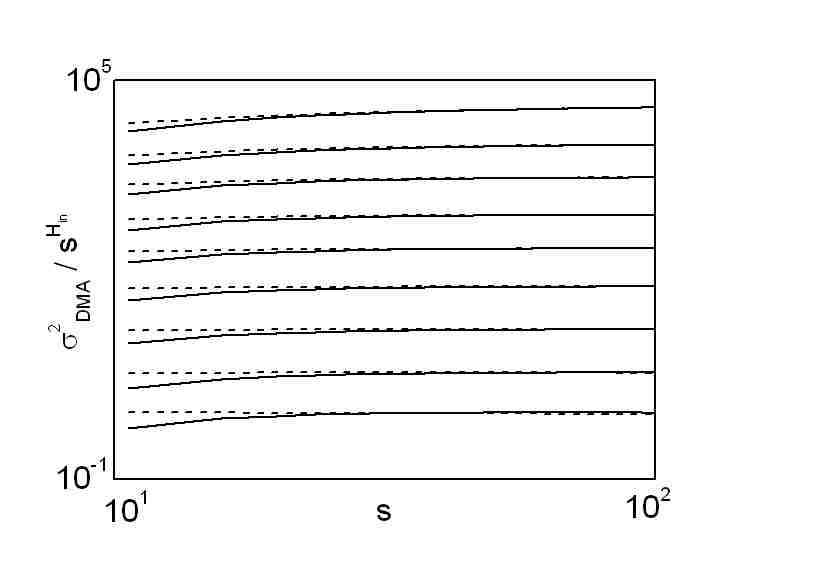
Figure 5: (Color online) Plot of the function $\sigma^{2}_{DMA}$ with $\widetilde{f}$ defined by the Eq. (4) (solid lines) and $\widetilde{f}^{\star}$ defined by the Eq. (12) (dashed lines). It can be noted that the deviations of the slope at small scales are reduced by the use of $\widetilde{f}^{\star}$ implying a corresponding reduction of the relative error $\Delta H_{I}$ of two orders of magnitude.

V Conclusion

We have put forward an algorithm to estimate the Hurst exponent of fractals with arbitrary dimension, based on the high-dimensional generalized variance $\sigma^{2}_{DMA}$ defined by the Eq. (4).

The methods currently used to estimate the Hurst exponent of high-dimensional fractals are based on: (i) $1-d$ two-point correlation and structure functions operated along different directions, (ii) high$-d$ Fourier and wavelet transforms Ponson ; Hansen ; Bouchbinder ; Schmittbuhl ; Santucci ; Kestener . The advantage of the methods (i) is the ease of implementation. Their drawback is the limited accuracy due to biases and nonstationarities, being these functions calculated over the entire fractal domain. The methods (ii) are more accurate, however their implementation is complicated especially for data set with limited extension. The generalized variance $\sigma_{DMA}^{2}$ is “scaled”, meaning that it is calculated over sub-arrays of the whole fractal domain by means of the function $\widetilde{f}$. The “scales” are set by the size of the sub-arrays $n_{1}\times n_{2}\times....\times n_{d}$. Therefore, the proposed method exhibits at the same time: (a) ease of implementation, being based on a variance-like approach and (b) high accuracy, being calculated over scaled sub-arrays rather than on the whole fractal domain.

A further important feature of the proposed algorithm is that it can be implemented “isotropically” or in “directed” mode to accomplish estimates of $H$ in fractals having preferential growth direction e.g. biological tissues, epitaxial layers or in crack propagation in fracture. The isotropic implementation is obtained by taking $\theta_{1}=\theta_{2}=...=\theta_{d}=1/2$ in the Eq. (4). This choice implies that the reference point $(i_{1},i_{2},...,i_{d})$ of the moving average lies in the center of each sub-array $n_{1}\times n_{2}\times...\times n_{d}$ and thus $\widetilde{f}$ is calculated by summing the values of $f$ around $(i_{1},i_{2},...,i_{d})$. Conversely, to implement the algorithm in a preferential direction (directed implementation), the reference point must be coincident with one of extremes of the segment $n_{1}$, or with one of the vertices of the square grid $n_{1}\times n_{2}$ or of the d-dimensional array $n_{1}\times n_{2}\times...\times n_{d}$. The directed implementation can be performed by choosing for example $\theta_{1}=\theta_{2}=...=\theta_{d}=0$.

Further generalizations of the proposed method can be envisaged for applications to the analysis of time-dependent spatial correlations in $d\geq 2$.

*

Appendix A Transfer Function of $\widetilde{f}$

The function $\widetilde{f}$, defined by the Eq. (II), corresponds to the discrete form of the integral:

$$\widetilde{f}(x_{1},x_{2},...,\,x_{d})=\frac{1}{\tau_{1}\tau_{2}...\tau_{d}}\int_{x_{1}-\tau_{1}}^{x_{1}}\!dx_{1}^{\prime}$$

$$\int_{x_{2}-\tau_{2}}^{x_{2}}\!dx_{2}^{\prime}\,...\int_{x_{d}-\tau_{d}}^{x_{d}}dx_{d}^{\prime}f(x_{1}^{\prime},x_{2}^{\prime},...,x_{d}^{\prime})$$ (13)

where for the sake of simplicity we have considered the case $\theta_{1}=\theta_{2}=,...,=\theta_{d}=0$.

The Eq. (A) can be rewritten as a convolution integral:

$$\widetilde{f}(x_{1},x_{2},...,\,x_{d})=\frac{1}{\tau_{1}\tau_{2}...\tau_{d}}\int_{-\infty}^{\infty}dx_{1}^{*}\,U\!\!\left(\frac{x_{1}^{*}}{{\tau_{1}}}\right)\int_{-\infty}^{\infty}dx_{2}^{*}\,U\!\!\left(\frac{x_{2}^{*}}{\tau_{2}}\right)...$$

$$...\int_{-\infty}^{\infty}dx_{d}^{*}\,U\!\!\left(\frac{x_{d}^{*}}{{\tau_{d}}}\right)f(x_{1}-x_{1}^{*},x_{2}-x_{2}^{*},...,\,x_{d}-x_{d}^{*})$$ (14)

with the convolution kernels given by the boxcar function:

$$U(x_{i}^{*}/\tau_{i})=\begin{cases}&1\hskip 5.0pt{\rm for}\hskip 5.0pt0<x^{*}/\tau_{i}<1\\ &0\hskip 5.0pt{\rm elsewhere}\hskip 5.0pt.\\ \end{cases}$$

The transfer function can be calculated as follows:

$$\mathcal{H}_{\mathcal{T}}(\omega_{1},\omega_{2},...\,,\omega_{d})=\frac{1}{\tau_{1}\tau_{2}...\tau_{d}}\int_{0}^{\tau_{1}}dx_{1}\int_{0}^{\tau_{2}}dx_{2}\,...$$

$$\int_{0}^{\tau_{d}}dx_{d}\exp[-i2\pi(\omega_{1}x_{1}+\omega_{2}x_{2}+...+\omega_{d}x_{d})]$$ (15)

that can be written as:

$$\mathcal{H}_{\mathcal{T}}(\omega_{1},\omega_{2},...,\omega_{d})=\prod_{i=1}^{d}\frac{\sin\omega_{i}\tau_{i}}{\omega_{i}\tau_{i}}$$ (16)

that is thus $d$-times the function ${\sin\omega_{i}\tau_{i}}/{\omega_{i}\tau_{i}}$.

The Fourier transform $\widetilde{\mathcal{F}}$ of the function $\widetilde{f}$ can be obtained by means of the following relationship:

$$\widetilde{\mathcal{F}}(\omega_{1},\omega_{2},...,\,\omega_{d})=\mathcal{H}_{\mathcal{T}}(\omega_{1},\omega_{2},...,\,\omega_{d})\mathcal{F}(\omega_{1},\omega_{2},...\omega_{d})$$ (17)

where $\mathcal{F}(\omega_{1},\omega_{2},...,\omega_{d})$ is the Fourier transform of the function $f(x_{1},x_{2},...,\,x_{d})$.

The power spectrum ${\widetilde{S}}$ of the function $\widetilde{f}$ is given by:

$${\widetilde{S}}(\omega_{1},\omega_{2},...,\omega_{d})=|\mathcal{H}_{\mathcal{T}}(\omega_{1},\omega_{2},...,\omega_{d})|^{2}S(\omega_{1},\omega_{2},...,\omega_{d})$$ (18)

where $S(\omega_{1},\omega_{2},...,\omega_{d})$ is the power spectrum of the function $f(x_{1},x_{2},...,x_{d})$.

References

- (1) B. B. Mandelbrot and J. W. Van Ness, SIAM Rev. 4, 422 (1968).
- (2) S. Thurner, M. C. Feurstein, and M. C. Teich, Phys. Rev. Lett. 80, 1544 (1998).
- (3) A. L. Goldberger, L. A. N. Amaral, J. M. Hausdorff, P. Ch. Ivanov, C.-K. Peng, and H. E. Stanley, Proc. Natl. Acad. Sci. 99, 2466 (2002).
- (4) T. Di Matteo, T. Aste, M. M. Dacorogna, J. Banking & Finance 29, 827 (2005).
- (5) C. K. Peng, S. V. Buldyrev, S. Havlin, M. Simons, H. E. Stanley, and A. L. Goldberger, Phys. Rev. E 49, 1685 (1994).
- (6) Y. Ashkenazy, D. Baker, H. Gildor, S. Havlin, Geophys. Res. Lett. 30, 2146 (2003).
- (7) P. Huybers, W. Curry, Nature 441, 7091 (2006).
- (8) D. L. Blair and A. Kudrolli, Phys. Rev. Lett. 94, 166107 (2005).
- (9) L. Ponson, D. Bonamy, and E. Bouchaud, Phys. Rev. Lett. 96, 035506 (2006).
- (10) A. Hansen, G. G. Batrouni, T. Ramstad and J. Schmittbuhl, Phys. Rev. E 75, 030102(R) (2007).
- (11) E. Bouchbinder, I. Procaccia, S. Santucci, and L. Vionel, Phys. Rev. Lett. 96, 055509 (2006).
- (12) J. Schmittbuhl, F. Renard, J. P. Gratier, and R. Toussaint, Phys. Rev. Lett. 93, 238501 (2004).
- (13) S. Santucci, K.J. Maloy, A. Delaplace, et al. , Phys. Rev. E 75, 016104 (2007).
- (14) J.B. Sokoloff, Phys. Rev. E 73, 016104 (2006).
- (15) P. Levitz, D. S. Grebenkov, M. Zinsmeister, K. M. Kolwankar and B. Sapoval, Phys. Rev. Lett., 96, 180601 (2006).
- (16) K. Malek and M.O. Coppens, Phys. Rev. Lett. 87, 125505 (2001).
- (17) E. N. Oskoee and M. Sahimi, Phys. Rev. B 74, 045413 (2006).
- (18) M. Filoche and B. Sapoval, Phys. Rev. Lett. 84, 5776 (2000).
- (19) D. R. Vollet, D. A. Donati, A. Ibanez Ruiz, and F. R. Gatto, Phys. Rev. B 74, 024208 (2006).
- (20) B. Suki, A.-L. Barabasi, Z. Hantos, F. Petak, and H. E. Stanley, Nature 368, 615 (1994).
- (21) C. Yang, U. Tartaglino and B. N. J. Person, Phys. Rev. Lett. 97, 16103 (2006).
- (22) A. Mihranyan, M. Stromme, Surf. Sc. 601, 315 (2007).
- (23) P. E. Fisher and N. J. Tate, Prog. in Phys. Geography 30, 467 (2006)
- (24) A. K. Sultan-Salem, G. L. Tyler, J. of Geophys. Res.-Planets 111, E06S07 (2006).
- (25) S. Davies and P. Hall, J. Royal Stat. Soc. 61, 147, (1999).
- (26) G. Rangarajan and M. Ding, Phys. Rev. E 61, 004991 (2000).
- (27) J. Alvarez-Ramirez, J. C. Echeverria, I. Cervantes, E. Rodriguez, Physica A 361, 677 (2006).
- (28) G. F. Gu and W. X. Zhou, Phys. Rev. E 74, 061104 (2006).
- (29) P. Kestener and A. Arneodo, Phys. Rev. Lett. 91, 194501 (2003).
- (30) E. Alessio, A. Carbone, G. Castelli, and V. Frappietro, Eur. Phys. Jour. B 27, 197 (2002).
- (31) A. Carbone, G. Castelli, and H. E. Stanley, Phys. Rev. E 69, 026105 (2004); A. Carbone and H. E. Stanley, Physica A 340, 544 (2004)
- (32) S. Arianos and A. Carbone, Physica A 382, 9 (2007).
- (33) R. H. Voss, “Random Fractal Forgeries ” in NATO ASI series, Vol. F17 Fundamental Algorithm for Computer Graphics, edited by R. A. Earnshaw (Springer-Verlag, Berlin/Heidelberg, 1985).
- (34) W.-X. Zhou and D. Sornette, Int. J. Mod. Phys. C 13, 137 (2002).
- (35) D. C. Caccia, D. Percival, M. J. Cannon, G. Raymond, J. B. Bassingthwaighte, Physica A 246, 609 (1997).
- (36) K. Hu, P. Ch. Ivanov, Z. Chen, P. Carpena and H.E. Stanley, Phys. Rev. E 64, 011114 (2001).
- (37) Z. Chen, P. Ch. Ivanov, K. Hu, and H.E. Stanley, Phys. Rev. E 65, 041107 (2002).
- (38) L. M. Xu, P. Ch. Ivanov, K. Hu, Z. Chen, A. Carbone and H. E. Stanley, Phys. Rev. E 71, 051101 (2005).
- (39) S. Stoev, M. S. Taqqu, C. Park, G. Michailidis, J. S. Marron, Comp. Stat. and Data Analysis 50, 2447 (2006).
- (40) R. W. Hamming “Digital Filters”, (Prentice-Hall 1998).
- (41) The source and executable files of the proposed algorithm can be downloaded at www.polito.it/noiselab/utilities .
- (42) We use the CLF algorithm included in the package FRACLAB that can be downloaded at http://www.irccyn.ec-nantes.fr/hebergement/FracLab/.