\catchline

Asymmetric Fermi Superfluid With Two Types Of Pairings

Xuguang Huang    Xuewen Hao and Pengfei Zhuang Physics Department, Tsinghua University
Beijing, 100084, P.R.China
Abstract

We investigate the phase diagram in the plane of temperature and chemical potential mismatch for an asymmetric fermion superfluid with double- and single-species pairings. There is no mixing of these two types of pairings at fixed chemical potential, but the introduction of the single species pairing cures the magnetic instability at low temperature.

1 Introduction

Inspired by ultracold atomic physics, nuclear physics and color superconductivity, the fermion pairing between different species with mismatched Fermi surfaces prompted great interest[1, 2, 3, 4, 5, 6, 7, 8, 9, 10, 11, 12, 13] in recent experimental and theoretical studies. In conventional fermion superfluid the ground state is well described by the BCS theory, while for asymmetric fermion superfluid with double-species pairing the phase structure is much more rich and the pairing mechanism is not yet very clear. Various exotic phases have been suggested in the literatures, such as the Sarma phase[14, 15, 16], the Fulde-Ferrel-Larkin-Ovchinnikov(FFLO) phase[17], the phase with deformed Fermi surfaces[18, 19], and the phase separation[20, 21] in coordinate space.

For asymmetric fermion superfluid, one of the most surprising phenomena is the magnetic instability, $i.e.$, when the asymmetry characterized by the chemical potential mismatch is larger than the condensate of Cooper pair, the BCS superfluid is unstable under the perturbation of an external magnetic field. This instability leads to the ground state to be a FFLO phase. For color superconductivity, a similar but more complicated phenomenon is also found, namely the chromomagnetic instability[15]. One of the mechanisms to cure the magnetic instability is to introduce another pairing channel. In this paper, we propose a simple model including both double- and single-species pairings and investigate how the single-species pairing influences the FFLO state.

Our model can be used to describe a general fermion superfluid system where fermions from the same species can form Cooper pairs. In ultracold atom gas like 6Li and 40K, there exist pairings between different elements and between different states of the same element[22]. In color superconductivity phase of dense quark matter[23], the quarks of different flavors can form total spin zero Cooper pairs and the quarks of the same flavor can combine into total spin one pairs too. In neutron stars[24], proton-proton, neutron-neutron and neutron-proton pairs are all possible. Recently discovered high temperature superconductivity of MgB2[25, 26, 27, 28] can also be well described by an extended two-band BCS theory where the electrons from the same energy bands form Cooper pairs.

2 The Model

We consider a fermion system containing two species $a$ and $b$ with masses $m_{a}$ and $m_{b}$ and chemical potentials $\mu_{a}$ and $\mu_{b}$ satisfying $\mu_{a}<\mu_{b}$. The system can be described by the Hamiltonian

$\displaystyle\hat{\cal H}$ $\displaystyle=$ $\displaystyle\sum_{\bf p,\sigma}\left[\epsilon_{a}\hat{a}_{\bf p}^{\sigma+}\hat{a}_{\bf p}^{\sigma}+\epsilon_{b}\hat{b}_{\bf p}^{\sigma+}\hat{b}_{\bf p}^{\sigma}\right]$ (1)
$\displaystyle-\sum_{{\bf p},{\bf k}}\left[\frac{g}{2}\sum_{\sigma\sigma^{\prime}}\hat{a}_{\bf p}^{\sigma+}\hat{b}_{-{\bf p}}^{-\sigma+}\hat{b}_{-{\bf k}}^{-\sigma^{\prime}}\hat{a}_{\bf k}^{\sigma^{\prime}}+g_{a}\hat{a}_{\bf p}^{\uparrow+}\hat{a}_{-{\bf p}}^{\downarrow+}\hat{a}_{-{\bf k}}^{\downarrow}\hat{a}_{\bf k}^{\uparrow}+g_{b}\hat{b}_{\bf p}^{\uparrow+}\hat{b}_{-{\bf p}}^{\downarrow+}\hat{b}_{-{\bf k}}^{\downarrow}\hat{b}_{\bf k}^{\uparrow}\right],$

where ${\bf p}$ and ${\bf k}$ are fermion momenta, $\hat{a},\hat{b},\hat{a}^{+}$ and $\hat{b}^{+}$ are the annihilation and creation operators, the coupling constants $g,g_{a}$ and $g_{b}$ are positive to keep the interactions attractive, $\epsilon_{a}={\bf p}^{2}/(2m_{a})-\mu_{a}$ and $\epsilon_{b}={\bf p}^{2}/(2m_{b})-\mu_{b}$ are the non-relativistic dispersion relations, and in continuous limit we simply replace $\sum_{\bf p}$ with $\int d^{3}{\bf p}/(2\pi)^{3}$. The (pseudo-)spin $\sigma,\sigma^{\prime}=\uparrow,\downarrow$ has been introduced to keep our model satisfying the Pauli rule explicitly. Other inner structures like isospin, flavor and color are neglected since they are not essential for our purpose. The Hamiltonian has the symmetry $U_{a}(1)\otimes U_{b}(1)$ with the element $U(\theta_{a},\theta_{b})$ defined as $U(\theta_{a},\theta_{b})\hat{a}_{\bf p}U^{+}(\theta_{a},\theta_{b})=e^{i\theta_{a}}\hat{a}_{\bf p}$ and $U(\theta_{a},\theta_{b})\hat{b}_{\bf p}U^{+}(\theta_{a},\theta_{b})=e^{i\theta_{b}}\hat{b}_{\bf p}$.

In the framework of mean field approximation, after taking a Bogoliubov-Valatin transformation from fermions $a$ and $b$ to quasi-particles $A$ and $B$, the thermodynamic potential can be expressed in terms of the quasi-particles,

$\displaystyle\Omega$ $\displaystyle=$ $\displaystyle\Delta_{a}^{2}/g_{a}+\Delta_{b}^{2}/g_{b}+2\Delta^{2}/g$ (2)
$\displaystyle+\sum_{\bf p}\left[\epsilon_{a}+\epsilon_{b}-E_{A}-E_{B}-2T\ln\left(\left((1+e^{-E_{A}/T}\right)\left(1+e^{-E_{B}/T}\right)\right)\right],$

where

$$\Delta_{a}=g_{a}\sum_{\bf p}\langle\hat{a}_{-{\bf p}}^{\downarrow}\hat{a}_{\bf p}^{\uparrow}\rangle,\ \ \Delta_{b}=g_{b}\sum_{\bf p}\langle\hat{b}_{-{\bf p}}^{\downarrow}\hat{b}_{\bf p}^{\uparrow}\rangle,\ \ \ \Delta=g/2\sum_{\bf p,\sigma}\langle\hat{b}_{-{\bf p}}^{-\sigma}\hat{a}_{\bf p}^{\sigma}\rangle$$ (3)

are the corresponding $a$-$a$, $b$-$b$ and $a$-$b$ pairing condensates, and

$$E_{A}^{2}=\epsilon_{+}^{2}+\sqrt{\left(\epsilon_{-}^{2}\right)^{2}+\left(\epsilon_{\Delta}^{2}\right)^{2}},\ \ \ E_{B}^{2}=\epsilon_{+}^{2}-\sqrt{\left(\epsilon_{-}^{2}\right)^{2}+\left(\epsilon_{\Delta}^{2}\right)^{2}}$$ (4)

are the quasi-particle energies with

$\displaystyle\epsilon_{\pm}^{2}$ $\displaystyle=$ $\displaystyle\left[\left(\epsilon_{a}^{2}+\Delta_{a}^{2}+\Delta^{2}\right)\pm\left(\epsilon_{b}^{2}+\Delta_{b}^{2}+\Delta^{2}\right)\right]/2,$
$\displaystyle\left(\epsilon_{\Delta}^{2}\right)^{2}$ $\displaystyle=$ $\displaystyle\Delta^{2}\left[\left(\epsilon_{a}-\epsilon_{b}\right)^{2}+\left(\Delta_{a}-\Delta_{b}\right)^{2}\right].$ (5)

Ξ”aβ‰ 0subscriptΞ”π‘Ž0\Delta_{a}\neq 0 and Ξ”bβ‰ 0subscriptΔ𝑏0\Delta_{b}\neq 0 correspond, respectively, to the spontaneous symmetry breaking patterns $U_{a}(1)\otimes U_{b}(1)\rightarrow U_{b}(1)$ and $U_{a}(1)$, and Ξ”β‰ 0Ξ”0\Delta\neq 0 means the breaking pattern $U_{a}(1)\otimes U_{b}(1)\rightarrow U_{a-b}(1)$ with the element $U(\theta)$ defined as $U(\theta)\hat{a}_{\bf p}U^{+}(\theta)=e^{i\theta}\hat{a}_{\bf p}$ and $U(\theta)\hat{b}_{\bf p}U^{+}(\theta)=e^{-i\theta}\hat{b}_{\bf p}$. For simplicity, we have considered all the condensates as real numbers.

To study the FFLO state, we modify the definitions of the fermion dispersions as

$$\epsilon_{i}^{\pm}=({\bf p}\pm{\bf q}_{i})^{2}/(2m_{i})-\mu_{i},\ \ \ i=a,b$$ (6)

with $+$ corresponding to spin-up and $-$ to spin-down, where ${\bf q}_{i}$ are the FFLO momenta of condensates of $i-i$ pairing, which together with the condensates are self-consistently determined by the coupled set of gap equations

$$\partial\Omega/\partial\Delta_{a}=0,\ \ \ \partial\Omega/\partial\Delta_{b}=0,\ \ \ \partial\Omega/\partial\Delta=0,\ \ \ \partial\Omega/\partial{\bf q}_{i}=0$$ (7)

and the minimum thermodynamic potential. Note that the FFLO state we considered here is the simplest form where the Cooper pairs in coordinate space have the plane wave forms

$$\Delta({\bf x})=\Delta e^{i({\bf q}_{a}+{\bf q}_{b})\cdot{\bf x}},\ \ \ \Delta_{a}({\bf x})=\Delta_{a}e^{2i{\bf q}_{a}\cdot{\bf x}},\ \ \ \Delta_{b}({\bf x})=\Delta_{b}e^{2i{\bf q}_{b}\cdot{\bf x}}.$$ (8)

We will choose ${\bf q}_{a}={\bf q}_{b}={\bf q}$, such a choice can avoid possible dynamic instability due to the different superflow velocities of $a-a$ and $b-b$ channels[29, 30, 31]. Obviously, the translational symmetry and rotational symmetry in the FFLO state are spontaneously broken. To have a simple analytical expression for the spectral of quasi-particles, we set $m_{a}=m_{b}=m$. In this case, the thermodynamic potential reads,

$\displaystyle\Omega$ $\displaystyle=$ $\displaystyle\Delta_{a}^{2}/g_{a}+\Delta_{b}^{2}/g_{b}+2\Delta^{2}/g+\sum_{\bf p}\Big{[}\epsilon_{a}^{-}+\epsilon_{b}^{-}-\left(E_{A}^{+}+E_{A}^{-}+E_{B}^{+}+E_{B}^{-}\right)/2$ (9)
$\displaystyle-T\ln\left(\left(1+e^{-E_{A}^{+}/T}\right)\left(1+e^{-E_{A}^{-}/T}\right)\left(1+e^{-E_{B}^{+}/T}\right)\left(1+e^{-E_{B}^{-}/T}\right)\right)\Big{]},$

where

$\displaystyle E_{A}^{\pm}$ $\displaystyle=$ $\displaystyle\sqrt{\epsilon_{S}^{2}+\delta\epsilon^{2}+\sqrt{(\epsilon_{A}^{2})^{2}+(\epsilon_{\Delta}^{2})^{2}}}\pm\delta\epsilon,$
$\displaystyle E_{B}^{\pm}$ $\displaystyle=$ $\displaystyle\sqrt{\epsilon_{S}^{2}+\delta\epsilon^{2}-\sqrt{(\epsilon_{A}^{2})^{2}+(\epsilon_{\Delta}^{2})^{2}}}\pm\delta\epsilon$ (10)

are the quasi-particle energies with the notations

$\displaystyle\epsilon_{S}^{2}$ $\displaystyle=$ $\displaystyle\left[\left(\epsilon_{a}^{+}\epsilon_{a}^{-}+\Delta_{a}^{2}+\Delta^{2}\right)+\left(\epsilon_{b}^{+}\epsilon_{b}^{-}+\Delta_{b}^{2}+\Delta^{2}\right)\right]/2,$
$\displaystyle\epsilon_{A}^{2}$ $\displaystyle=$ $\displaystyle\left[\left(\epsilon_{a}^{+}\epsilon_{a}^{-}+\Delta_{a}^{2}+\Delta^{2}\right)-\left(\epsilon_{b}^{+}\epsilon_{b}^{-}+\Delta_{b}^{2}+\Delta^{2}\right)\right]/2,$
$\displaystyle\delta\epsilon$ $\displaystyle=$ $\displaystyle(\epsilon_{a}^{+}-\epsilon_{a}^{-})/2=(\epsilon_{b}^{+}-\epsilon_{b}^{-})/2,$
$\displaystyle\left(\epsilon_{\Delta}^{2}\right)^{2}$ $\displaystyle=$ $\displaystyle\Delta^{2}\left[(\epsilon_{a}^{+}-\epsilon_{b}^{+})(\epsilon_{a}^{-}-\epsilon_{b}^{-})+(\Delta_{b}-\Delta_{a})^{2}\right].$ (11)

The magnetic stability, namely the stability of the homogeneous superfluid against the pair momentum fluctuations is characterized by the superfluid density

ρs=βˆ‚2Ξ©/βˆ‚πͺ2|πͺ=0.subscriptπœŒπ‘ evaluated-atsuperscript2Ξ©superscriptπͺ2πͺ0\rho_{s}=\partial^{2}\Omega/\partial{\bf q}^{2}\big{|}_{{\bf q}=0}. (12)

Positive ρssubscriptπœŒπ‘ \rho_{s} means stable homogeneous superfluid and negative ρssubscriptπœŒπ‘ \rho_{s} indicates possible FFLO state. In this sense $\bf q$ plays the role of an external magnetic potential $e{\bf A}$.

In the end of this section, we calculate the gapless nodes for the case with zero FFLO momentum where at least one of $E_{A}^{\pm}$ or $E_{B}^{\pm}$ crosses the momentum axis,

$\displaystyle E_{A}^{+}E_{A}^{-}E_{B}^{+}E_{B}^{-}$ $\displaystyle=$ $\displaystyle\left(\Delta_{a}\epsilon_{b}-\Delta_{b}\epsilon_{a}\right)^{2}+\left(\Delta^{2}+\Delta_{a}\Delta_{b}+\epsilon_{a}\epsilon_{b}\right)^{2}=0.$ (13)

There are two classes of gapless solutions. 1) Only $\Delta$ is nonzero. The gapless mode happens at momenta

$$p_{\pm}=\sqrt{2m\left(\mu\pm\sqrt{\delta\mu^{2}-\Delta^{2}}\right)},$$ (14)

where we have introduced the average chemical potential $\mu=\left(\mu_{a}+\mu_{b}\right)/2$ and the chemical potential mismatch $\delta\mu=\left(\mu_{b}-\mu_{a}\right)/2$. It is clear that the condition to have the gapless mode is $\delta\mu>\Delta$. 2) All the three condensates are zero or only one of $\Delta_{a}$ and $\Delta_{b}$ is nonzero. In these cases, we have $\epsilon_{a}=0$ or $\epsilon_{b}=0$ or $\epsilon_{a}\epsilon_{b}=0$ which mean real fermion excitations exactly at the Fermi surfaces.

3 Phase Diagrams

Since the model is non-renormalizable, we introduce in the numerical calculations a cutoff $\Lambda=\lambda p_{F}$ with $\lambda=2^{1/4}$ and the average Fermi momentum $p_{F}=\sqrt{2m\mu}$. We choose $p_{F}a=0.4,\ p_{F}a_{a}=p_{F}a_{b}=0.32$ with $a=mg/(4\pi),a_{a}=mg_{a}/(4\pi)$ and $a_{b}=mg_{b}/(4\pi)$ being the $s$-wave scattering lengths. We have checked that in the parameter region of $0<p_{F}a,\ p_{F}a_{a},\ p_{F}a_{b}<1$ and $0<a_{a}=a_{b}<a$ there is no qualitative change in the phase diagrams.
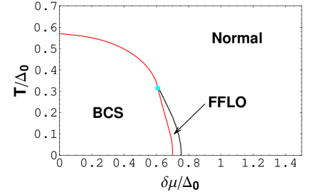
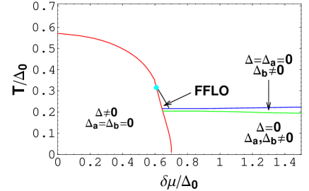
Refer to caption
Refer to caption
Figure 1: (color online) The phase diagram in $T-\delta\mu$ plane at fixed $\mu=50\Delta_{0}$ with $\Delta_{0}$ being the symmetric gap at $\delta\mu=0$. The upper panel is with only double-species pairing, and in the bottom panel the single-species pairing is included as well.

The phase diagram in $T-\delta\mu$ plane is shown in Fig.1. The upper panel is in the familiar case without single-species pairing[32]. The homogeneous BCS state can exist at low temperature and low mismatch, and the inhomogeneous FFLO state survives only in a narrow mismatch window. When the single-species pairing is included as well, see the bottom panel of Fig.1, the inhomogeneous FFLO state of $a$-$b$ pairing is eaten up by the homogeneous superfluid of $a$-$a$ and $b$-$b$ pairings at low temperature, just as we expected, and survives only in a small triangle at high temperature. The phase transition from the $a$-$b$ pairing superfluid to the $a$-$a$ and $b$-$b$ pairing superfluid is of first order. Note that for systems with fixed chemical potentials there is no mixed phase of double- and single-species pairings, and the situation is similar to a three-component fermion system[33].

4 Summary

We have investigated the phase structure of an asymmetric two-species fermion superfluid with both double- and single-species pairings. Since the attractive interaction for the single-species pairing is relatively weaker, it changes the conventional phase diagram at low temperature. In any system with chemical potential imbalance, the double-species pairing in FFLO state is replaced by the single-species pairing. In the region with single-species pairing, the interesting gapless superfluid is washed out and all fermion excitations are fully gapped. We should note that in this paper we considered only the grand canonical ensemble. For the case of canonical ensemble, the phase diagram becomes much more rich[22].

Acknowledgments: The work was supported by the grants NSFC10575058, 10425810 and 10435080.

References

  • [1] M.W.Zwierlein $et\,\ al.$, Science 311, 492(2006).
  • [2] G.B.Partidge $et\,\ al.$, Science 311, 503(2006).
  • [3] Y.Shin $et\,\ al.$, Phys. Rev. Lett. 97, 030401(2006).
  • [4] D.T.Son and M.A.Stephanov, Phys. Rev. A74, 013614(2006).
  • [5] J.Carlson and S.Reddy, Phys. Rev. Lett. 95, 060401(2005).
  • [6] L.He, M.Jin and P.Zhuang, Phys. Rev. B73, 214527(2006).
  • [7] M.Iskin and C.A.R.Sa de Melo, Phys. Rev. B74, 144517(2006); Phys. Rev. Lett. 97, 100404(2006).
  • [8] A.Bulgac, M.M.Forbes and A.Schwenk, Phys. Rev. Lett. 97, 020402(2006).
  • [9] T.Ho and H.Zhai, cond-mat/0602568.
  • [10] I.Giannakis, D.Hou, M.Huang and H.Ren, cond-mat/0603263.
  • [11] H.Hu and X.Liu, Phys. Rev. A73, 051603(R)(2006).
  • [12] K.Machida, T.Mizushima and M.Ichioka, Phys. Rev. Lett. 97, 120407(2006).
  • [13] H.Caldas, cond-mat/0605005.
  • [14] G.Sarma, J.Phys.Chem.Solids 24, 1029(1963).
  • [15] I.Shovkovy and M.Huang, Phys. Lett. B564, 205(2003);M.Huang and I.Shovkovy, Phys.Rev.D 70, 094030(2004).
  • [16] W.Liu and F.Wilczek, Phys. Rev. Lett. 90, 047002(2003).
  • [17] P.Fulde and R.Ferrel, Phys. Rev. A135,550(1964); A.Larkin and Y.Ovchinnikov, Sov. Phys. JETP 20,762(1965).
  • [18] H.Muther and A.Sedrakian, Phys. Rev. Lett. 88, 252503(2002).
  • [19] A.Sedrakian $et\,\ al.$, Phys. Rev. A72, 013613(2005).
  • [20] P.Bedaque, H.Caldas and G.Rupak, Phys. Rev. Lett. 91, 247002(2003).
  • [21] H.Caldas, Phys. Rev. A69, 063602(2004).
  • [22] X.Huang,X.Hao and P.Zhuang, New J. Phys. 9,375 (2007), [arXiv: cond-mat/0610610].
  • [23] M.Huang, P.Zhuang and W.Chao, Phys. Rev. D67, 065015(2003); I.Shovkovy, Found. Phys. 35, 1309(2005); M.Huang, Int.J.Mod.Phys.E14, 675(2005); H.Ren, hep-ph/0404074.
  • [24] U.Lombardo $et\,\ al.$, Int.J.Mod.Phys. E14,513(2005).
  • [25] M.Iavarone $et\,\ al.$, Phys. Rev. Lett. 89, 187002(2001).
  • [26] F.Bouquet $et\,\ al.$, Phys. Rev. Lett. 89, 257001(2002).
  • [27] S.Tsuda $et\,\ al.$, Phys. Rev. Lett. 91, 127001(2003).
  • [28] J.Geerk $et\,\ al.$, Phys. Rev. Lett. 94, 227005(2005).
  • [29] I.M.Khalatnikov, JETP Lett. 17, 386(1973).
  • [30] V.p.Mineev, Sov. Phys.JETP 40, 132(1974).
  • [31] Y.A.Nepomnyashchii, Theor. Math. Phys. 20, 904(1974); Sov. Phys. JETP 43, 559(1976).
  • [32] S.Takata and T.Izuyama, Prog. Theor. Phys. 41, 635(1969).
  • [33] T.Paananen, J.Martikainen and P.Torma, Phys. Rev. A73, 053606(2006).