Spontaneous creation of chromomagnetic field and $A_{0}$-condensate at high temperature on a lattice

Abstract

In a lattice formulation of $SU(2)$-gluodynamics, the spontaneous generation of chromomagnetic fields at high temperature is investigated. A procedure to determine this phenomenon is developed. By means of the $\chi^{2}$-analysis of the data set accumulating $5-10\times 10^{6}$ Monte Carlo configurations, the spontaneous creation of the Abelian color magnetic field is indicated. The common generation of the magnetic field and $A_{0}$-condensate is also studied. It is discovered that the field configuration consisting of the magnetized vacuum and the $A_{0}$-condensate is stable.

1 Introduction

Nowadays it is generally accepted that the non-linearity of non-Abelian gauge fields could result in formation of field condensates. The first model of gluon condensate, so called ”color ferromagnetic vacuum state”, was proposed thirty years ago by Savvidy [1]. It describes the spontaneous generation of the uniform Abelian chromomagnetic field $H=const$ due to a vacuum polarization. Unfortunately, this state is unstable because of the tachyonic mode in the gluon spectrum [2, 3]. This situation is changed at finite temperature when the spectrum stabilization happens due to either a gluon magnetic mass [6] or a so-called $A_{0}$-condensate [5] that is implemented in a stable magnetized vacuum. These are the extensions of the Savvidy model to the finite temperature case investigated already by the methods of continuum field theory [4, 5, 6]. In these ways the possibility of the spontaneous generation of strong temperature-dependent and stable color magnetic fields of order $gH\sim g^{4}T^{2}$, where $g$ is a gauge coupling constant, $T$ - temperature, is realized. The field stabilization is ensured by the temperature and field dependent gluon magnetic mass, which serves as a regulator of infrared singularities at $T\not=0$.

Such spontaneously created ”primordial” color magnetic fields had been generated at a GUT scale [7]. They could serve as seed fields responsible for generation of the large-scale magnetic fields detected in astrophysical observations [8]. The presence of strong magnetic fields in the early universe is of paramount importance for its evolution. In particular, a present day cosmic magnetic field of order $B_{0}\sim(4-5)\times 10^{-9}G$ could produce the recently discovered Wilkinson Microscopic Anisotropy Probe (WMAP) anomaly [9].

In Refs. [6, 10] the spontaneous creation of the chromomagnetic fields was observed in $SU(2)$- and $SU(3)$-gluodynamics within the one-loop plus daisy resummations. In Ref. [11] the chromomagnetic condensate of the same order was calculated in a stochastic QCD vacuum model by comparison with some data of lattice simulations. In Ref. [12] the spontaneous generation of the chromomagnetic field at high temperature was investigated in a lattice formulation of $SU(2)$-gluodynamics. In Refs. [13] the response of the vacuum to the influence of strong external fields at different temperatures was investigated and it has been shown that confinement is restored when the strength of the external field is increased.

Other condensate, which formation at $T\not=0$ was investigated in continuum field theory [14], is the zero component of the gluon electrostatic potential $A_{0}=const$. It acts to stabilize the QCD vacuum magnetized state, as it was discussed in Ref. [5]. In this paper, however, the magnetic field was considered as external one. Whether or not the actual value of the $A_{0}$ generated in the deconfining phase is sufficient to remove the tachyonic instability was not estimated.

The main goal of present paper is to investigate the common generation of the chromomagnetic field and $A_{0}$-condensate in lattice simulations. To incorporate the chromomagnetic field on a lattice we use the method developed in [12]. Instead of the field strength, which is quantized, the magnetic fluxes are considered as the objects to be investigated. The flux takes continuous values. Therefore the minimization of free energy of the flux can be done in a usual known procedure. The values of the strength of spontaneously generated magnetic field and the values of the Polyakov loop for corresponding states were obtained from Monte Carlo (MC) simulations. Then the value of $A_{0}$ was derived by using a procedure developed in Ref.[15].

The paper is organized as follows. In section 2, necessary information about the chromomagnetic fluxes on a lattice is educed and the results of calculations are given. In section 3, the investigation of the effect of combined generation of chromomagnetic field and $A_{0}$-condensate is presented. The final section is devoted to discussion.

2 Chromomagnetic fields on a lattice

In continuum, to determine the spontaneous generation of a magnetic field one has to minimize the effective potential (or free energy) of the background field. The background field is introduced by splitting of the gauge field potential $A_{\mu}$ into the quantum $A_{\mu}^{R}$ and classical $\bar{A_{\mu}}$ parts: $A_{\mu}=A_{\mu}^{R}+\bar{A_{\mu}}$. We choice the potential $\bar{A_{\mu}}^{a}=(0,0,Hx^{1},0)\delta^{a3}$ that corresponds to a constant chromomagnetic field directed along the third axis in the Euclidean and color space.

We relate the free energy density of the flux to the effective action according to the definition,

$$F(\varphi)=\bar{S}(\varphi)-\bar{S}(0),$$ (1)

where $\bar{S}(\varphi)$ and $\bar{S}(0)$ are the effective lattice actions with and without chromomagnetic field, correspondingly, $\varphi$ is the field flux.

To detect the spontaneous creation of the field it is necessary to show that free energy has a global minimum at non-zero flux, $\varphi_{min}\not=0$.

In what follows, we use the hypercubic lattice $L_{t}\times L_{s}^{3}$ ($L_{t}<L_{s}$) with the hypertorus geometry; $L_{t}$ and $L_{s}$ are the temporal and the spatial sizes of the lattice, respectively. In the limit of $L_{s}\to\infty$ the temporal size $L_{t}$ is related to physical temperature. The standard Wilson action of the $SU(2)$ lattice gauge theory can be written as

$$S_{W}=\beta\sum_{x}\sum_{\mu>\nu}\left[1-\frac{1}{2}\Tr U_{\mu\nu}(x)\right];$$ (2)

$$U_{\mu\nu}(x)=U_{\mu}(x)U_{\nu}(x+a\hat{\mu})U_{\mu}^{\dagger}(x+a\hat{\nu})U_{\nu}^{\dagger}(x),$$ (3)

where $\beta=4/g^{2}$ is the lattice coupling constant, $g$ is the bare coupling, $U_{\mu}(x)$ is the link variable located on the link leaving the lattice site $x$ in the $\mu$ direction, $U_{\mu\nu}(x)$ is the ordered product of the link variables. The effective action $\bar{S}$ in (1) is the Wilson action $S_{W}$ averaged over the Boltzmann configurations produced in the MC simulations.

The lattice variable $U_{\mu}(x)$ can be decomposed in terms of the unity, $I$, and Pauli, $\sigma_{j},$ matrices in the color space,

$$U_{\mu}(x)=IU_{\mu}^{0}(x)+i\sigma_{j}U_{\mu}^{j}(x).$$ (4)

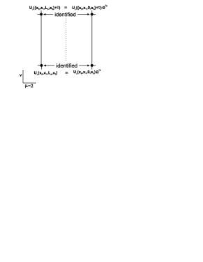
Figure 1: The plaquette presentation of the twisted boundary conditions.

The chromomagnetic flux $\varphi$ through the whole lattice was introduced by applying the twisted boundary conditions [16] (Fig. 1). In this approach the edge links in all directions are identified as usual periodic boundary conditions except for the links in the second spatial direction, for which the additional phase $\varphi$ is added. The magnetic flux $\varphi$ is measured in angular units and can take a value from $0$ to $2\pi$.

The twisted boundary conditions (t.b.c.) for the components of (4) are

$$U^{0}_{\mu}(x)\leftrightarrow\Biggl{\{}\begin{array}[]{l}U^{0}_{\mu}\cos\varphi-U^{3}_{\mu}\sin\varphi~{}~{}~{}~{}$for$~{}x=\{x_{0},x_{1},L_{s},x_{3}\}~{}$and$~{}\mu=2,\\ U^{0}_{\mu}\hskip 108.12054pt~{}$for other links$,\end{array}$$ (7)

$$U^{3}_{\mu}(x)\leftrightarrow\Biggl{\{}\begin{array}[]{l}U^{0}_{\mu}\sin\varphi+U^{3}_{\mu}\cos\varphi~{}~{}~{}~{}$for$~{}x=\{x_{0},x_{1},L_{s},x_{3}\}~{}$and$~{}\mu=2,\\ U^{3}_{\mu}\hskip 108.12054pt~{}$for other links$.\end{array}$$ (10)

The relations (7) and (10) have been implemented into the kernel of the MC procedure in order to produce the configurations with the chromomagnetic flux $\varphi$. Thus, the flux $\varphi$ is taken into account while obtaining a Boltzmann ensemble at each MC iteration.

The MC simulations are carried out by means of the heat bath method. The lattices $2\times 8^{3}$, $2\times 16^{3}$ and $4\times 8^{3}$ at $\beta=3.0$, $5.0$ are considered. These values of the coupling constant correspond to the deconfinement phase and perturbative regime. To thermalize the system, 200-500 iterations are fulfilled. At each working iteration, the plaquette value (3) is averaged over the whole lattice leading to the Wilson action (2). Then the effective action is calculated by averaging over the 1000-5000 working iterations. By setting a set of chromomagnetic fluxes $\varphi$ in the MC simulations we obtain the corresponding set of values of the effective action. The value of the condensed chromomagnetic flux $\varphi_{min}$ is obtained as the result of minimization of the free energy density (1) in the $\varphi$.

The spontaneous generation of chromomagnetic field is the effect of order $\sim g^{4}$ [6]. The results of MC simulations show the comparably large dispersion. So, the large amount of the MC data is collected and the standard $\chi^{2}$-method for the analysis of data is applied to determine the effect. We consider the results of the MC simulations as observed “experimental data”.

The effective action depends smoothly on the flux $\varphi$ in the region $\varphi\sim 0$. So, the free energy density can be fitted by a quadratic function of $\varphi$,

$$F(\varphi)=F_{min}+b(\varphi-\varphi_{min})^{2}.$$ (11)

In Eq.(11 ), there are three unknown parameters, $F_{min}$, $b$ and $\varphi_{min}$. $\varphi_{min}$ denotes the minimum position of free energy, whereas the $F_{min}$ and $b$ are the free energy density at the minimum and the curvature of the free energy function, correspondingly.

The value $\varphi_{min}$ is obtained as a result of minimization of the $\chi^{2}$-function

$$\chi^{2}(F_{min},b,\varphi_{min})=\sum_{i}\frac{(F_{min}+b(\varphi_{i}-\varphi_{min})^{2}-F(\varphi_{i}))^{2}}{D(F(\varphi_{i}))},$$ (12)

$$D(F(\varphi_{i}))=\sum_{i\in bin}\frac{(F(\varphi_{i})-\hat{F}_{bin})^{2}}{n_{bin}-1},$$ (13)

where $\varphi_{i}$ is the array of the set of fluxes and $D(F(\varphi_{i}))$ is the data dispersion, which can be obtained by collecting the data into bins (as a function of $\varphi$); $n_{bin}$ is a number of points and and $\hat{F}_{bin}$ is a mean value of free energy density in the considered bin. As it was determined in the data analysis, the dispersion is independent of $\varphi$. The deviation of $\varphi_{min}$ from zero indicates the presence of the spontaneously generated field.

Table 1: The values of the generated fluxes $\varphi_{min}$ for different lattices.

	$2\times 8^{3}$	$2\times 16^{3}$	$4\times 8^{3}$
$\beta=3.0$	${0.019^{+0.013}_{-0.012}}$	$0.0069^{+0.0022}_{-0.0057}$	$0.005^{+0.005}_{-0.003}$
$\beta=5.0$	${0.020^{+0.011}_{-0.010}}$

The fit results are given in the Table 1. As one can see, $\varphi_{min}$ demonstrates the $2\sigma$-deviation from zero.

The 95% C.L. domain of parameters $F_{min}$ ($b$ for the right figure) and $\varphi_{min}$ is represented in Fig. 2. The black cross marks the position of the maximum-likelihood values of $F_{min}$ ($b$ for the right figure) and $\varphi_{min}$. It can be seen that the flux is positively determined. The 95% C.L. area becomes more symmetric with the center at the $F_{min}$, $b$ and $\varphi_{min}$ when the statistics is increased. This also confirms the results of the carried out fitting.

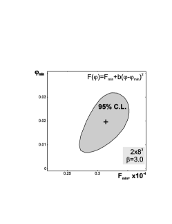
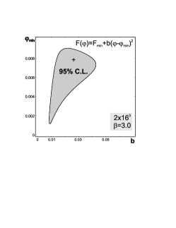
Figure 2: The 95% C.L. area for the parameters $F_{min}$ and $\varphi_{min}$, determining the free energy density dependence on the flux $\varphi_{min}$ on lattice $2\times 8^{3}$ for $\beta=3.0$ (left figure). The 95% C.L. area for the parameters $F_{min}$ and $b$ , determining the free energy density dependence on the flux $\varphi_{min}$ on lattice $2\times 16^{3}$ for $\beta=3.0$ (right figure).

3 The spontaneous vacuum magnetization and $A_{0}$-condensate

In this section we investigate an effective potential, taking into consideration the effects of non-trivial $A_{0}$-condensate and chromomagnetic field [15]. This is realized by means of calculation of the partition function in a general covariant background field gauge with the background field providing both the chromomagnetic field and the non-trivial Polyakov loop. Then the data obtained in MC simulations are substituted in this effective potential. If the minimum value of it is negative and the potential is real, the common generation of condensates happens.

Within the used imaginary time formalism, the temporal direction in the Eucleadian space is periodic, with period $\beta=1/T$, and the Polyakov loop $P_{L}$, defined as the time-ordered exponential,

$$P_{L}(\vec{x})=T\exp\left[ig\oint d\tau A_{0}(\vec{x},\tau)\right],$$ (14)

is a proper order parameter to describe the deconfinement phase transition. It is specified by a constant $A_{0}$ field, given in the fundamental representation by

$$A_{0}=\frac{\phi}{g\beta}\frac{\tau_{3}}{2},$$ (15)

where $0\leq\phi\leq 2\pi$, $\tau_{3}$ is Pauli matrix.

The trace of the Polyakov loop in the fundamental representation is

$$\Tr_{F}(P_{L})=2\cos(\phi/2).$$ (16)

Unless the $Z(2)$symmetry is spontaneously broken, the variable $\phi$ has to have the value $\pi$ corresponding to $\Tr_{F}(P_{L})=0$.

The one-loop contribution to the free energy has the form [15]

$$V^{(1)} = V^{(1)}_{0}+V^{(1)}_{\pm}$$

$$= \sum_{n}\frac{1}{\beta}\int\frac{d^{3}\vec{k}}{(2\pi)^{3}}\log(\omega_{n}^{2}+\vec{k}^{2})+$$

$$\frac{1}{2}\sum_{m=0}^{\infty}\sum_{n,\pm}\frac{1}{\beta}\frac{gH}{2\pi}\int\frac{dk_{3}}{2\pi}\log\left[(\omega_{n}-\frac{\phi}{\beta})^{2}+2gH(m+\frac{1}{2}\pm 1)+k_{3}^{2}\right]+$$

$$\frac{1}{2}\sum_{m=0}^{\infty}\sum_{n,\pm}\frac{1}{\beta}\frac{gH}{2\pi}\int\frac{dk_{3}}{2\pi}\log\left[(\omega_{n}+\frac{\phi}{\beta})^{2}+2gH(m+\frac{1}{2}\pm 1)+k_{3}^{2}\right],$$

where $\omega_{n}=2\pi n/\beta$ is the Matsubara frequency, and the sum over $n$ is over all integer values. The sum over $m$ is the sum over the Landau levels.

By applying a standard technique of Schwinger to express the logarithms of (3) as an integral and performing the high-temperature expansion of the effective potential, we obtain

$$V^{(1)}=C_{1}\frac{(gH)^{2}}{8\pi^{2}}-\frac{(gH)^{3/2}}{4\pi^{3/2}\beta}\sum^{\infty}_{k=2}\frac{2^{2k}B_{2k}}{(2k)!}\Gamma(2k-3/2)\times$$ (18)

$$\sum_{l}\left(\frac{\beta^{2}gH}{\beta^{2}gH+(\phi-2\pi l)^{2}}\right)^{2k-3/2}+\frac{(gH)^{2}}{24\pi^{2}}(3-4\gamma)-\frac{2\pi^{2}}{45\beta^{4}}$$

$$+\frac{\phi^{2}}{3\beta^{4}}+\frac{\phi^{4}}{12\pi^{2}\beta^{4}}+\frac{gH}{2\pi\beta^{2}}\sqrt{-gH\beta^{2}+\phi^{2}}+\frac{g^{2}H^{2}}{12\pi\sqrt{gH\beta^{2}+\phi^{2}}}$$

$$-\frac{(gH\beta^{2}+\phi^{2})^{3/2}}{3\pi\beta^{2}}-\frac{g^{2}H^{2}\log\left[\frac{\sqrt{-gH}\beta}{4\pi}\right]}{4\pi^{2}}+\frac{g^{2}H^{2}\log\left[\frac{\sqrt{gH}\beta}{4\pi}\right]}{12\pi^{2}}$$

$$-\frac{g^{2}H^{2}\phi^{2}\zeta[3]}{24\pi^{4}}-\frac{g^{3}H^{3}\beta^{2}\zeta\left[3,-\frac{\phi}{2\pi}\right]}{192\pi^{4}}-\frac{g^{3}H^{3}\beta^{2}\zeta\left[3,\frac{\phi}{2\pi}\right]}{192\pi^{4}}+O(\beta^{2}(gH)^{3}).$$

Here $C_{1}=-0.01646$, $\gamma\simeq 0.577216$ is Euller’s constant, $\zeta(s)$ is the Riemann Zeta-function, $B_{n}$ are the Bernoulli numbers.

We performed the described above lattice calculations and have obtained the values for the spontaneously generated field strength and the Polyakov loop of corresponding states. Then we considered the expression (18) as a function of these parameters and studied its minimum. We have determined that for the temperatures $1/\beta=100-500GeV$, the field strengths $H=10^{22}-10^{24}G$, and $\phi=2.0-3.11$ the one-loop effective potential (18) is negative, $V^{(1)}(H,\phi,\beta)<0$. Hence it follows, either gauge field or $A_{0}$ condensate are spontaneously generated. Moreover, in the minimum of the effective potential for used values of the parameters the ratio $ImV^{(1)}/ReV^{(1)}$ is of order $\sim 10^{-10}$, that is practically zero for numeric calculations. We conclude that the common generation of the constant Abelian chromomagnetic field and the non-trivial Polyakov loop results in the stable magnetized vacuum state. Of course, the one-loop potential does not exhibit the complete effective potential. However, it gives the main contribution which contains a larger imaginary part. If one adds the second next-to-leading contribution coming from ring diagrams, this part is cancelled [6]. So, the check of stabilization at one-loop level is important.

4 Discussion

We have investigated the effect on common spontaneous generation of chromomagnetic field and $A_{0}$-condensate in $SU(2)$-gluodynamics at high temperature. The first step was to show the possibility of the spontaneous generation of chromomagnetic field at high temperature [12]. The obtained results are in a good agreement with that of derived already in the continuum quantum field theory [6, 17] and in the lattice data analysis [11]. The actual values of the chrmomomagnetic field strength and the Polyakov loop were obtained from the same MC simulations. They allow to conclude that these condensates, chromomagnetic field and $A_{0}$, have to be present in the deconfinement phase of QCD.

The developed approach joins the calculation of free energy functional $F(\phi)$ and the consequent statistical analysis of its minimum positions for various temperatures and flux values. In this way the spontaneous creation of condensates is realized in lattice simulations.

Other important result of the present work is that the spontaneously magnetized state is stable. This indicates that a true vacuum at high temperature is formed from these condensates.

Since the field configuration with constant fields is gauge non-invariant, one could consider this configuration as a domain. A complete structure of whole space can be derived by using the requirement of gauge invariance for the space including domains with different orientation. This problem we left for the future.

We would like to conclude that in the deconfinement phase the condensates have to influence various processes that should be taken into consideration to have an adequate concept about this state.

References

References

- [1] G.K. Savvidy, Phys. Lett. B 71, 133 (1977).
- [2] V.V. Skalozub, Yadernaya Fizika 28, 228 (1978).
- [3] N.K. Niesen, P. Olesen, Nucl. Phys. B 144 , 376 (1978).
- [4] K. Enqvist, P. Olesen, Phys. Lett. B 329, 195 (1994).
- [5] A. Starinets, A. Vshivtsev, V. Zhukovsky, Phys. Lett. B 322, 403 (1994).
- [6] V. Skalozub, M. Bordag, Nucl. Phys. B 576, 430 (2000).
- [7] M. Pollock, Int. J. Mod. Phys. D 12, 1289 (2003).
- [8] D. Grasso, H. Rubinstein, Phys. Rept. 348, 163 (2001).
- [9] L. Campanelli, P. Cea, L. Tedesco, Phys. Rev. Letters 97, 131302 (2006).
- [10] V. Skalozub, A. Strelchenko, Eur. Phys. J. C 40, 121 (2005).
- [11] N. Agasian, Phys. Lett. B 562, 257 (2003).
- [12] V. Demchik, V. Skalozub, to be published in Yad.Fiz. 1(2008), hep-lat/0601035.
- [13] P. Cea, L. Cosmai, Phys. Rev. D 60, 094506 (1999); JHEP 0508, 079 (2005); hep-lat/0101017.
-
[14]
K. Enqvist, K. Kajantie,
Z. Phys. C 47, 291 (1990);
D. Ebert, V.Ch. Zhukovsky, A.S. Vshivtsev, Int. J. Mod. Phys. A 13, 1723 (1998);
O. Borisenko, J. Bohacik, V. Skalozub, Fortsch. Phys. 43, 301 (1995). - [15] P. Meisinger, M. Ogilvie, Phys. Rev. D 66, 105006 (2002).
- [16] G.’t Hooft, Nucl. Phys. B 153, 141 (1979).
- [17] V. Skalozub, A. Strelchenko, Eur. Phys. J. C 33, 105 (2004).