Dynamic 3-Coloring of Claw-free Graphs

Abstract

A dynamic $k$-coloring of a graph $G$ is a proper $k$-coloring of the vertices of $G$ such that every vertex of degree at least 2 in $G$ will be adjacent to vertices with at least 2 different colors. The smallest number $k$ for which a graph $G$ can have a dynamic $k$-coloring is the dynamic chromatic number, denoted by $\chi_{d}(G)$. In this paper, we investigate the dynamic 3-colorings of claw-free graphs. First, we prove that it is $NP$-complete to determine if a claw-free graph with maximum degree 3 is dynamically 3-colorable. Second, by forbidding a kind of subgraphs, we find a reasonable subclass of claw-free graphs with maximum degree 3, for which the dynamically 3-colorable problem can be solved in linear time. Third, we give a linear time algorithm to recognize this subclass of graphs, and a linear time algorithm to determine whether it is dynamically 3-colorable. We also give a linear time algorithm to color the graphs in the subclass by 3 colors.
Keywords: Claw-free graph; Vertex coloring; Dynamic coloring; (Dynamic) Chromatic number; $NP$-complete; Linear time algorithm

1 Introduction

We follow the terminology and notations of [1] and, without loss of generality, consider simple connected graphs only. $\delta(G)$ and $\Delta(G)$ denote, respectively, the minimum and maximum degree of a graph $G$. For a vertex $v\in V(G)$, the neighborhood of $v$ in $G$ is $N_{G}(v)=\{u\in V(G):u$ is adjacent to $v$ in $G\}$, and the degree of $v$ is $d(v)=|N_{G}(v)|$. Vertices in $N_{G}(v)$ are called neighbors of $v$. $P_{n}$ denotes the path on $n$ vertices. A subset $S$ of $V$ is called an independent set of $G$ if no two vertices of $S$ are adjacent in $G$. An independent set $S$ is maximum if $G$ has no independent set $S^{\prime}$ with $|S^{\prime}|>|S|$. The number of vertices in a maximum independent set of $G$ is called the independence number of $G$ and is denoted by $\alpha(G)$.

For an integer $k>0$. A proper $k$-coloring of a graph $G$ is a surjective mapping $c:\ V(G)\rightarrow\{1,2,\ldots,k\}$ such that if $u,v$ are adjacent vertices in $G$, then $c(u)\neq c(v)$. The smallest $k$ such that $G$ has a proper $k$-coloring is the chromatic number of $G$, denoted by $\chi(G)$.

The dynamic coloring of a graph $G$ is defined as a proper coloring of $G$ such that any vertex of degree at least 2 in $G$ is adjacent to more than one color class. For an integer $k>0$, a proper dynamic $k$-coloring of a graph $G$ is thus a surjective mapping $c:V(G)\rightarrow\{1,2,\ldots,k\}$ such that both of the following two conditions hold:

• if $u,v\in V(G)$ are adjacent vertices in $G$, then $c(u)\neq c(v)$; and

• for any $v\in V(G)$, $|c(N_{G}(v))|\geq min\{d(v),2\}$, where and in what follows, $c(S)=\{c(u)|u\in S$ for a set $S\subseteq V(G)\}$.

We call the first condition, which characters proper coloring, the adjacency condition, and we call the second condition the double-adjacency condition. The smallest integer $k>0$ such that $G$ has a proper dynamic $k$-coloring is the dynamic chromatic number of $G$, denoted by $\chi_{d}(G)$.

In order to show the results in this paper, we will give some new definitions. Similar to the definition of the dynamic coloring, a dynamic $k$-edge-coloring of a graph $G$ is a proper $k$-edge-coloring of $G$ such that every edge with at least 2 adjacent edges in $G$ will be adjacent to edges with at least two different colors. The smallest number $k$ for which a graph $G$ can have a dynamic $k$-edge-coloring is the dynamic edge chromatic number, denoted by ${\chi_{d}}^{\prime}(G)$.

The dynamic chromatic number has very different behaviors from the traditional chromatic number. For example, from [4] we know that for many graphs $G$, $\chi_{d}(G-v)>\chi_{d}(G)$ for at least one vertex $v$ of $G$, and there are graphs $G$ for which $\chi_{d}(G)-\chi(G)$ may be very large.

From [3] we know that if $\Delta(G)\leq 2$, we can easily have a polynomial time algorithm to give the graph $G$ a dynamic $\chi_{d}$-coloring. In [2], Lai, Montgomery and Poon got an upper bound of $\chi_{d}(G)$ that if $\Delta(G)\geq 3$, then $\chi_{2}(G)\leq\Delta(G)+1$. The proof is very long compared with the proof of a similar result in the traditional coloring. In [3] and [4], Lai, Lin, Montgomery, Shui and Fan got many new and interesting results on the dynamic coloring. Recently, in [5] we proved that it is $NP$-complete to determine if a triangle-free graph with maximum degree 3 is dynamically 3-colorable. This is a little interesting because we know that for graphs $G$ with $\Delta(G)=3$ the $3$-colorable problem of the traditional vertex coloring can be solved in polynomial time.

Let $G$ be a graph with maximum degree 3. We define a family of subgraphs $A_{i}$ of $G$, in which every $A_{i}$ is a path with $i$ vertices such that the $i-2$ internal vertices have degree 2 in $G$, and the two end-vertices have degree 3 in $G$. A pendant path of a graph $G$ is such a path that the internal vertices have degree 2 in $G$, one end-vertex has degree 1 and the other end-vertex has degree 3. In the present paper, we concentrate on the dynamically 3-colorable problem for claw-free graphs. First, we prove that for a claw-free graph $G$ with $\Delta(G)=3$ it is still $NP$-complete to decide if $G$ is dynamically 3-colorable. This is also an interesting result which is different from a result for the traditional colorings. In order to find some kind of graphs for which the dynamically 3-colorable problem is polynomially solvable, we consider the subclass of the claw-free graphs with maximum degree 3, in which every graph is $A_{i}$-free $(i=3j+1,\ j\in\mathbb{Z}^{+})$. We find that this kind of graphs can be recognized in $O(n)$ time, and it can be done in $O(n)$ time to determine whether they are dynamically 3-colorable, and we will give an $O(n)$ time algorithm to find a dynamic 3-coloring of the graphs.

2 $NP$-complete results

In [3], the authors proved the following theorem:

Theorem 2.1

If $G$ is claw-free, then $\chi_{d}(G)\leq\chi(G)+2$, and the equality holds if and only if $G$ is a cycle of length 5 or of even length not a multiple of 3.

So, apart from some special cycles, the difference between the dynamic chromatic number and the chromatic number for claw-free graphs is at most one. If we know $\chi(G)$ and there would be a polynomial time algorithm to determine $\chi(G)=\chi_{d}(G)$ or $\chi(G)=\chi_{d}(G)+1$ except the special cycles described in Theorem 2.1, we can get some results on dynamic colorings by those on the traditional colorings for claw-free graphs. But unfortunately, we will show that even if we know the chromatic number of claw-free graphs, we cannot get the dynamic chromatic number in polynomial time unless $P=NP$. By the relation between the edge-coloring of a graph $G$ and the vertex coloring of the line graph $L(G)$ of $G$, we will get the result immediately after we finish the proof of the following Theorem 2.2.

First, we give a formal definition of the dynamically 3-edge-colorable problem, denoted by Dy-3-Edge-Col, which is stated as follows:

Input: A bipartite graph $B=B(V,E)$ and $\Delta(B)=3$.

Question: Can one assign each edge a color, so that only 3 colors are used and this is a dynamic edge-coloring ? i.e., is ${\chi_{d}}^{\prime}(B)\leq 3$ ?

In [6], the author proved that it is $NP$-complete to determine whether a cubic graph is 3-edge-colorable. We will use the result to prove that the Dy-3-Edge-Col is $NP$-complete.

Theorem 2.2

The Dy-3-Edge-Col is $NP$-complete.

Proof.   First, it is obvious that the problem is in $NP$.

Second, given a cubic graph $C$. For every edge in $C$, we will use a $P_{5}$ to replace the edge and construct a new graph $B$, i.e., we subdivide every edge exact 3 times. The local transformation is shown in Figure 1.

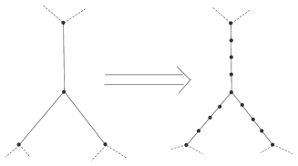
Figure 1: The local transformation

It is easy to see that $C$ is 3-edge-colorable if and only if $B$ is dynamically 3-edge-colorable. And, by the structure of $B$, the length of every cycle of $B$ is a multiple of 4. So $B$ does not have any odd cycles, and thus is a bipartite graph. It is obvious that $\Delta(B)=3$. Since the 3-edge-colorability for cubic graphs is $NP$-complete, the Dy-3-Edge-Col must be $NP$-complete.  

Remark. In the proof, we can subdivide each edge $3j$ times for some $j\in Z^{+}$, instead of 3 times, and the proof can still hold. Different edge could use different $j$. Therefore, we have the following stronger statement.

Theorem 2.3

It is $NP$-complete to determine whether a graph $G$ is dynamically 3-edge-colorable, obtained from a cubic graph $C$ by subdividing each edge of $C$ $3j$ times for some $j\in Z^{+}$.

For traditional edge-colorings, if a graph $G$ is bipartite, then $\chi^{\prime}(G)=\Delta(G)$ and there is a polynomial time algorithm to color it. So, Theorem 2.2 is different from the result for traditional edge-colorings.

Next, we give a formal definition of dynamically 3-colorable problem, denoted by Dy-3-Col, which is stated as follows:

Input: A graph $G=G(V,E)$.

Question: Can one assign each vertex a color, so that only 3 colors are used and this is a dynamic coloring ? i.e., is ${\chi_{d}}(G)\leq 3$ ?

By the structure of the bipartite graph $B$ in the proof of Theorem 2.2, we know that $L(B)$ is a line graph with maximum degree 3. Notice that a graph $G$ is dynamically $k$-edge-colorable if and only if the line graph $L(G)$ of $G$ is dynamically $k$-colorable. So, we have

Theorem 2.4

It is $NP$-complete to determine whether the line graph $L(B)$ with maximum degree 3 is dynamically 3-colorable. As a result, it is $NP$-complete to determine whether a line graph with maximum degree 3 is dynamically 3-colorable.

Since line graphs are claw-free graphs, then we have

Theorem 2.5

For claw-free graphs $G$ with $\Delta(G)=3$, the Dy-3-Col is $NP$-complete.

For traditional colorings, it is polynomially solvable whether a graph $G$ is 3-colorable when $\Delta(G)\leq 3$. So we can see that the dynamic coloring problem is very difficult to deal with even for claw-free graphs with maximum degree 3. In next section we will find some reasonable kind of graphs in which we can determine if a graph is dynamically 3-colorable in polynomial time. Theorems 2.3 and 2.4 could be omitted as intermediate results. But, we prefer to list them in order to understand why we choose to study this kind of graphs in next section.

3 A polynomial time result

From Theorem 2.5, the Dy-3-Col is $NP$-complete for claw-free graphs with maximum degree 3, and because of Theorem 2.4, the problem is $NP$-complete even for the line graph $L(B)$, where $B$ is built up from a cubic graph by subdividing every edge exact 3 times. By reviewing the proof of Theorem 2.2, we notice that there are many $A_{4}$ in $L(B)$. The question is: can the Dy-3-Col be solved in polynomial time for both claw-free and $A_{4}$-free graphs $G$ with $\Delta(G)=3$ ? The answer is No, because in the local transformation, we can use any $P_{i}$ $(i=3j+2,\ j\in\mathbb{Z}^{+})$ to replace the edges of the cubic graph $C$ to get another graph $B^{\prime}$, and $C$ is 3-edge-colorable if and only if $B^{\prime}$ is dynamically 3-edge-colorable. Although $B^{\prime}$ may not be bipartite, we can still get Theorem 2.4. So, another question is: can the Dy-3-Col be solved in polynomial time for both claw-free and $A_{i}$-free (for all $i=3j+1,\ j\in\mathbb{Z}^{+}$) graphs $G$ with $\Delta(G)=3$ ? The answer is Yes. For convenience, we denote by $\mathscr{C}$ the set of graphs $G$ with $\Delta(G)\leq 3$ which are both claw-free and $A_{i}$-free $(i=3j+1,\ j\in\mathbb{Z}^{+})$. Then we have

Theorem 3.1

The Dy-3-Col is polynomially solvable for graphs in $\mathscr{C}$.

Proof.   Given a graph $G$ in $\mathscr{C}$. First, delete all the vertices in the pendant paths of $G$ except the end-vertices of degree 3, to get the first graph $G_{1}$. It is easy to see that $G$ is dynamically 3-colorable if and only if $G_{1}$ is dynamically 3-colorable. Then $G_{1}$ has vertices of only degrees 2 and 3. Second, delete all the internal vertices in $A_{i}$ $(i=3j+2,\ j\in\mathbb{Z}^{+})$ of $G_{1}$, and make the two end-vertices of each $A_{i}$ $(i=3j+2,\ j\in\mathbb{Z}^{+})$ be adjacent, to get the second graph $G_{2}$. It is easy to see that $G_{1}$ is dynamically 3-colorable if and only if $G_{2}$ is dynamically 3-colorable. Third, delete all the internal vertices in $A_{i}$ $(i=3j+3,\ j\in\mathbb{Z}^{+})$ of $G_{2}$, and make the two end-vertices of each $A_{i}$ $(i=3j+3,\ j\in\mathbb{Z}^{+})$ be adjacent, to get the third graph $G_{3}$. It is easy to see that $G_{2}$ is dynamically 3-colorable if and only if $G_{3}$ is dynamically 3-colorable. Fourth, consider the subgraphs $A_{3}$ in $G_{3}$, and there will be two kinds of $A_{3}$ in $G_{3}$: one kind is denoted by $A_{3}^{1}$, in which the two end-vertices of $A_{3}$ is adjacent (it means that the internal vertex is contained in a triangle), the other kind is denoted by $A_{3}^{2}$, in which the two end-vertices of $A_{3}$ is nonadjacent (it means that the internal vertex is not contained in a triangle). We delete all the internal vertices in $A_{3}^{2}$ of $G_{3}$, and make the two end-vertices of each $A_{3}^{2}$ be adjacent, to get the fourth graph $G_{4}$. It is easy to see that $G_{3}$ is dynamically 3-colorable if and only if $G_{4}$ is dynamically 3-colorable. By noticing that in $G_{4}$ every vertex is contained in a triangle, we have that $G_{4}$ is dynamically 3-colorable if and only if $G_{4}$ is 3-colorable. As a consequence, $G$ is dynamically 3-colorable if and only if $G_{4}$ is 3-colorable, and it is polynomially solvable whether $G_{4}$ is 3-colorable since $\Delta(G_{4})=3$. Because we can get $G_{4}$ from $G$ in polynomial time, the Dy-3-Col is polynomially solvable when $G$ is in $\mathscr{C}$.  

For traditional colorings, the only graph $G$ with $\Delta(G)\leq 3$ which is not 3-colorable is $K_{4}$ by Brook’s theorem. By the proof of Theorem 3.1 we can easily get that there is only one class of graphs in $\mathscr{C}$ which are not dynamically 3-colorable. The graphs in the exceptional class, denoted by $\mathscr{E}$, can be gotten by using a $P_{i}$ ($i=3j$ or $3j-1,\ j\in\mathbb{Z}^{+}$) to replace an edge of $K_{4}$.

For the graphs in $\mathscr{C}$ we can determine whether they are dynamically 3-colorable in polynomial time and we have also characterized the exceptional graphs.

In next section, we will give a linear time algorithm to recognize the graphs in $\mathscr{C}$ and another linear time algorithm to determine whether the graphs in $\mathscr{C}$ are dynamically 3-colorable. At last we will give a linear time algorithm to color the graphs by 3 colors such that the adjacency condition and the double-adjacency condition are both satisfied.

4 Linear time algorithms

First, we will give a linear time algorithm to recognize the graphs in $\mathscr{C}$. The input is a graph $G=G(V,E)$ with $|V|=n$. The following are the main steps of the recognition algorithm.

Algorithm 4.1 (Recognition Algorithm)

step 1.

Check if the degree of every vertex in $G$ is not more than 3. If not, return the answer that $G$ is not in $\mathscr{C}$; otherwise, go to step 2.

step 2.

Check if the graph $G$ is claw-free. If not, return the answer that $G$ is not in $\mathscr{C}$; otherwise, go to step 3.

step 3.

Check if the graph $G$ is $A_{i}$-free $(i=3j+1,\ j\in\mathbb{Z}^{+})$. If not, return the answer that $G$ is not in $\mathscr{C}$. Otherwise, return the answer that $G$ is in $\mathscr{C}$.

The following are the complexity analysis of the Recognition Algorithm: It is obvious that step 1 can be done in $O(n)$ time. If $\Delta(G)\leq 3$, we go to step 2, otherwise $G$ is not in $\mathscr{C}$. Since $\Delta(G)\leq 3$, we just need to check the vertices of degree 3. For every vertex of degree 3, if there is no claw in the subgraph induced by the vertex and its neighbors, $G$ is claw-free. So step 2 can be done in $O(n)$ time. If $G$ is claw-free, we go to step 3, otherwise $G$ is not in $\mathscr{C}$. In step 3, we just need to check the edges whose two incident vertices are of degree 2 in $G$. If the paths induced by the edges are not $P_{i}$ ($i=3j-1,\ j\in Z^{+}$), then $G$ is $A_{i}$-free $(i=3j+1,\ j\in\mathbb{Z}^{+})$. If $G$ is $A_{i}$-free $(i=3j+1,\ j\in\mathbb{Z}^{+})$, then $G$ is in $\mathscr{C}$, otherwise $G$ is not in $\mathscr{C}$. Since the number of edges in $G$ is no more than $\frac{3}{2}n$, step 3 can be done in $O(n)$ time.

Second, we give a linear time algorithm to determine if a graph in $\mathscr{C}$ is dynamically 3-colorable. The input is a graph $G=G(V,E)$ in $\mathscr{C}$ with $|V|=n$. The following are the main steps of the determination algorithm.

Algorithm 4.2 (Determination Algorithm)

step 1.

Check if there is a vertex of degree 1. If so, return the answer that $G$ is dynamically 3-colorable; otherwise, go to step 2.

step 2.

Find the number of vertices whose degrees are 3. If the number is not 4, return the answer that $G$ is dynamically 3-colorable; otherwise, go to step 3.

step 3.

Check if the graph $G$ is in $\mathscr{E}$. If so, return the answer that $G$ is not dynamically 3-colorable; otherwise, return the answer that $G$ is dynamically 3-colorable.

The following are the complexity analysis of the Determination Algorithm: It is easy to see that step 1 can be done in $O(n)$ time. If there is a vertex with degree 1, the graph $G$ is dynamically 3-colorable. If there is no vertex with degree 1, we go to step 2. Step 2 can also be done in $O(n)$ time. If the number of vertices of degree 3 is 4, we go to step 3. In step 3, we just need to consider the edges whose two incident vertices are of degree 2 in $G$. If there is no such edge, $G$ is dynamically 3-colorable if and only if $G$ is not $K_{4}$. If there are some such edges, we can determine if $G$ is dynamically 3-colorable by the subgraph induced by such edges. If there are more than one path in the subgraph, $G$ is dynamically 3-colorable. Otherwise, $G$ is in $\mathscr{E}$, and is not dynamically 3-colorable. Since the number of edges in $G$ is no more than $\frac{3}{2}n$, step 3 can be done in $O(n)$ time.

Third, we will give an $O(n)$ time algorithm to color the graphs in $\mathscr{C}$ by 3 colors such that the adjacency condition and the double-adjacency condition are both satisfied. The input is a graph $G=G(V,E)$ with $|V|=n$. Before we give the algorithm, we will define a set of graphs, denoted by $\mathscr{T}$, and give some results about the graphs in $\mathscr{T}$.

The graphs in $\mathscr{T}$ are constructed by the following two steps:

• Construct even number of vertex-disjoint triangles (3-cycles), and the set of edges in the triangles is denoted by $E_{1}(G)$;

• For each triangle, let every vertex of the triangle be connected by an edge to a vertex of another triangle, to construct a 3-regular graph. And the set of added edges in this step (it means that the set of the edges are not in any of the triangles) is denoted by $E_{2}(G)$.

Lemma 4.3

For any graph $G$ in $\mathscr{T}$, if there are $n$ triangles in $G$, then $\alpha(G)=n$.

Proof.   By the special structure of $G$ that every vertex is contained in a triangle, we can see that $\chi(G)=3$ and the three color classes have the same cardinality $n$. So, $\alpha(G)\geq n$. If $\alpha(G)>n$, there must be a triangle that contains 2 vertices in the maximum independent set, which is impossible, and so $\alpha(G)=n$.  

Lemma 4.4

Let $G$ be in $\mathscr{T}$ and there are $n$ triangles in $G$. For any maximum independent set $S$ of $G$, we have that $G\setminus S$ is bipartite.

Proof.   By Lemma 4.3, we know that $|S|=n$, and every triangle contains a vertex in $S$. So, in $G\setminus S$ the degrees of the vertices are 1 and 2. Then the components of $G\setminus S$ are only vertex-disjoint paths and cycles. Furthermore, no two edges in $E_{1}(G)$ are adjacent in $G\setminus S$. Also, no two edges in $E_{2}(G)$ are adjacent in $G\setminus S$. So, the cycles in $G\setminus S$ must be alternating and have even number of edges, i.e., there are no odd cycles in $G\setminus S$, and thus $G\setminus S$ is bipartite.  

Lemma 4.5

For any $G$ in $\mathscr{T}$, we can find a maximum independent set $S$ of $G$ in linear time.

Proof.   The algorithm is given as follows:

• We contract every triangle in $G$ into a vertex, and if there are two edges which are incident to the same two end-vertices, we can delete any one of the two edges, to get a simple graph $G^{\prime}$;

• By Depth-First or Breadth-First algorithm, we can find a spanning tree of a graph in $O(|V|+|E|)$ time. In our case, it is a linear time algorithm to find the spanning tree $T^{\prime}$ of $G^{\prime}$;

• Find a vertex $v_{r}$ which is adjacent to a leaf $v_{l}$ in $T^{\prime}$ as the root of the tree. If $d(v_{r})=3$, we delete $v_{l}$ to ensure $d(v_{r})=2$ in the new tree $T_{c}=T^{\prime}\setminus\{v_{l}\}$ we will consider later. If $d(v_{r})=2$, then $T_{c}$=$T^{\prime}$;

• For every edge $e_{c}$ in $T_{c}$, there are two vertices $v_{s}$ and $v_{f}$ incident to it, and $v_{s}$ is the child of $v_{f}$. By step (a), we know that there is an $e_{o}$ in $G$ corresponding to $e_{c}$ in $T_{c}$, and there is a vertex $v_{o}$ in the triangle corresponding to $v_{s}$ which is incident to $e_{o}$. So, we can define an injection $f$ from $E_{c}$, the set of edges in $T_{c}$, to $V(G)$ such that $f(e_{c})=v_{o}$. Then we can find a vertex set $f(E_{c})\subset V(G)$, and it is easy to see that $f(E_{c})$ is an independent set;

• Consider the three vertices in the triangle in $G$ corresponding to $v_{r}$, there is just one vertex $v_{r}^{o}$ of the three which can be added into $f(E_{c})$ such that $\{v_{r}^{o}\}\cup f(E_{c})$ is an independent set. If $d(v_{r})=2$ in $T^{\prime}$, then let $S=\{v_{r}^{o}\}\cup f(E_{c})$, which is a maximum independent set of $G$. If $d(v_{r})=3$, there is still a triangle in $G$ corresponding to $v_{l}$ in $T^{\prime}$ that needs us to consider. Notice that except the vertex in the triangle which is adjacent to $v_{r}^{o}$, any one of the other two vertices in the triangle (assume the vertex we choose is $v_{l}^{o}$) can be added into $\{v_{r}^{o}\}\cup f(E_{c})$ such that $S=\{v_{r}^{o},v_{l}^{o}\}\cup f(E_{c})$ is a maximum independent set of $G$.

One can easily see that the algorithm described above can be done in linear time. So we have proved the lemma.  

Now, it is time to give the dynamic 3-coloring algorithm for a given graph $G=G(V,E)\in\mathscr{C}$ with $|V|=n$. The following are the main steps of the algorithm.

Algorithm 4.6 (Dynamic 3-Coloring Algorithm)

step 1.

Delete all the pendant paths except the vertices with degree 3, to construct a graph $G_{1}$, if there are some pendant paths in $G$;

step 2.

If there are some $A_{i}$ ($i>3$) and $A_{3}$ whose two end-vertices are nonadjacent in $G_{1}$, we delete all the internal vertices and make the two end-vertices of each $A_{i}$ be adjacent, then we get a graph $G_{2}$;

step 3.

If there is a vertex in $G_{2}$ having degree 2, then it must be contained in a triangle. We let the two vertices which are adjacent to the triangle be adjacent, and delete the triangle to construct a new graph $G_{2}^{\prime}$; And we will do the operation again if there is still a vertex of degree 2 in $G_{2}^{\prime}$; Similarly, we will do the operation at most $n$ times to construct a graph $G_{3}$. Then $G_{3}$ is 3-regular;

step 4.

If there is a subgraph $K_{4}^{-}$ in $G_{3}$, we do a transformation shown in Figure 2 to get a graph $G_{3}^{\prime}$. And we will do the transformation again if there is a subgraph $K_{4}^{-}$ in $G_{3}^{\prime}$. Similarly, we will do the transformation at most $n$ times to get a graph $G_{4}$ which does not contain the subgraph $K_{4}^{-}$;

step 5.

Now $G_{4}$ is in $\mathscr{T}$. By Lemma 4.5, we can find a maximum independent set $S$ in $G_{4}$ in linear time;

step 6.

By Lemma 4.4, we know that $G_{4}\setminus S$ is bipartite, so we can color $G_{4}\setminus S$ by 2 colors in linear time. We give the vertices in $S$ the third color, then we have colored $G_{4}$ by 3 colors;

step 7.

Color the vertices deleted before to get a dynamic 3-coloring of $G$.

\psfrag{v}{$v$}\psfrag{u}{$u$}\includegraphics[width=256.0748pt]{2.eps}

Figure 2: It is the transformation in step 4 of the algorithm 4.6. The left graph in the rectangle is the subgraph $K_{4}^{-}$.

More detailed complexity analysis about the algorithm 4.6: It is obvious that step 1 through step 6 can be done in linear time. In step 7, we first color the vertices in $V(G_{3})\setminus V(G_{4})$; second, color the vertices in $V(G_{2})\setminus V(G_{3})$; third, color the vertices in $V(G_{1})\setminus V(G_{2})$; forth, color the vertices in $V(G_{1})\setminus V(G_{2})$; at last, we color the vertices in $V(G)\setminus V(G_{1})$. In each sub-step of step 7, we can easily find a linear time algorithm to color the vertices such that the adjacency condition and the double-adjacency condition are satisfied in every $G_{i}$ ($i=1,\ldots,4$) and $G$. So, the algorithm 4.6 is an $O(n)$ time dynamic 3-coloring algorithm for graphs in $\mathscr{C}$.

At last, because the dynamic 3-coloring is also a 3-coloring, the dynamic 3-coloring algorithm is also a 3-coloring algorithm for the graphs in $\mathscr{C}$. Furthermore, it can also become a 3-coloring algorithm for the claw-free graphs with maximum degree 3 if we modify the algorithm a little bit.

References

- [1] J.A. Bondy and U.S.R. Murty, Graph Theory with Applications, North-Holland, Elsevier, 1981.
- [2] H.J. Lai, B. Montgomery and H. Poon, Upper bounds of dynamic chromatic number, Ars Combin. 68(2003), 193–201.
- [3] H.J. Lai, J. Lin, B. Montgomery, T. Shui and S. Fan, Conditional colorings of graphs, Discrete Math. 306(2006), 1997–2004.
- [4] H.J. Lai and B. Montgomery, Dynamic coloring of graphs, available in: http://jacobi.math.wvu.edu/~hjlai/Pdf/Dynamic-Gen.pdf.
- [5] X.L. Li, X.M. Yao and W.L. Zhou, Complexity of Conditional Colorability of Graphs, preprint 2007.
- [6] I. Holyer, The -completeness of edge-coloring, SIAM J. Computing. 10(1981), 718–720.