Modeling Protein Contact Networks

PhD Thesis

Ganesh Bagler

Centre for Cellular and Molecular Biology
(Jawaharlal Nehru University, New Delhi.)
Hyderabad, India.
December 2006

To my Gurus…

who taught me to fly,

who gave me the dreams;

to whom I belong,

not by genes, but by memes.

Synopsis

Introduction

Proteins are an important class of biomolecules that serve as essential building blocks of the cells. They are structurally complex and functionally one of the most sophisticated molecules known. They perform diverse biochemical functions and also provide structural basis in living cells. These all-pervasive, versatile molecules constitute (barring water) the largest fraction of the total mass of the cell. Proteins are macromolecules comprised of thousands of atoms. They are characterised by a specific structure which specifies their function.

In the cell, they are synthesised in a complex multi-step process starting from DNA to RNA to Protein, thereby giving genetic basis to the protein sequence. Chemically, proteins are linear chains composed of ($20$ types of) monomeric molecules called ‘amino acids’. These amino acids are linked together with a backbone made of peptide bonds. This polypeptide chain folds into its unique three-dimensional (3-D) structure, known as the ‘native state’. How, starting from a linear chain of molecules, a protein attains its specific 3-D structure is an unsolved problem in computational biology and is known as the ‘protein folding problem’. It’s a system in which there is an inherent 1-D structure in terms of the polypeptide backbone held together by covalent peptide bonds. The polypeptide chain folds onto itself by virtue of the chemical forces acting among the constituent residues, thereby creating noncovalent ‘contacts’ on various length-scales as specified by the separation distance between the contacting residues. These distance scales could be loosely defined as short-range and long-range.

Proteins perform an array of functions in the cell. They perform these specific functions by virtue of their precise structure and chemistry. Structures are a critical determinant of their functions. Hence the study of structure–function relationship, prediction of structure given the sequence etc., are important areas of research.

Various approaches have been taken for this purpose. Experimentalists have been performing biophysical experiments supported with genetics to get answers to questions pertaining to protein structure–function relationship. Theoreticians have believed that with the help of computational power they will be able to obtain the answers that have been eluding the experimentalists. Within theory, two distinct approaches have been used: Forward and Reverse Engineering. Forward is the traditional way in which one works from sequence to structure in a hope to obtain some general results to the protein folding problem and other related questions. Reverse Engineering relies on a large pool of structural data (such as at Protein Data Bank (PDB)) that is made available. It approaches the problem in reverse, as the name suggests, and tries to uncover the laws with which the structures were put in place.

A complex system could be modelled from various perspectives. Complex network analyses one way to study a system such as a protein structure.

Objectives

In this thesis we use coarse-grained, reverse engineering as our tool and investigate experimentally known protein structures in an attempt to gain better understanding of the processes by which they were constructed. Specifically we focus on following three points.

• Describe protein structures as ‘contact networks’ at two different length scales–Protein Contact Networks (PCN) and Long-range Interaction Networks (LIN)

• Study the general complex network properties of protein structures.

• Investigate how different secondary and tertiary structural features of proteins reflect in their network properties.

• Investigate relation of network properties with biophysical properties, such as rate of folding, of proteins.

Work Plan

The work plan was as follows:

• To develop programs for extracting relevant data from the PDB file, to develop the code to build and visualise the complex network model of protein structures from the extracted data.

• To develop algorithms and programs for complex network analyses of PCNs and LINs.

• To develop appropriate controls of the networks.

• To calculate and study the relationship of the general network parameters for PCNs and LINs.

• To analyse relationship between the network parameters of PCNs, LINs, and their controls to identify topological properties of PCNs and their relevance in structure-function relationship of proteins of diverse class.

• To correlate two general network properties (assortativity and clustering) with the rate folding of single-domain, two-state folding proteins.

Results

In Chapter 2 we lead the reader to the content of the dissertation by providing the methods and materials. The data on proteins structures enables us to model them with atomic level resolution. But we opt to coarse-grain the proteins on two different scales. First, we model protein structures as Protein Contact Networks (PCNs) in which the atomic-level details are jettisoned and amino acids are represented as a point situated at their respective $C_{\alpha}$ atoms’ coordinates. Noncovalent interactions, responsible for the folding and stability of proteins, are depicted as spatial contacts and any two residues are said to be in contact if they are at a distance of less than or equal to $8$Å. On a coarser level, we model Long-range Interaction Networks (LINs) wherein, apart from the backbone, we consider only those contacts in the PCN that exist between residues that are distant from each other along the backbone. We present computational procedures for creating PCNs, LINs as well their random controls. We also present various ways of visualising PCN data while highlighting its various features. We define various network parameters and illustrate them. Finally we present the data that would be used for analyses in the rest of the dissertation.

In Chapter 3 we investigate the “small-world” nature of PCNs from proteins of various structural and functional classes. All PCNs, irrespective of their classes, showed high clustering ($C$) and low characteristic path length ($L$) compared to their random and regular control networks. We also show that $L$ increases with the logarithm of the size of the PCNs. We emphasise the fact that the “small-world” result is a general result and not restricted to globular proteins alone as shown earlier. The question, then, follows is that whether non-globular proteins such as fibrous proteins too would have small-world nature. We investigate this question in this chapter. Other than $L$–$C$ properties, we also investigate degree distributions of PCNs and LINs, hierarchical nature of the PCNs and other relevant network features.

Amongst all the complex network systems studied proteins structures are special because of their biological importance. Hence some unique property is anticipated in network properties of proteins. We do indeed find such a property. In Chapter 4 we discuss this property, assortative mixing in the contact networks of proteins at both short and longer length scales (PCN & LIN). We show that proteins are assortative in nature, i.e. rich nodes tend to make contact with other rich nodes and poor nodes tend to make contact with each other. Assortative degree correlations of proteins is an exceptional property in the field of complex networks as other networks (except for social networks) are known to be of disassortative nature. Since it is known that assortative mixing plays a role in information transfer across network, it implies that proteins are structurally (and hence functionally) are different from other networks. We further explore topological origins of assortativity by constructing appropriate controls. Random controls in which the degree distribution of the nodes is conserved regain the assortative mixing which otherwise is not there in the null model. This indicates that degree distribution is a crucial feature that specifies assortativity in proteins. We also discuss other possible properties that might be conferred onto proteins by virtue of their assortative mixing.

The fact that proteins have special network property leaves us with more questions. Natural selection not necessarily is a causal factor for assortative mixing in complex systems. There are network systems of biological origin, (e.g. as yeast gene regulatory network, protein interaction network) that have been subjected to natural selection, but are known to be disassortative. In Chapter 5 we ask: Do biophysical properties have any bearing on network properties of proteins?

For this we chose $30$ single-domain two-state folding proteins whose rate of folding is available. We notice that as opposed to the clustering coefficients of PCNs ($C_{PCN}$), which are indistinguishably clustered, those of LINs ($C_{LIN}$) are sparse and unique. We show that clustering coefficients of LINs, $C_{LIN}$s, are negatively correlated with the rate of folding ($ln(k_{F})$). Each protein’s departure from mean compaction in its LIN is associated to rate of folding: the more the departure the faster is the folding. Also, we find that coefficient of assortativity of LINs ($r_{LIN}$) is positively correlated with the $ln(k_{F})$. Thus we identify two general network property (clustering coefficient and coefficient of assortativity) that have negative and positive association with the rate of folding of proteins.

Conclusions

In this thesis we have investigated the protein structures using a network theoretical approach. While doing so we used a coarse-grained method, viz., complex network analysis. We found that proteins by virtue of being characterised by high amount of clustering, are small-world networks. We also found that regardless of structural classification all proteins, even fibrous proteins have signature of small-world nature. Apart from the small-world nature, we found that proteins have another general property, viz., assortativity. This is an interesting and exceptional finding as all other complex networks (except for social networks) are known to be disassortative. Importantly, we could identify one of the major topological determinant of assortativity by building appropriate controls. In our controls the assortativity is partially recovered. Small-world nature and assortativity together could be useful in dissipating mechanical disturbances across sparsely distributed amino acids.

The interesting question is if these general network parameters can offer any meaningful insight into the specific system properties –the biophysical properties of proteins, in this case–which is a naturally evolved intra-cellular network. In this thesis we have shown that such correlations can be observed even at a coarse grained model of protein structures at different length scales. Our results indicate that clustering coefficient ($C_{LRI}$) of the LINs of the single-domain two-state folding proteins is negatively correlated, and the coefficient of assortativity ($r_{LIN}$) are positively correlated with the rate of folding of these proteins ($ln(k_{F})$). At PCN level, $C_{PCN}$ show no significant correlation, but $r_{PCN}$ has low but significant association with the rate of folding. This indicates that our reverse engineering approach can offer significant understanding of the differential role of contact formations (“folding”) at different length scales in proteins. We discuss our results in the light of some open questions in modularity in protein structure, folding process and evolutionary conservation of residues.

List of Publications

• Ganesh Bagler and Somdata Sinha, “Assortative mixing in protein Contact Networks and protein folding kinetics”, Bioinformatics, vol. $23$, no. $14$, $1760$–$1767$ ($2007$).

• Ganesh Bagler and Somdata Sinha, “Network properties of protein structures”, Physica A, $346$, $27$–$33$ ($2005$).

• Ganesh Bagler and Somdatta Sinha, “The Role of Host Migration on Host-Parasite Population Dynamics”, in Proceedings of the Second Conference on Nonlinear Systems and Dynamics, $37$–$40$ ($2005$).

• Hemant Dixit, Ganesh Bagler, and Somdatta Sinha, “Modelling the Host-Parsite Interaction”, in Proceedings of the First Conference on Nonlinear Systems and Dynamics, $321$–$324$ ($2003$).

Chapter 1 Introduction

1.1 Protein: An Important Biomolecule

Proteins are an important class of biomolecules and serve as essential building blocks of the cell. They are structurally the most complex and functionally one of the most sophisticated molecules known. They perform diverse biochemical functions and also provide structural basis in living cells. Barring water, these all-pervasive, versatile molecules constitute the largest fraction of the total mass of the cell.

Chemically, proteins are linear chains composed of monomeric molecules called ‘amino acids’. These amino acids are linked together with a backbone made of peptide bonds. This polypeptide chain folds into its unique three-dimensional structure, known as the ‘native state’. Proteins are practically involved in every function performed by a cell, such as gene regulation, signal transduction, metabolism etc. These functional abilities (listed below) of the proteins are specified by their detailed three-dimensional (3-D) structures.

Following is a partial list of the roles/functions that proteins, by virtue of their structure, are known to be part of.

• Enzymes (eg.: biological catalysts)

• Antibodies (eg.: immune system molecules)

• Regulation (egs.: transcription, translation)

• Messengers (egs.: transmission of nervous impulses, harmones)

• Transport (eg.: transportation of molecules ranging from electrons to macromolecules)

• Storage (egs.: hemoglobin stores oxygen, iron stores ferritin)

• Mechanical Support (eg.: structural proteins used in skeletons such as collagen )

Studying protein structures is not only of fundamental scientific interest in terms of understanding biochemical processes, but also produces practical benefits. Understanding proteins’ structural properties, their relation to function (as well as loss of function), folding kinetics, relevance of specific (sometimes also referred to as ‘hot’) residues, and collection of residues (such as folding nucleus, active sites), are of considerable importance in biotechnology industry, agriculture, medicine, to name a few. The knowledge gained from such an understanding can be put to use for ‘protein engineering’. The properties of proteins could be modified, enhanced, and in fact proteins of novel and desired properties could be designed de novo with better understanding of the areas mentioned above.

It is important to understand how proteins consistently fold into their native-state structures and the relevance of structure to their functions. The folding mechanism, kinetics, structure, and function of proteins are intimately related to each other. Misfolding of proteins into non-native structures can lead to several disorders taubes_Science1996 . Understanding of the folding process will provide clues to misfolding and resulting disorders. Correlating sequence with structure, as well as understanding of folding kinetics has been an area of intense activity for experimentalists and theoreticians fersht_book , branden_and_tooze_book . Among the different theoretical approaches used for studying protein structure, function, and folding kinetics, a graph theoretical approach based on perspectives from complex networks has been used recently to study protein structures cabios , kannan , protnet:PRE , protnet:JMB , protnet:Biophys , Bagler2005 , Brinda2005 , Amitai2004 .

1.2 Protein: A Complex System

Proteins could be regarded as complex dynamical systems which is reflected in their surprisingly fast folding process by which they attain their native-state structure. Despite large degrees of freedom, surprisingly, proteins fold into their native state in a very short time which is known as the Levinthal’s Paradox levinthal . All the information needed to specify a protein’s three-dimensional structure is contained within its amino acid sequence. Given suitable conditions, most small proteins fold to their native states anfinsen_science . The spontaneous folding of proteins into their elaborate three-dimensional structures, starting from linear chains, is one of the remarkable examples of biological self-organisation.

Not only individual proteins, but multi-protein units, together, are proposed to be working as ‘computational elements in living cells’ Bray1995 . Many proteins that appear to have as their primary function the transfer and processing of information, are functionally linked through allosteric or other mechanisms into biochemical ‘circuits’ that perform a variety of simple computational tasks including amplification, integration, and information storage Bray1995 .

1.3 Complex Network Models:
A Brief Historical Perspective

Complex systems, that are characterised by discrete constituents and their inter-relationships, have been traditionally studied in the field of graph theory Bollobas2001 , reka:thesis . Erdös and Rénye proposed that connectivity in the large-scale, real-world networks are random. For decades this proposition remained unchallenged Bollobas2001 . Systems of high complexity and that coming from diverse origins are known to be driven by networks of elements. Living cells, eventually, are the outcome of dynamic interactions among various networks such as protein-protein interaction, gene regulatory network, signal transduction pathways, metabolite networks and such. Many other non-biological systems are also amenable to complex network analysis. Few examples of such networks are: Internet Internet:yook , satorras:knn , Internet:faloutsos , World-Wide Web WWW:reka , WWW:adamic , WWW:physicaa , Software Network, Power-Grid Network, Transportation (Railways transport:manna , Airlines transport:barrat , transport:ANI ) Networks, Social Networks newman:society01 , socialNW:newman2001 , r:newman to name a few. Each of these networks is, shaped by physical, spatial (geographical), technological, even political influences, that are specific to that system. The question then is, can the networks driving such systems be inherently random? It seems logical that the processes and dynamics responsible for these networks wire them in a non-random fashion. Lately, it has been shown that complex networks are indeed non-random reka:thesis , dorogovtsev:book .

In recent years, there has been considerable interest reka:thesis , dorogovtsev:book in structure and dynamics of networks, with application to systems of diverse origins such as society (actors’ network, collaboration networks, etc.), technology (world-wide web, Internet, transportation infrastructure), biology (metabolic networks, gene regulatory networks, protein–protein interaction networks, food webs) etc. These are characterised by some universal properties, such as small-world nature watts:nature , watts:book and a scale-free degree distribution WWW:reka , reka:thesis .

Below we briefly summarise a few of the important network features.

Small-World Networks

Erdős and Rénye Bollobas2001 define a random graph as $N$ nodes connected by $n$ edges which are chosen randomly from the $\frac{N(N-1)}{2}$ possible edges. But in reality, the connections in the networks are not random and are dictated by various forces. One way it reflects is that real-world networks have unusually high clustering coefficients. These networks with high amount of clustering are classified as “small-world networks”. Watts and Strogatz watts:nature visualised them as depicted in Figure 1.1. $\beta$ is the edge rewiring probability. Small-world graphs are the systems obtained midway between regular ($\beta=0$) and random ($\beta=1$) graphs, when, starting from regular networks, the edges are rewired with increasing probability $\beta$. Networks of diverse origins have been shown to be having a small-world nature reka:thesis , dorogovtsev:book .

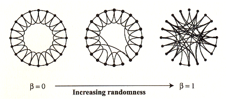
Figure 1.1: The Small World Topology.

Scale-Free Networks

While modelling systems as random graphs and the small-world models, the emphasis was modelling the network topology. The scale-free model put the emphasis on modelling network assembly and evolution. While the goal of the former models was to construct a graph with correct topological features, modelling scale-free networks put the emphasis on capturing the network dynamics reka:thesis . The Scale-Free model is composed of two constituents:

1. Growth: Starting with a small number ($m_{0}$) of nodes, at every time-step one adds a new node with $m$($\leq m_{0}$) edges that link the new node to $m$ different nodes already present in the system.

2. Preferential Attachment: When choosing the nodes to which the new node connects, one assumes that the probability $\prod$ that a new node will be connected to node $i$ depends on the degree $k_{i}$ of node $i$, such that

   $$\prod(k_{i})=\frac{k_{i}}{\sum_{j}k_{j}}.$$

Scale-free networks are characterised with power-law degree distribution.

Modularity

The concept of modularity assumes that the system’s functionality could be seamlessly partitioned into collection of modules ravsaz:science . Various networks that have been investigated so far have been found to be modular in nature, where a module is a discrete entity with several elementary components and performs an identifiable task, separable from the functions of the other modules ravsaz:science , Shen-Orr2002 .

Degree Correlations

A measure that expresses degree-degree correlation feature of the network is assortativity. It exhibits whether, in a network, nodes with poor degrees tend to connect to those with poor degrees, or, those with rich degrees. A network can be assortative, dominated by rich-to-rich node connections, or it could be disassortative with more rich-to-poor connections. A random network has no preferred degree correlation tendencies. It is known that most real-world networks (except for social networks) are disassortative r:newman and the origin of disassortativity in real-world networks is listed as “one of the ten most leading questions for network research” EPJB:round_table . This property has been shown to be having a bearing over the percolation threshold of the network r:newman .

Some of the leading questions in complex network research

Apart from origin of disassortativity, as mentioned above, many other questions are unsolved and are considered to play a potentially important role in the field of network research EPJB:round_table . Many networks in nature are found to be modular as well as hierarchical. The emergence of modularity and how it could be reconciled with other properties of networks are basic questions in network research. Networks are characterised by topology as well as the dynamics that is taking place over it. Are there universal features to the network dynamics similar to the topology? Compared to the technological networks, the evolution of biological networks is much more complex. What could be the evolutionary mechanisms that shape the topology of the biological networks? These and many other questions remain at the forefront of the network research.

Biological Networks

Among the various networks studied, biological networks are of special interest as they are the product of long evolutionary history. The mode of creation, evolution and functionality of these networks are distinct from those of technological networks.

• Biological networks are the products of natural selection as opposed to the rest of the networks.

• The time-scale at which these have evolved is orders of magnitudes larger than that of non-biological networks.

• Since each of these evolutionary machines are the outcome of ‘survival of the stable’ [book_the_selfish_gene, , page 12] rule, these systems are the most stable and robust (against all natural detrimental sources) systems known to us.

These are of academic interest for their complex, versatile, dynamic, and evolvable nature. On the practical side, understanding the nature of biological systems have direct or indirect implications to drug design, disease diagnosis and cure, epidemic control, and biotechnological applications.

Biological networks  could be characterised by the length-scale as follows.

• Ecological (Food Webs) Networks Hastings1991 , Berlow2004 , Sole2000 , Camacho2002 , Williams2002 , Dunne2002 ; (in metres)

• Inter-cellular Networks (between micrometres to millimetres)

• Protein-Protein Interaction Networks protein:yook , Mering2002 , Uetz2000 , Metabolic Pathways Networks metabolic:jeong , ravsaz:science , Almaas2004 , Almaas2005 , Gene Regulation Networks gene:reka , Farkas2003 , Shen-Orr2002 ( in micrometres)

• Macromolecular Networks–Complex Chemicals, Polymers Scala2000 (in nanometres)

Our focus is on ‘protein structures’, an interesting class of macromolecular networks. Proteins are unique among all other networks. They are constituted from a linear polymer chain of amino acids as opposed to sparsely distributed unconnected nodes as in most other networks. They evolve by changing their conformation and not by addition or removal of nodes. Their polypeptide backbone attains a stable shape through well-defined secondary structures and tertiary folds.

It is important to understand how proteins consistently fold into their native-state structures and the relevance of structure to their biological function. Network analysis of protein structures is an attempt to study the networks as complex dynamical systems composed of a web of interacting elements, and, thereof, to understand possible relevance of various network parameters.

1.4 Protein Structures as Complex Networks

Many efforts have been done to model biological systems from complex systems viewpoint Atlan2003 , Oltvai2002 , Koch1999 , Smaglik2000 , Knight2002 , Csete2002 . Specifically they have been increasingly studied as complex networks Alm2003 , Proulx2005 , Barabasi2004 , Strogatz2001 . Amongst all the biological systems, a system of special interest is that of a ‘protein’ for its structure, function, kinetics and stability. With its omnipresence in the cell and diverse functionality, it is a biomolecular system with immense implications to the cellular dynamics. It’s function is specified by the structure. The structure is also associated with it’s kinetic properties and stability. All these make a protein a very interesting system to study as a ‘complex dynamical system’. Here, we are specifically interested in studying protein structures as networks of noncovalent contacts, and the covalent backbone contacts.

1.4.1 Fine-grained vs. Coarse-grained Models

Various approaches fersht_book , baker:nature have been used for studying protein structures as well as the protein folding dynamics. Apart from other differences, these methods vary in the extent of detail with which the structure is modelled. Some consider atomic-level details Orengo1999 , Murzin1999 , whereas some reduce the structure to a chain of beads spatially constrained to a rectangular lattice with a limited number of attainable conformations mirny_shakh_PNAS_1998 . The relevance and applicability of each of these models, of course, rests on the kind of questions that are asked. While fine-grained models are heavy on resources (computer memory, time needed, complexity of coding etc.), they are better suited for questions that involve aspects of protein that, from experimental studies, are known to be dependent on fine structural details. On the other hand, coarse-grained models are of special value as they make it feasible to work with a large and complex system and offer a systems-level insight.

By virtue of a large number of constituent atoms and complexity of chemical interactions amongst them, a protein structure is a system with large degrees of freedom, rendering it immensely difficult for detailed modelling and analyses. Given the diversity in functional roles of protein and fairly large number of structural units (Number of Unique Folds, as defined by SCOP SCOP , $\approx~{}1000$ as of Oct. 2006 PDB ) that proteins are composed of, it makes sense to consider coarse-grained models as a viable option for modelling protein structures. Today, thanks to the untiring efforts of crystallographers and structural biologists across the world, and because of the advances in techniques and instruments, one has open access to a huge repository of interesting protein structures such as PDB, MSD-EBI, PDBJ, BMRB. As on $15^{th}$ August $2006$, there were a total of $38198$ structures deposited in the Protein Data Bank PDB . Also, from earlier studies Alm1999 , Riddle1997 , Kim1998 , Perl1998 , Chiti1999 , it is known that protein structures are amenable to coarse-graining while being of practical use. These facts strengthen the case of ‘coarse-grained models’ vis-à-vis detailed, fine-grained ones.

1.4.2 Range of Interactions in Proteins

Proteins are characterised by interactions happening at various ranges. Here, in the context of linear chain nature of proteins, range is defined as the distance between two interacting residues along the polypeptide. Interactions, then, can be divided into long- and short-range interactions. Apart from interactions that take place in the process of folding, many NMR experiments have shown that even after reaching the native state, proteins undergo conformational fluctuations with time scales from several nanoseconds to milliseconds. It has been suggested that such functionally important fluctuations are triggered by long-range interactions among a network of residues Dima2006 . Communication happening via such long-range interactions is central to protein function and proteins have evolved specific mechanisms to address this constraint. It has been shown that Suel2002 information about these mechanisms are embedded in the evolutionary record of a protein family. In our work, we delineate a range of interactions to study their individual importance and contribution.

1.4.3 Earlier studies on Protein Contact Networks

So far many studies have been undertaken to investigate protein structures as complex networks of interacting residues.

In an early study Crippen1978 , Crippen analysed protein structure in which effort was done to offer an objective definition of the domain of a protein. The author studied the structural organisation through a binary tree clustering algorithm for the residues of a single polypeptide chain. It was found that the protein structure is constituted of a hierarchy of segments that group together, then these clusters merge together eventually to form the complete chain.

In another similar study, Rose Rose1979 developed an automated procedure for the identification of domains in globular proteins.Through a slightly different approach Rose reached the conclusion that hierarchic organisation of structural domains is an evidence in favour of an underlying protein folding process that proceeds by hierarchic condensation.

Aszódi and Taylor cabios modelled linear polypeptides as well as 3-D proteins as non-directed graphs. They defined two topological indices, one (connectedness number) for residue-distance measure and another (effective chain length) as a foldedness measure, to compare folding topologies. They could reveal the hierarchical structure in the non-backbone connections of proteins.

Kannan and Vishveshwara kannan have used the graph spectral method to detect side-chain clusters in three-dimensional structures of proteins. The approach they described is used to detect a variety of side-chain clusters and to identify the residue which makes the largest number of interactions among the residues forming the cluster. Vishveshwara and others Brinda2005 , Brinda2005a , Brinda2006 , Krishnadev2005 , Sistla2005 have consducted many studies with amino-acid networks.

Vendruscolo et al. protnet:PRE showed that protein structures have small-world watts:book topology. They studied transition state ensemble (TSE) structures to identify the key residues that play an important role of “hubs” in the network of interactions to stabilise the structure of the transition state. They also showed that, though homopolymers have high clustering comparable to those of the proteins, their betweenness profile is uniform unlike that of the proteins.

Greene and Higman protnet:JMB studied the short-range and long-range interaction networks in protein structures and showed that long-range interaction network is not small world and its degree distribution, while having an underlying scale-free behaviour, is dominated by an exponential term indicative of a single-scale system.

Atilgan et al. protnet:Biophys studied the network properties of the core and surface of globular protein structures, and established that, regardless of size, the cores have the same local packing arrangements. They showed that connectivity distribution of residues is independent of their spatial location. They also explained, with an example of binding of two proteins, how the small-world topology could be useful in efficient and effective dissipation of energy, generated upon binding.

Aftabuddin and Kundu Aftabuddin2006 , Kundu2005 have studied protein structures as made of three classes of amino acids: hydrophobic, hydrophilic and charged. They found that average degree of the hydrophobic networks has significantly larger value than that of hydrophilic and charged networks. They also found that all amino acids’ networks and hydrophobic networks bear the signature of hierarchy; whereas the hydrophilic and charged networks do not have any hierarchical signature.

Shakhnovich and others dokholyan_pnas2002 have studied protein conformation network to study features that make a protein conformation on the folding pathway to become committed to rapidly desceding to the native state. They used a macroscopic measure of the protein contact network topology, the average graph connectivity, by constructing graphs that are based on the geometry of protein conformations. They found that average connectivity is higher for conformations with a high folding probability than for those with a high probability to unfold.

Jung et. al. jung_lee_moon studied the protein structures in search of identification of topological determinants of protein unfolding. They find that a newly introduced quantity, the impact edgre removal per residue, has a good overall correlation with protein unfolding rates.

Amitai et. al. Amitai2004 found that active site, ligand-binding and evolutionarily conserved residues, typically have high closeness, a network property, value. What separates this method from others is that this method solely depends on single protein structure’s information while making such a conclusion and does not rely on sequence conservation, comparison to other similar structures, or any prior knowledge.

In a recent paper Sol et. al. Sol2006 study proteins as systems that have a permanent flow of information between amino acids. By doing removal experiments in seven protein families they find that many of the centrally conserved residues are also important for allosteric communication. They put these results in perspective in view of network dynamics, topology, constraints on the evolution of protein structure and function.

1.5 In this thesis

The aim of this work has been to describe and study the three-dimensional native-state structures of proteins of different structural and functional classes as complex networks, enumerate the general network parameters, and study the relation of these parameters to their structural, functional, and kinetic properties at different length scales.

In our studies, we model protein structure as networks of interacting residues. We start from detailed fine-grained protein structure with atomic level details and obtain Protein Contact Network (PCN) by coarse-graining. In this process we keep positional information of $C_{\alpha}$ atoms which are representatives of the amino acids and disregard all the other information. The ‘contacts’ between any two residues represents a possible noncovalent interaction happening between them. The cut-off threshold ($R_{c}$) for deciding a contact is chosen accordingly at $8$Å. We describe the construction of PCN model in Chapter 2. We consider interactions happening at various length-scales as described in Subsection 1.4.2. Long-range Interaction Network (LIN) is a subset of PCN and comprises only of the backbone and the long-range interactions. In this chapter, we also describe the construction of LINs and different control networks. Further, we explain various visualisation schemes that we have used in our studies. Then we define and illustrate various network parameters and properties. Finally, we present the data of the proteins that will be used in our studies.

In Chapter 3 we describe our results related to small-world nature of the PCNs. We find that protein structures of diverse structural and functional classification display small-world nature. We observe that all the $80$ proteins of different classes have very high clustering coefficient. Despite being structurally different from globular proteins, even fibrous proteins are found to be having small-world signature. We find that PCNs have a clear signature of hierarchical nature on the clustering versus size profile.

PCNs are an unique class of macromolecular complex networks characterised by biological origin and evolutionary pressure. Hence one expects PCNs to show their unique nature through network properties. In Chapter 4 we find that PCNs are ‘assortative’, i.e. rich nodes tend to connect to rich nodes and poor nodes tend to make contact with each other. This is an exceptional observation as it is known that (except for social networks) all other complex networks are ‘disassortative’. We find that LINs, despite their very different degree distribution, are also assortative. This is an interesting observation as it indicates that the short-range interactions possibly don’t contribute towards the observed assortativity. In our study to investigate the role of various network features in bringing in assortativity, we show that degree distribution has a major contribution towards conferring assortativity in PCNs as well as in LINs.

In Chapter 5 we investigate biophysical correlates of the topological parameters of PCNs and LINs. For this study we use $30$ single-domain two-state folding proteins whose rate of folding is known. We find that the exceptional topological property, assortativity, has a positive correlation with the rate of folding ($ln(k_{F})$) for both PCN and LIN of the proteins. Also, we find that clustering coefficients of LINs has a very good negative correlation with the $ln(k_{F})$.

Thus with the help of our coarse-grained, complex network models we analyse protein structures and study questions relating to structure, function and kinetics.

Chapter 2 Materials and Methods

In our aim of analysing the protein structures, we developed various network models of protein structures, as well as their controls, and defined various network properties of these models. In this chapter, in Section 2.1, we describe the models that we have used and the procedure of constructing the models. Wherever required we also mention the algorithms that were used for this purpose. In Section 2.2, we describe and illustrate a few ways of visualising the network. Throughout our study we use various network parameters and properties to characterise the network system under study. In Section 2.3 we define and describe these parameters. In Section 2.4 we present the data, along with other relevant information, of the proteins that we have used in our studies. We mention the details of programming languages and the software used in Section 2.5. The pseudocodes of all the programmes (written in FORTRAN90 & MATLAB) are given in the Appendix A.

2.1 Construction of Protein Contact Networks and Controls

In our studies, we have used graph theory to model protein structures. Graphs, in general, could be used to model various kinds of systems in which nodes (vertices) represent discrete network elements and links (edges) represent a well-defined relationship between any two nodes. Below we explain two coarse-grained models of protein structure controls that were used in our studies.

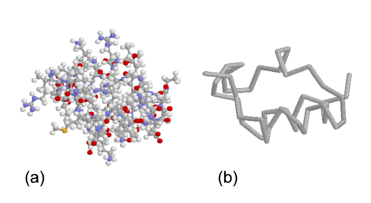
Figure 2.1: Two representations of Acyltransferase (2PDD) (a) Ball and stick representation. The colours of the atoms are attributed as specified by RasMol’s ‘CPK colour scheme’: hydrogen (white), carbon (gray), oxygen (red), nitrogen (light blue), and sulphur (yellow). (b) the backbone.

2.1.1 Protein Contact Network (PCN)

We modelled the native-state protein structure as a network made of its constituent amino-acids and their noncovalent interactions. Protein Contact Network (PCN) is a graph-theoretical representation of the protein structure, where each amino acid is a ‘node’ and spatial proximity of any two amino acids is a ‘link’ between them. Any two amino acids were considered to be in ‘spatial contact’ if the distance ($R_{c}$) between their $C_{\alpha}$ atoms was less than or equal to $8$Å. The choice of $R_{c}$ was based on the range at which non-covalent interactions, which are responsible for the polypeptide chain to fold into its native-state, are effective.

A point to note is that, apart from the noncovalent interactions, we considered the covalent peptide bonds between consecutive amino acids as links, thus representing the backbone of the protein. This chain of backbone-links was left unaltered while creating the controls, thus reflecting an important aspect of protein folding dynamics: throughout the folding process, the peptide backbone is unbroken and the protein goes through structural changes by making and breaking the noncovalent contacts.

Contact Map

Contact Map (CM) Vendruscolo1999 , Domany2000 , Banavar2001 , DEMIREL1998 , Gupta2005 , Hu2002 is a 2-D, binary, symmetric representation of the protein structure in terms of pair-wise, inter-residue contacts. Any two residues are defined to be in ‘contact’ with each other if the $C_{\alpha}$ atoms of these two residues are within a cut-off distance ($R_{c}$). Thus the contact map is a coarse-grained representation of the 3-D structure of a protein. A contact map ($\mathbf{M}$) for a protein with $n_{r}$ residues is a matrix $\mathbf{M}$ of the order $n_{r}\times n_{r}$, whose elements are defined as,

$$\mathbf{M}_{ij}=\begin{cases}1&\textit{if residues $i$ and $j$ are in contact}\\ 0&\textit{otherwise}\end{cases}$$ (2.1)

The Choice of Cut-off Distance ($R_{c}$)

The choice of cut-off distance was done based on the chemical interactions that are responsible for folding, unfolding, stability, function, etc. The chemistry of these processes is primarily dictated by chemistry of noncovalent interactions, viz., Van der Waals interactions, hydrogen bonds, ionic bonds, hydrophobic interactions. The cut-off threshold could be varied from a very high, fine-grained resolution (say, $R_{c}\approx 4$) to a very low, coarse-grained resolution. There is lower as well as upper limit to the cut-off. A value of $R_{c}$ that is less than the resolution of the protein model doesn’t make sense. And a threshold larger than the size of the protein, again, is meaningless. For our purpose, to retain the meaningful information specified by the noncovalent interactions, while at the same time not be bogged down by the atomic level details, a threshold of $R_{c}=8$Å is an ideal choice.

In our studies we have used $7$Å or $8$Å as a cut-off threshold depending on the data-set, though the results are valid for a range of thresholds between (at least) $7$–$9$Å. For practical purposes the threshold should be considered $R_{c}=8$Å throughout our studies. Various cut-offs ranging from $5$Å protnet:JMB , to $7$Å protnet:Biophys , to $8.5$Å protnet:PRE have been used in earlier studies.

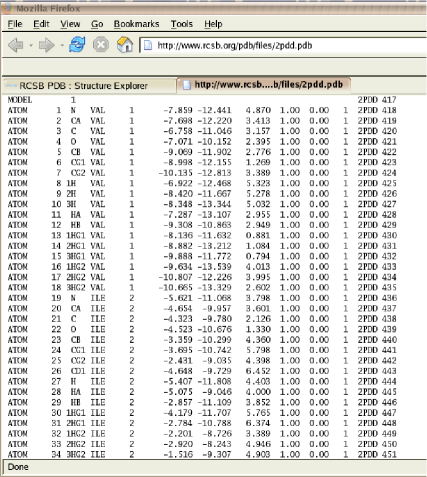
Figure 2.2: The Protein Data Bank (PDB) file containing the atomic coordinates of 2PDD (Acyltransferase).

Computational Procedure

The information required for building models of protein structures was extracted from its PDB (Protein Data Bank; http://www.rcsb.org/pdb/) file. The PDB file contains a large amount of structural details obtained from X-ray diffraction or NMR method. We explain the methodology with the example of the protein Acyltransferase (2PDD) as shown in Fig. 2.1. Figure 2.2 shows the ‘Model’ section of the PDB file in which, apart from other details, atom number, atom label, amino acid type, amino acid number, and coordinates are shown. The amino acids are labelled in increasing order from N-terminal to C-terminal residue, starting from $1$ upto $n_{r}$ ($1$ to $43$ for 2PDD), the total number of residues. First, we extracted three-dimensional coordinates of the $C_{\alpha}$ atoms (CA in Fig. 2.2), the structural representatives, of amino acids in the network models. Next, we calculated the Cartesian distances between all pairs of $C_{\alpha}$ atoms of the residues. Using a threshold $R_{c}$, (as described earlier) we computed the ‘Contact Map ($\mathbf{M}$)’. Fig. 2.3 (a) shows the pairwise distance (in $\AA$) matrix for Acyltransferase (2PDD) and (b) the corresponding Contact Map with distance threshold $R_{c}=8\AA$.

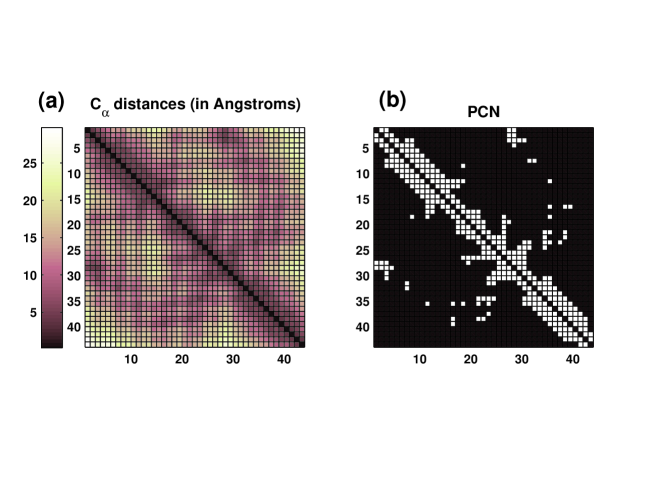
Figure 2.3: ‘Pair-wise distance matrix’ of all $C_{\alpha}$ atoms from Fig. 2.2 and Contact Map after thresholding with a cut-off of $8$Å.

The Contact Map then serves as the adjacency matrix for drawing the nodes and links of the contact network. Coarse-graining is inherent in the process of construction of PCN. Figure 2.4 summarises the process of coarse-graining involved in the making of PCN. PCN, is created by ignoring a large amount of positional information of atoms in the X-Ray data. Starting from atomic-level details (Fig. 2.4(a)), we jettison a large amount of structural details to go through residue-level details to finally arrive at the two-dimensional Contact Map (Fig. 2.4(b)). The protein contact network (PCN) can be reconstructed given the coordinates of ($C_{\alpha}$ atoms of) the residues in the structure to which the Contact Map corresponds (Fig. 2.4(c)).

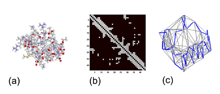
Figure 2.4: Coarse-graining of the protein structure data. (a) Ball and stick model of 2PDD, (b) its Contact Map, and (c) the PCN with $R_{c}=8$Å  where the backbone contact are shown with a blue line and the rest of the non-covalent contacts are shown in gray.

2.1.2 Long-range Interaction Network (LIN)

The Long-range Interaction Network (LIN) of a PCN was obtained by considering, other than the backbone links, only those ‘contacts’ which occur between amino acids that are ‘distant’ from each other. i.e. residue pairs that are, along the backbone, separated by a threshold, termed $LRI_{Threshold}$ of $12$ amino acids protnet:JMB or more amino acids. Here, $LRI_{Threshold}$ stands for the Long-range Interaction threshold, measured in terms of the number of residues along the backbone, that is used to decide the range upto which the ‘long-range effects’ are taking place. Thus formed, a LIN is a subset of its PCN with same number of nodes ($n_{r}$) but fewer number of links (contacts) due to removal of short-range contacts. Fig. 2.5 shows the PCN and its LIN of 2PDD.

This network is of special significance in the context of a linear chain (1-D network) model that has additional long-range links happening between nodes that are separated along the chain. A protein is one such network system in which there is an inherent 1-D structure in terms of the polypeptide backbone held together by covalent peptide bonds. The polypeptide chain folds onto itself by virtue of the chemical forces acting among the constituent residues, thereby creating ‘contacts’ on various scales as specified by the separation distance between the contacting residues.

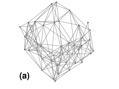
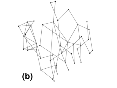
Figure 2.5: (a) PCN and (b) its LIN.

2.1.3 Random Controls of PCN

We created two types of random networks as controls for the PCNs. The polypeptide backbone connectivity was kept intact in both the random controls, while randomising the noncovalent contacts. For every protein, $100$ instances of each type of random control were generated. An average of all the instances were used as a representative of the parameters and properties that were compared with PCNs and their LINs.

Type I Random Control

The Type I random control has the same number of residues ($n_{r}$) as well as number of contacts ($n_{c}$) as those of PCN, except that the contacts are created randomly by avoiding self-contacts or duplicate contacts. The connectivity distribution of the Type I random controls, in general, is not the same as that of PCNs. The algorithmic steps used for creating the Type I random controls were as follows. We started the network with $n_{r}$ number of nodes and $n_{r}-1$ covalent contacts representing the backbone. The covalent contacts were put in place by sequentially connecting residues from $1$ to $2$ to $3$, and so on till $n_{r}$. Further, we added all the noncovalent contacts in a random manner. First we chose two unique residues using a uniform pseudo-random number generator. A noncovalent contact was created between these residues provided they were not part of the backbone-forming contacts and if they were not already connected. This process was repeated till the total number of contacts in the random control is same as those in the PCN. The ‘LINs of Type I random controls’ were obtained in the same fashion by which the LINs were obtained from PCNs. Figure 2.6 shows a typical Type-I random control (b) of 2PDD’s PCN (a) and its LIN (c).

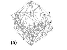
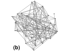
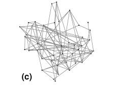
Figure 2.6: (a) PCN, (b) Type-I Random Control and (c) its LIN.

Type II Random Control

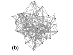
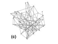
Figure 2.7: (a) PCN, (b) Type-II Random Control and (c) its LIN.

In Type II random controls, apart from maintaining the number of nodes ($n_{r}$) and contacts ($n_{c}$), the connectivity distribution as well as individual connectivity of PCNs was also conserved. We started with the original PCN and then the non-covalent contacts were randomised while maintaining the degree of individual nodes. To ensure adequate randomisation of the connectivity, the pattern of pair-connectivity was randomised $2000$ times. In Type II random controls, degree distributions of only the PCNs were conserved. For the LINs obtained from these controls of PCNs, the degree distributions were not explicitly conserved in the randomisation procedure. Figure 2.7 shows PCN (a), it’s typical Type-II random control (b), and its LIN (c).

2.2 Network Visualisation

There are various ways a graph (network) can be visualised. Depending on the purpose of the visualisation, one may want to choose appropriate visualisation method. Network systems could be classified based on the way the nodes are, if at all, positionally related to each other. A network with (a) no positional relationship among its nodes, (b) a linear relationship–a 1-D chain, (c) a 2-D order–and, finally (d) each node characterised by positional coordinates in a 3-D space.

When studying a system in which there is no structural order of the nodes, a 2-D or 3-D visualisation with arbitrary node positions optimised for minimal crossings of the links is one of the suitable choices. For a system in which a linear order is specified, a chain-like or ring-like representation would capture the necessary details. A system with 2-D (3-D) order could be represented in the 2-D (3-D) space with appropriate positions of nodes and, if necessary, with optimised edge-crossings.

Contact Map Visualisation

Contact Map has been defined and used earlier. Here we mention the visualisation aspects and its relationship to the proteins that they model. The principle diagonal of the contact map corresponds to the self-contacts which by definition are zero: $\mathbf{M}_{ii}=0.$ The positions parallel and next to the diagonal correspond to contact separation of ($|j-i|=$) $1,$ which is equivalent to the polypeptide chain that is held together with the covalent peptide bonds. The elements diagonally parallel and next to backbone represent contacts happening between residues which are one residue apart ($|j-i|=2$) along the backbone. The procedure continues so on and so forth till one reaches the single contact possible with $|j-i|=n_{r}-1$ which, when existent in a protein, indicates a contact between the N-terminal and C-terminal residue of the protein. This understanding could be used for creating appropriate models with desired types of chemical connectivities.

Chain Representation

The information content of the protein’s contact map can be transformed into a representation that offers similar insight about the range at which contacts are taking place in the protein backbone. It also gives a hint about the locations where the secondary structures are taking place. This ‘Chain Representation’ of the protein structure, though similar to that of the Contact Map, is sometimes more useful as it represents the protein structure in a less abstract and easily accessible fashion. Fig. 2.8 depicts, for Acyltransferase (2PDD), the parts that Chain Representation is composed of.

Figure 2.8 shows contact map of the network with (a) short-range contacts ($|j-i|<12$) in ‘blue’. Fig. 2.8(b) shows long-range contacts which ($|j-i|\geq 12$) are shown in ‘yellow’. Finally, Fig. 2.8(c) shows the ‘Chain Contact Map’ that is a combination of the above two. The polypeptide backbone of Acyltransferase (2PDD) is aligned as a chain of residues along a circular curve. The residues are labelled in an increasing order (anti-clockwise) from N-terminal to C-terminal. The backbone contacts, which trace the circle, are shown in black. The short-range contacts ($|j-i|<LRI_{threshold}$) are shown in blue, and those with long-range are shown in red.

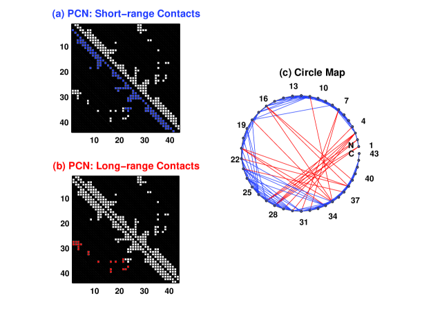
Figure 2.8: Drawing ‘Chain Contact Map’. Contact Map of PCN with (a) short-range contacts, and (b) long-range contacts highlighted.(c) ‘Circle’ or ‘Chain Contact Map’

3-D Representation

As mentioned earlier, the positional information of the residues in the protein’s 3-D structure is lost in the contact map as well as in chain representation. Owing to the relevance of the positional information, PCNs can be better visualised in 3-D space. This is achieved by superimposing ‘positional information’ with that in the ‘contact map’, as shown in Fig. 2.4 (c).

2.3 Network Parameters and Properties

Various features of network’s topology and dynamics could be measured by defining parameters that capture appropriate aspects of it. Below, we describe properties that are typically used to characterise a network. Since a network could be a directed/undirected and weighted/unweighted, the parameters need to be appropriately defined. The following definitions are valid for any undirected and unweighted network.

Here, we explain the implication of each of these parameters in the context of the network model that we build for the protein structures.

2.3.1 Distance Measures

Here, Distance is measured in terms of the number of edges that are needed to be traversed, to reach to one node from the other node. Many distance measures could then be defined which measure different aspects of the protein structure.

Characteristic Path Length

Shortest path length ($L_{ij}$), between any two pairs of nodes $i$ & $j$, is defined as the number of links that must be traversed, by the shortest route, from one node to another. The average of shortest path lengths, known as ‘characteristic path length’ ($L$), is an indicator of compactness of the network, and is defined as watts:nature ,

$$L=\frac{2~{}\sum_{i=1}^{n_{r}-1}\sum_{j=i+1}^{n_{r}}L_{ij}}{n_{r}(n_{r}-1)},$$ (2.2)

where $n_{r}$ is the number of residues in the network.

This definition is illustrated in Fig. 2.9 (a). The figure shows two of all the possible ‘paths’ between nodes $31$ and $20$ which are two of the nearest to ‘the shortest path’. Shown with blue-coloured arrows is the path $31$ $\rightarrow$ $32$ $\rightarrow$ $33$ $\rightarrow$ $34$ $\rightarrow$ $35$ $\rightarrow$ $20$, with path-length of $5$. Whereas the path with red-coloured arrows, $31$ $\rightarrow$ $7$ $\rightarrow$ $8$ $\rightarrow$ $9$ $\rightarrow$ $10$ $\rightarrow$ $11$ $\rightarrow$ $20$, has path-length of $6$. Hence the shortest path length between node $31$ and $20$ is, $L_{31,20}=5$.

Fig. 2.9 (b) shows the shortest paths distribution for the example protein network, 2PDD. Analytically, the $L$ is defined for a network with number of nodes $n_{r}$ and average degree $\langle k\rangle$ as,

$$L=\frac{n_{r}(n_{r}+\langle k\rangle-2)}{2\langle k\rangle(n_{r}-1)}$$

(a)

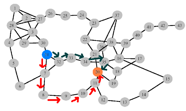
(b)

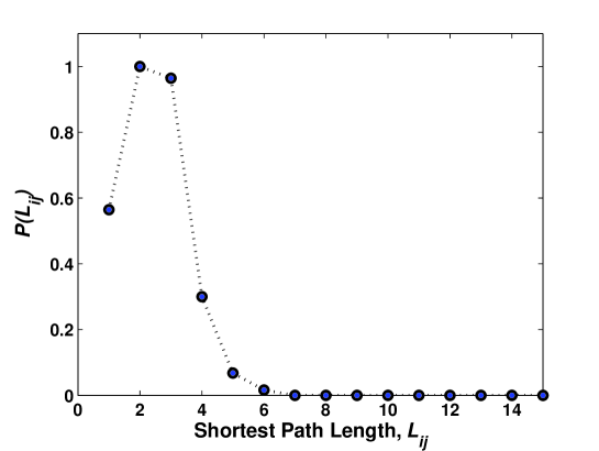
Figure 2.9: (a) Illustration of the Characteristic Path Length ($L_{ij}$), (b) Shortest Paths Distribution for 2PDD.

(a)

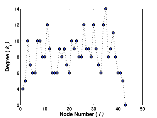
(b)

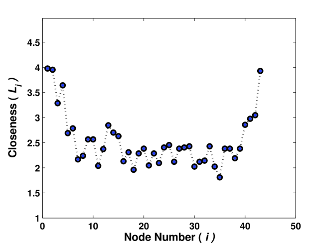
Figure 2.10: (a) Degree ($k{i}$) and (b) Closeness ($l_{i}$).

Diameter

Another measure for compactness of the network is Diameter ($D$), which is defined as the largest of all the shortest paths in the network.

$$D=\max{L_{ij}},\forall~{}\text{\emph{i--j} pairs of shortest paths.}$$ (2.3)

2.3.2 Centrality Measures

Networks representation of a complex system, by definition, embeds the complex interactions happening among the various elements of the system. Despite the distributed nature of the elements, some of them could potentially hold a ‘central’ position in the network, thereby being crucial to the topology and/or the dynamics. Centrality refers to the structural attribute of nodes in the network and not to the attribute of the node itself.

Degree and Average Degree

Degree ($k_{i}$) of a node $i$ is the total number of neighbours (linked nodes) it has.

$$k_{i}=\sum_{j=1}^{n_{r}}A_{ij}.$$ (2.4)

Thus defined, degree captures the centrality of the node in terms its connectivity. The more is the degree, the better connected it is. In PCN, degree ($k_{i}$) measures the number of other amino acids that amino acid $i$ is spatially proximal to (with given $R_{c}$) in the native state protein structure. Figure 2.10(a) shows the degrees of individual nodes of 2PDD.

It may be noted that as compared to other biological as well as technological networks, the process of formation and the constraints which shape the network structure are very different for the PCNs. Owing to the covalent backbone connections and steric and space constraints, the typical degree in PCN is much lower than that found in other networks.

Average degree, $\langle k\rangle$, of a network with $n_{r}$ nodes is defined as

$$\langle k\rangle=\frac{1}{n_{r}}{\sum_{i=1}^{n_{r}}k_{i}}.$$ (2.5)

Closeness

Closeness is defined based on the measurements of shortest path length between pairs of amino acids. It is a measure that computes the average connectivity of a residue with the rest of the network. It integrates the effect of the entire protein, measured in terms of its shortest distance from every other node, on a single residue. It is defined as,

$$L_{i}=\frac{\sum_{j=1}^{n_{r}}L_{ij}}{(n_{r}-1)}.$$ (2.6)

Figure 2.10(b) shows the closeness values of individual residues of 2PDD. Any property of an amino acid that is dependent on the average connectivity of amino acids could potentially be related to closeness. It is known that the kinetics and stability of a protein is often dependent on the chemical properties of one or a few amino acids. Given this fact the property of closeness acquires a special meaning and could possibly be used to explore functional relevance of individual amino acids.

2.3.3 ‘Pattern of Connectivity’ Measures

The parameters defined so far characterise individual nodes or pairs of nodes, measuring their distances or centrality in the network. On a level above this, the network is put in place by pattern of connectivities among nodes. This pattern could be characterised in following ways.

Degree Distribution

Degree symbolises the importance of a node from the perspective of mere connectivity—the larger the degree, the more important it is. The distribution of degrees in a network is an important feature which characterises the topology of the network. It could possibly reflect on the processes by which the network has evolved to attain the present topology. The networks in which the links between any two nodes are assigned randomly have a Poisson degree distribution bollobas1981 with most of the nodes having similar degree. Fig. 2.11(a) shows the degree distribution pattern of 2PDD.

Normalised Degree Distribution is the degree distribution normalised with the $Freq(max)$, the maximum frequency of the distribution. Henceforth $P(k)$ would denote the normalised degree distribution. $P(k)$ allows one to compare networks with disparate degree distribution profiles.

Remaining degree is simply one less than the total degree of a node r:newman . If $p_{k}$ is the distribution of the degrees, then the normalised distribution, $q_{k}$, of the remaining degree is

$$q_{k}=\frac{(k+1)p_{k+1}}{\sum_{j}jp_{j}}.$$

Coefficient of Assortativity

A network is said to show assortative mixing, or simply ‘assortative’, if the high-degree nodes in the network tend to be connected with other high-degree nodes. On the other hand, the network is said to be ‘disassortative’ if the high-degree nodes tend to be connected with other low-degree nodes. The Coefficient of Assortativity ($r$) measures the tendency of degree correlation. It is the Pearson correlation coefficient of the degrees at either end of a link and is defined r:newman as,

$$r=\frac{1}{\sigma_{q}^{2}}\sum_{jk}jk(e_{jk}-q_{j}q_{k}),$$ (2.7)

where $r$ is the coefficient of assortativity, $j$ and $k$ are the degrees of nodes, $q_{j}$ and $q_{k}$ are the remaining degree distributions, $e_{jk}$ is the joint probability distribution of the remaining degrees of the two nodes at either end of a randomly chosen link, and $\sigma_{q}^{2}$ is the variance of the distribution $q_{k}$. $r$ is a normalised degree correlation function, a global quantitative measure of degree correlations in a network, and takes values as $-1\leq r\leq 1$. The value of $r$ is zero for no specific trend in degree correlations, positive or negative for assortative or disassortative mixing, respectively.

(a)

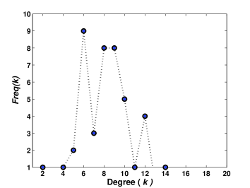
(b)

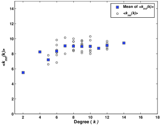
Figure 2.11: Topological Properties: (a) Degree Distribution ($P(k)$) and (b) Degree Correlations ($\langle k_{nn}(k)\rangle$)

Degree Correlations

Another way to assess the degree correlation pattern in a network is to visualise it by measuring the average degree of nearest neighbours, $k_{nn}(k)$, for nodes of degree $k$. In presence of correlation, $k_{nn}(k)$ increases with increasing $k$ for an ‘assortative network’ whereas it decreases with $k$ for a ‘disassortative network’. Fig. 2.11(b) shows the degree correlations pattern of 2PDD.

2.3.4 Compactness Measures

Clustering Coefficient

Clustering coefficient of a node $i$, $C_{i}$, is defined watts:nature as $C_{i}~{}=~{}2*n/k_{i}(k_{i}-1)$, where $n$ denotes the number of contacts amongst the $k_{i}$ neighbours of node $i$. $C_{i}$ of a node is equal to $1$ for a node whose neighbours are fully interlinked, and zero if none of the neighbouring nodes do not share any contacts. Average clustering coefficient of the network ($C$) is defined as the average of $C_{i}$s of all the nodes in the network and will be referred to as ‘clustering coefficient’ unless specified otherwise. Clustering coefficient is the measure of cliquishness of the network.

Numerically the clustering coefficient is computed as follows using the contact map.

$$C_{i}=\frac{\frac{1}{2}\sum_{j=1}^{n_{r}}\sum_{k=1}^{n_{r}}\mathbf{M}_{ij}\mathbf{M}_{ik}\mathbf{M}_{kj}}{{}^{k_{i}}C_{2}},$$ (2.8)

where, $\mathbf{M}$ is the symmetric, binary, adjacency matrix representation of the network.

Analytically, the $C$ for a network of average degree $\langle k\rangle$ is given by,

$$C=\frac{3}{4}\frac{(\langle k\rangle-2)}{(\langle k\rangle-1)}$$

Fig. 2.12 illustrates the definition of $C$. The figure shows a network with $43$ nodes of which node number $29$ and $11$ are highlighted. With the given definition of $C_{i}$, we find that $C_{29}=2/C^{3}_{2}=0.66,$ and that for node $11$ is $C_{11}=0/C^{3}_{2}=0.$ Obviously, $C$ is ‘not defined’ for isolated nodes ($k=0$), and is $0$ for nodes with degree $1$.

Figure 2.13 shows $C_{i}$’s of individual residues of 2PDD and the their histogram.

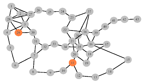
Figure 2.12: Illustration of the Clustering Coefficient ($C_{i}$).

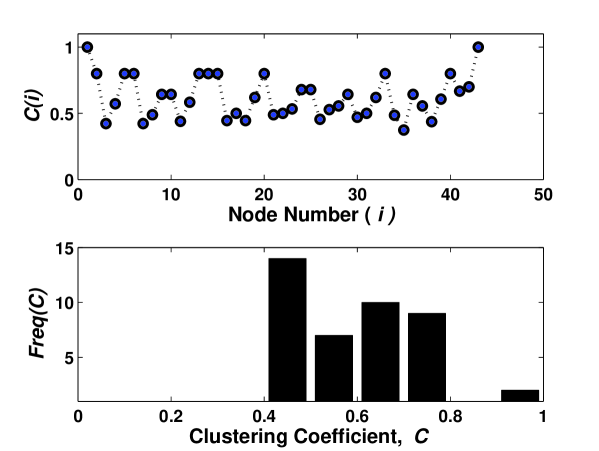
Figure 2.13: Clustering Coefficient ($C_{i}$) and its distribution ($P(C)$)

2.4 Data

For most part of the studies in (Chapter 3 and 4) we analysed a total of $80$ proteins belonging to different functional categories. Of these 80 proteins, we had 20 each from $\alpha$ (Table No. 2.1), $\beta$ (Table No. 2.2), $\alpha/\beta$ (Table No. 2.4), and $\alpha+\beta$ (Table No. 2.3) structural class. Here, we followed SCOP SCOP classification of proteins. $\alpha$ and $\beta$ class of proteins consist of proteins that are made of $\alpha$ helices and $\beta$ sheets respectively. $\alpha/\beta$ class consists of mainly parallel beta sheets ($\beta$-$\alpha$-$\beta$ units). $\alpha+\beta$ class consists of mainly anti-parallel beta sheets (segregated $\alpha$ and $\beta$ regions).

For Chapter 5 we considered only small globular proteins. These were $30$ single-domain two-state folding proteins (Table No. 2.5 and 2.6). Following tables categorise each protein in terms of name and other classification details.

PDB ID	Name	Functional Class	Size ($n_{r}$)	No. of	Resoln.
				Chains	(if X-ray)
1A6M	Oxy-Myoglobin	Oxygen Transport	151	1	1.00Å
1ALL	Allophycocynin	Light Harvesting Protein	321	2	2.30Å
1B33	Allophycocynin $\alpha$ and $\beta$ chains	Photosynthesis	2058	14	2.30Å
1C75	Cytochrome	Electron Transport	73	1	0.96Å
1DLW	Truncated Hemoglobin	Oxygen Storage/transport	116	1	1.54Å
1DO1	Carbonmonoxy-Myoglobin Mutant	Oxygen Storage/transport	153	1	1.50Å
1DWT	Myoglobin Complex	Oxygen Transport	152	1	1.40Å
1FPO	J-Type co-chperone	Chaperone	499	3	1.80Å
1FXK	Archael Prefoldin (GIMC)	Chaperone	349	3	2.30Å
1G08	Bovine Hemoglobin	Oxygen Storage/transport	572	4	1.90Å
1H97	Trematode Hemoglobin	Non-Vertebrate Hemoglobin	294	2	1.17Å
1HBR	Oxygen Storage/Transport	Chicken Hemoglobin D	570	4	2.30Å
1IDR	Oxygen Storage/Transport	Truncated Hemoglobin	253	2	1.90Å
1IRD	Oxygen Storage/Transport	Human Carbonmonoxy
		Haemoglobin	287	2	1.25Å
1KR7	Oxygen Storage/Transport	Nerve Tissue Mini-Hemoglobin	110	1	1.50Å
1KTP	Photosynthesis	C-Phycocyanin	334	2	1.60Å
1LIA	Light Harvesting Protein	R-Phycoerythrin	664	4	2.73Å
1MWC	Oxygen Storage/Transport	Wild Type Myoglobin	310	2	1.70Å
1NEK	Oxidoreductase	Succinate Dehydrogenase	1070	4	2.60Å
1PHN	Electron Transport	Phcocynin	334	2	1.65Å

Table 2.1: Data table for 20 proteins of $\alpha$ structural class.

PDB ID	Name	Functional Class	Size ($n_{r}$)	No. of	Resoln.
				Chains	(if X-ray)
1AUN	Pathogenesis-related Protein 5D	Antifungal Protein	208	1	1.80Å
1BEH	Human Phosphatidylethanemine-	Lipid Binding	367	2	1.75Å
	Binding Protein
1BHU	Streptomyces Metalloproteinase	Metalloproteinase Inhibitor	102	1	NMR
	Inhibitor
1DMH	Catechol 1	2-Dioxyoxygenase Oxidoreductase	628	2	1.70Å
1DO6	Superoxide Reductase	Oxidoreductase	248	2	2.00Å
1F35	Murine Olfactory Marker	Signaling Protein	162	1	2.30Å
1F86	Transthyretin	Transport Protein	231	2	1.10Å
1G13	Human GM2 Activator	Ligand Binding Protein	486	3	2.00Å
1HOE	$\alpha$-Amylase Inhibitor	Glycosidase Inhibitor	74	1	2.00Å
1I9R	CD40 Ligand	Cytokine/Immune System	1731	9	3.10Å
1IAZ	Equinatoxin II	Toxin	350	2	1.90Å
1IFR	Lamin–Globular Domain	Immune System	113	1	1.40Å
1JK6	Bovine NeuroPhysin	Neuropeptide	160	2	2.40Å
1KCL	Cyclodextrin glycosyl transferase	Transferase	686	1	1.94Å
1KNB	Adenovirus Type 5 Fiber Protein	Cell Receptor Recognition	186	1	1.70Å
1SFP	Acidic Seminal Fluid Protein	Spermadhesin	111	1	1.90Å
1SHS	Small Heat Shock Protein	Heat Shock Protein	920	6	2.90Å
1SLU	Rat Trypsin	Complex (serine Protease)	345	2	1.80Å
2HFT	Human Tissue Factor	Coagulation Factor	207	1	1.69Å
2MCM	Macromomycin	Apoprotein	113	1	1.50Å

Table 2.2: Data table for 20 proteins of $\beta$ structural class.

PDB ID	Name	Functional Class	Size ($n_{r}$)	No. of	Resoln.
				Chains	(if X-ray)
1AL8	Glycolate Oxidase	Flavoprotein	344	1	2.20Å
1BQC	$\beta$-Mannanase	Hydrolase	302	1	1.50Å
1BWK	Old Yellow Wnzyme Mutant	Oxidoreductase	399	1	2.30Å
1C9W	CHO Reductase	Oxidoreductase	315	1	2.40Å
1D8C	Malate Synthase G	Lyase	709	1	2.00Å
1E0W	Xylanase 10A	Glycoside Hydrolase Family 10	302	1	1.20Å
1EDG	Catalytic Domain of Celcca	Cellulose Degradation	380	1	1.60Å
1F8F	Benzyl Alcohol Dehydrogenase	Oxidoreductase	362	1	2.20Å
1FIY	Phospoenolpyruvate Carboxylase	Complex (Lysase/Inhibitor)	874	1	2.80Å
1FRB	FR-1 Protein/NADPH/	Oxidoreductase (NADP)	315	1	1.70Å
	Zopolrestat Complex
1GAD	Dehydrpgenase	Oxidoreductase	656	2	1.80Å
1HET	Liver Alcohol Dehydrogenase	Oxidoreductase	748	2	1.10Å
1HTI	Triosephosphate Isomerase (TIM)	Isomerase	496	2	2.80Å
1N8F	Mutant of Phosphate Synthase	Metal Binding Protein	1372	4	1.75Å
1OY0	Ketopantoate	Transferase	1240	5	2.80Å
	Hydroxymethyltransferase
1QO2	Ribonucleotid Isomerase	Isomerase	482	2	1.85Å
1QTW	DNA Repair Enzyme	Hydrolase	285	1	1.02Å
	Endonuclease IV
1YLV	COMPLEX	Lyase	341	1	2.15Å
2TPS	Tiamin Phosphate Synthase	Thiamin Biosynthesis	452	2	1.25Å
8RUC	Spinach Rubisco Complex	Lyase (Carbon-Carbon)	2359	8	1.50Å

Table 2.3: Data table for 20 proteins of $\alpha/\beta$ structural class.

PDB ID	Name	Functional Class	Size ($n_{r}$)	No. of	Resoln.
				Chains	(if X-ray)
1ALC	Baboon Alpha-Lactalbumin	Calcium Binding Protein	122	1	1.70Å
1AVP	Human Adenovirus 2	Hydrolase	215	2	2.60Å
	Proteinase
1BRN	Barnase	Endonuclease	216	2	1.76Å
1CNS	Chitinase	Anti-Fungal Protein	486	2	1.91Å
1CQD	Cysteine Protease	Hydrolase	864	4	2.10Å
1EUV	ULP1 Protease Domain	Hydrolase	300	2	1.60Å
1F13	Human Cellular	Coagulation Factor	1441	2	2.10Å
	Coagulation Factor XIII
1GCB	DNA-Binding Protease	DNA-Binding Protein	452	1	2.20Å
1GOU	Ribonuclease Binase	Hydrolase	218	2	1.65Å
1IWD	A Plant Cysteine	Hydrolase	215	1	1.63Å
	Protease Ervatamin
1K3B	Human Dipeptidyl	Hydrolase	352	3	2.15Å
	Peptidase I
1LNI	A Ribonuclease	Hydrolase	219	2	1.00Å
1LSD	Lysozyme	Hydrolase	129	1	1.70Å
1ME4	COMPLEX	Hydrolase	204	1	1.10Å
1MZ8	COMPLEX	Toxin Hydrolase	435	4	2.00Å
1PPN	Papain Cys-25	Hydrolase	212	1	1.60Å
1QMY	FMDV Leader Protease	Hydrolase	468	3	1.90Å
1QSA	Lytic Transglycosylase	Transferase	618	1	1.65Å
1UCH	Deubiquitinating	Cysteine Protease	206	1	1.80Å
	Enzyme UCH-L3
2ACT	Actinidin	Hydrolase (Protease)	218	1	1.70Å

Table 2.4: Data table for 20 proteins of $\alpha+\beta$ structural class.

PDB ID	$n_{r}$	Name
1HRC	104	Horse heart cytochrome C
1IMQ	86	Colicin e9 immunity protein IM9
1YCC	108	Yeast ISO-1-cytochrome C
2ABD	86	Acyl-coenzyme a binding protein from bovine liver
2PDD	43	Acetyltransferase
1APS	98	Acylphosphatase
1CIS	66	Chymotrypsin inhibitor 2 and Helix E
1COA	64	The hydrophobic core of chymotrypsin inhibitor 2
1FKB	107	Rapamycin human immunophilin FKBP-12 complex
1HDN	85	Phosphocarrier protein HPR from e. coli
1PBA	81	Activation domain of porcine procarboxypeptidase B
1UBQ	76	Ubiquitin
1URN	96	U1A mutant/RNA complex + glycerol
1VIK	99	HIV-1 protease
2HQI	72	Oxidized form of MERP
2PTL	78	Immunoglobulin light chain-binding domain of protein L
2VIK	126	Actin-severing domain villin 14T

Table 2.5: Data table for single-domain, two-state folding proteins, belonging to $\alpha$ and $\beta$ class.

PDB ID	$n_{r}$	Name
1AEY	58	Alpha-spectrin SRC homology 3 domain
1CSP	67	Bacillus subtilis major cold shock protein
1MJC	69	The major cold shock protein of e. coli
1NYF	58	SH3 domain from fyn proto-oncogene tyrosine kinase
1PKS	76	The PI3K SH3 domain
1SHF	59	The SH3 domain in Human FYN
1SHG	57	SRC-homology 3 (SH3) domain
1SRL	56	The SRC SH3 domain
1TEN	89	Fibronectin Type III domain from tenascin
1TIT	89	Titin, IG repeat 27
1WIT	93	Twitchin immunoglobulin superfamily domain
2AIT	74	Alpha-amylase inhibitor tendamistat
3MEF	69	Major cold-shock protein from escherichia coli

Table 2.6: Data table for single-domain, two-state folding proteins, belonging to $\alpha\beta$ class.

2.5 Software used

Following is the list of the software (programming languages and software utilities) used in various parts of the study.

• FORTRAN90
  Fortran90 was used to program most of the algorithms needed for the network analyses.

• MATLAB
  MatLab was primarily used for the visualisation purpose. Though extensive programming had to be done for creating intricate and detailed graphics to complement the analyses. URL: www.mathworks.com

• Gnuplot
  Since most of the work was done on Linux platform, mainly Gnuplot was used for plotting purpose. Extensive coding was done to automate the graph generation process on mass scale. URL: www.gnuplot.info

• Graphviz
  The Fortran90 code was programmed to generate standard Graphviz input file. Files so generated were fine-tuned while laying out the graphs in Graphviz. URL: www.graphviz.org

• PERL
  It was primarily used for extraction of the required data from the PDB files. URL: www.perl.com

• Octave
  Octave was used as a replacement for MatLab whenever required on the Linux platform. URL: www.octave.org

• Pajek
  This useful graph layout package was used many times, though Graphviz was preferred over Pajek. URL: vlado.fmf.uni-lj.si/pub/networks/pajek

Chapter 3 Small-World Nature of Protein Contact Networks

3.1 Introduction

There have been several efforts to study protein structures as (graphs) networks. In these studies the effort has been to analyse globular proteins as systems composed of interacting parts. In recent years, with the elaboration of network properties in a variety of real networks, Vendruscolo et al. protnet:PRE showed that protein structures have small-world topology. Greene and Higman protnet:JMB studied the short-range and long-range interaction networks in protein structures of $65$ proteins and showed that long-range interaction network is not small world and its degree distribution, while having an underlying scale-free behaviour, is dominated by an exponential term indicative of a single-scale system. Atilgan et al. protnet:Biophys studied globular protein structures and analysed the network properties of the core and surface of the proteins. They established that, regardless of size, the cores have the same local packing arrangements. They also explained, with an example of binding of two proteins, how the small-world topology could be useful in efficient and effective dissipation of energy, generated upon binding.

3.2 Small-World topology of PCNs

The small-world nature of protein networks is a basic finding. The small-world nature of a network is reflected in two properties: high clustering compared to their random controls, and a logarithmic increase in the characteristic path length with increase in the size of the network.

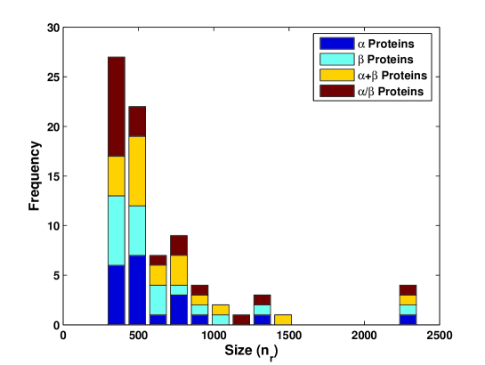
Figure 3.1: Distribution of sizes of proteins analysed.

The function that a protein serves in the cell is decided by the structure of the protein. Proteins, owing to oft-repeated structural constructs, could be classified SCOP (Structural Classification of Proteins, http://scop.mrc-lmb.cam.ac.uk/scop/) based on their structural composition. We analysed $80$ proteins (listed in Table Nos. 2.1, 2.2, 2.3, 2.4), $20$ each from four major categories ($\alpha$. $\beta$, $\alpha/\beta$, $\alpha+\beta$) of the SCOP structural classification. These are from diverse functional groups: hydrolase, transferase, protease, calcium binding, oxydoreductase, antifungal, signalling, transport, toxin, coagulation factor etc. to name a few. The size of these proteins varied from $73$ to $2359$ amino acids. Fig. 3.1 shows the histogram of size of these proteins and their break-up across the structural classes.

(a)

(b)

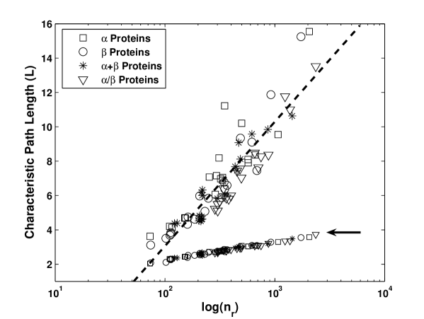
Figure 3.2: (a) $L$–$C$ plot of proteins from four structural classes. (b) Increase in the $L$ of proteins with logarithmic increase in size ($n_{r}$). The dotted line is a log-linear fit to the PCN data.

Figure 3.3: The small world nature of the proteins. Inset: Standard deviations of the corresponding data.

We calculated the average clustering coefficient ($C$) and the characteristic path length ($L$) of the proteins. Fig. 3.2 (a) shows the $L$ versus $C$ plot. As seen in the figure, on the scale of $0$ to $1$, the proteins have a very high value of clustering coefficients. Apart from very high $C$, what is interesting is that these $80$ proteins are almost indistinguishable with this parameter. Thus while presenting a generic property (that of high clustering), of proteins similar to that of a large number of other complex networks, the small-world network result provides a grim picture in terms of our ability to correlate this specific network (geometric) parameter to the proteins’ structure and function.

For a network to be classified as a small-world network, apart from high clustering, its $L$ should increase only as a $log(n_{r})$. Such a logarithmic scaling of $L$ with $n_{r}$, makes it a small-world network, i.e. any node on the network could be reached from any other node in an exceptionally few number of steps. Fig. 3.2 (b) shows that the $L$ of these $80$ PCNs scale logarithmically with the size of the network. These two properties thus ascertain the small-world nature of the PCNs across structural classes. Fig. 3.2 (b) also shows $L$ of random controls of PCNs (marked with an arrow).

Fig. 3.3 shows the summary plot of $L$–$C$ for all $80$ proteins, with their Type-I random controls in the bottom-left, regular controls in the extreme-right, and PCNs in the middle. The inset of the figure shows the means and standard deviations of $L$ and $C$ of the corresponding data. As seen in the figure the $L$ of PCNs are of the same order of magnitude as those of their Type I random controls. PCNs of these proteins have very high clustering coefficients compared to their random controls (statistically significant, $p<0.001$; Two-Sample Kolmogorov-Smirnov Test). The $L$ and $C$ computed here and in the rest of this chapter, for random and regular controls, were computed based on analytical formulae mentioned in Subsection 2.3.1 and Subsection 2.3.4 respectively.

3.3 Globular and Fibrous Proteins

Most proteins are “globular” in their three-dimensional structure, into which the polypeptide chain folds into a compact shape. In contrast, “fibrous” proteins have relatively simple, elongated three-dimensional structure suitable for their biological function (see Fig. 3.4 (b)). The “small-world” nature of globular proteins was argued protnet:Biophys to be required for enhancing the ease of dissipation of disturbances. If that were true, the fibrous proteins should depart from the small-world nature. We studied fibrous proteins and compared their network properties with globular proteins of comparable sizes. Table 3.1 shows the details of these proteins. As shown in the L–C plot in Fig. 3.4(a), fibrous proteins have larger $L$, although the $C$ are similar to those of globular proteins. Thus, in this respect, the fibrous proteins also show “small-world” properties. The average diameter for the fibrous proteins ($D=15$) was found to be larger than that of the globular proteins ($D=8.57$). This is expected because of the elongated structure of fibrous proteins. Despite this major difference in structure, the network properties of fibrous proteins and globular proteins are not very different. This indicates that the “small-world” property of proteins is generic and persists irrespective of structural differences.

Sr.No.	PDB ID	$n_{r}$	$L$	$C$
F1	1CGD	90	5.401	0.7463
F2	1CAG	88	5.274	0.6933
F3	1EI8	172	5.610	0.6045
F4	1QSU	89	5.337	0.6432
G5	1ABA	87	3.382	0.5942
G6	1AE2	86	4.066	0.5952
G6	1AYI	86	3.812	0.6025
G7	1C6R	88	3.740	0.6055
G8	1CEI	85	3.713	0.6024
G9	1CTJ	89	3.763	0.5968
G10	1DSL	88	3.404	0.5509

Table 3.1: List of four fibrous(F1–F4) and seven globular proteins(G5–G10) analysed.

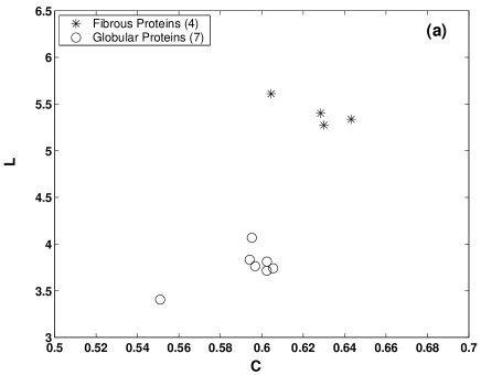
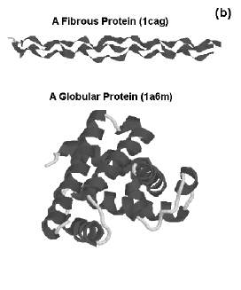
Figure 3.4: (a) L–C plot of Fibrous and Globular proteins of comparable sizes. (b) Examples of three-dimensional structures of a fibrous and globular protein (not to the scale) with their PDB codes.

3.4 $\alpha$ and $\beta$ Proteins

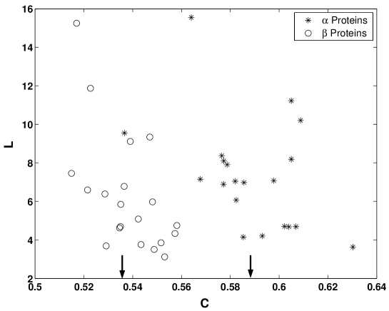
Figure 3.5: L–C plot for $\alpha$ and $\beta$ proteins. Arrows indicate the means of $C$ for $\alpha$ and $\beta$ proteins.

As seen earlier (Figure 3.2(a)), both $\alpha$ and $\beta$ class of proteins show small-world properties. Given that these are two distinct structural units one would want to know how that reflects on the global network parameters of $\alpha$ and $\beta$ proteins. On finer analysis of $L$–$C$ properties, we find that, while they are indistinguishable on $L$-scale, there is a marginal, yet consistent difference in the clustering coefficients of $\alpha$ and $\beta$ proteins as shown in Fig. 3.5. The mean of $C$ for $\alpha$ and $\beta$ proteins studied are $0.588$ and $0.538$, respectively. According to Kolmogorov-Smirnov test, this difference is statistically significant ($p<0.001$).

3.5 Degree Distributions of PCNs and LINs

The distribution of the degrees is an important property which characterises the network topology. The degree distribution of a random network is characterised by a Poisson distribution. The degree distribution of many real-world networks has been shown to be that of the scale-free type alberts . Many models have been proposed to explain the evolution of network and the degree distribution with which they are characterised at present.

We analysed the degree distribution of the $80$ proteins mentioned above. Figure 3.6 shows the normalised degree distributions of $\alpha$, $\beta$, $\alpha+\beta$, and $\alpha/\beta$ protein networks. Figure 3.6 shows the scatter plot of normalised degree distributions ($P(k)$) of all $80$ proteins of four different classes. Data points in each plot indicate $P(k)$ values for all the residues of $20$ proteins of the respective class. Solid line is a Gaussian fit to the mean of $P(k)$ for each value of $k$.

As seen, shapes of these distributions are single humped, Gaussian-like protnet:JMB . Importantly, unlike in scale-free degree distributions the number of nodes with very high degree falls off rapidly. This is interesting as in scale-free networks high-degree nodes (hubs) are known to be the facilitators of communication across the network by providing shorter routes through them. Hence hubs would partially explain small-world nature. But, clearly, the distribution of contacts in proteins is dominated by an exponential term.

Figure 3.7 shows the 1-$\sigma$ standard deviation of the data of $20$ PCNs for the normalised degree distribution of respective classes. Solid line is a Gaussian fit to $\langle P(k)\rangle$, the mean of $P(k)$ for each value of $k$. The Gaussian fit was obtained with

$$y(x)=\frac{A}{w\sqrt{\pi/2}}\exp{\frac{-2(x-x_{c})^{2}}{w^{2}}}.$$

Table 3.2 gives parameter values of the goodness of fit. Here, $R^{2}$ is the coefficient of determination.

Class	$x_{c}$	$w$	$A$	$R^{2}$
$\alpha$	$7.922$	$3.524$	$3.443$	$0.9126$
$\beta$	$8.175$	$5.429$	$6.555$	$0.9189$
$\alpha+\beta$	$7.506$	$4.216$	$5.535$	$0.9732$
$\alpha/\beta$	$7.961$	$5.192$	$6.146$	$0.9684$

Table 3.2: Degree Distribution Curve Fitting. Parameters and goodness of fit.

Degree distribution of LINs is shown in Fig. 3.8. As seen the $P(k)$ of LINs show a single-scale decay with no typical node present in them.

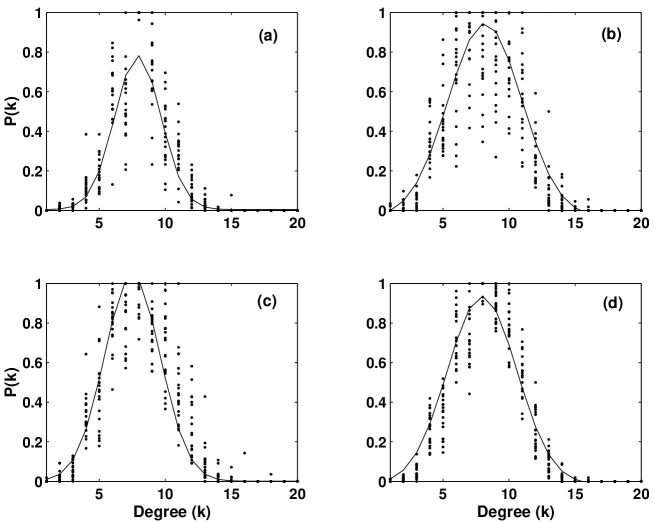
Figure 3.6: Scatter plot of degree distributions for (a) $\alpha$, (b) $\beta$, (c) $\alpha+\beta$, and (d) $\alpha/\beta$ proteins, $20$ of each class. The solid line is the Gaussian fit through the means.

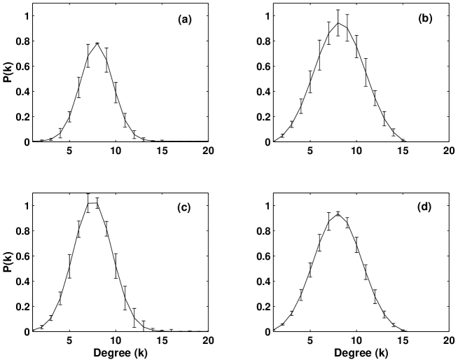
Figure 3.7: Degree distributions for (a) $\alpha$, (b) $\beta$, (c) $\alpha+\beta$, and (d) $\alpha/\beta$ proteins, $20$ of each class. The error-bars show 1-$\sigma$ standard deviation around the mean value.

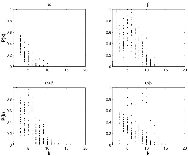
Figure 3.8: Scatter plot of degree distributions for LINs of (a) $\alpha$, (b) $\beta$, (c) $\alpha+\beta$, and (d) $\alpha/\beta$ proteins, $20$ of each class. Data points in each plot indicate $P(k)$ values for all the residues of $20$ proteins of the LINs of the PCNs of respective class.

3.6 Diameter of PCNs and LINs

The concept of diameter, strictly speaking, is applicable only to single-component graphs. Owing to the presence of the backbone connectivity, PCNs and its other versions are always single-component. Diameter is expected to scale with the number of nodes in the same way as the characteristic path length ($L$). Fig. 3.9 shows that $D$ does scale logarithmically with $n_{r}$. Diameter, since it is maximal of the distances between two nodes, the growth of $D$ with $n_{r}$ imposes upper limit on the rate of growth of $L$ with $n_{r}$.

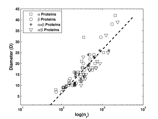
Figure 3.9: Diameter of the PCNs. (a) $\alpha$, (b) $\beta$, (c) $\alpha+\beta$, and (d) $\alpha/\beta$ proteins, $20$ of each class.

3.7 $C$–$n_{r}$ Plot

Clustering coefficient is essentially the probability of formation of triangles in the network. In a random network the probability that a given node’s two first-neighbours themselves are connected is equal to that of any two randomly selected nodes are connected. Therefore, clustering coefficient ($C_{rand}$) of a random graph is given by

$$C_{rand}=p=\frac{\langle k\rangle}{n_{r}}.$$ (3.1)

Therefore, according to Eq. 3.1 when $C_{rand}/\langle k\rangle$ of random networks is plotted as a function of $n_{r}$ for varying sizes of the network, the data will show a linear nature with slope $-1$. The random controls of PCN show such behaviour as shown in Fig. 3.10 (The data pointed with an arrow).

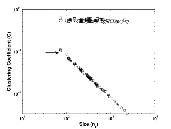
Figure 3.10: Change in $C$ of PCNs with increasing $n_{r}$, indicating the hierarchical nature of the protein structures. Random Control data is pointed with an arrow.

Figure 3.10 also shows the change in $C$ with changing size of PCNs. Here the $C$ of PCNs do not change with the size of the network ($n_{r}$) which indicates that the PCNs, far from being random, show an indication of hierarchical structure ravsaz:science in them.

3.8 Discussion

Our results show that protein networks have “small-world” property regardless of their structural classification ($\alpha$, $\beta$, $\alpha+\beta$, and $\alpha/\beta$) and tertiary structures (globular and fibrous proteins). Small world nature implies that PCNs have high degree of clustering protnet:PRE , protnet:JMB , protnet:Biophys , Bagler2005 (compared to their random counterparts). Clustering, for protein structures, represents the extent/density of packing in the network. Thus higher order compaction, observed in proteins, is in agreement with what is expected from globular polymer chains in contrast to ‘randomly folded control polymers’.

Though small but definite differences exist between $\alpha$ and $\beta$ classes, and fibrous and globular proteins. The size independence of the clustering coefficient in proteins indicates a departure from the random nature and an inherent modular organisation in the protein networks.

It is interesting to note that unlike other networks, PCNs while being small-world are not characterised by scale-free degree distribution. The absence of hubs in PCNs is understandable as there is a physical limit on the number of amino acids that can occupy the space within a certain distance around another amino acid. Such system-specific restrictions have been identified to be responsible for the emergence of different classes of networks with characteristic degree-distributions by Amaral et al. amaral:PNAS . They observed that preferential attachment to vertices in many real scale-free networks reka:thesis can be hindered by factors like ageing of the vertices (e.g. actors networks), cost of adding links to the vertices, or, the limited capacity of a vertex (e.g. airports network).

Chapter 4 Assortative Mixing in Protein Networks

4.1 Introduction

In recent years, there has been considerable interest reka:thesis , dorogovtsev:book in structure and dynamics of networks, with application to systems of diverse origins such as society (actors’ network, collaboration networks, etc.), technology (world-wide web, Internet, transportation infrastructure), biology (metabolic networks, gene regulatory networks, protein–protein interaction networks, food webs) etc. The aim of these studies has been to identify correlation between general network parameters to the structure, function, and evolution of the wide variety of systems.

Assortative Mixing

While analysing and later modelling the evolution and structure of real-world complex networks many features have been taken into account: the path length, clustering, degree distribution, and degree correlations. A lot of emphasis has been given to degree distribution. The pattern of connectivity among the nodes of varying degrees also affects the interaction dynamics of the network. Degree correlations is a measure that computes the strength and pattern of connectivity. Degree correlations were largely neglected until it was emphasised, as shown in Table 4.1, that most real-world (except social) networks are disassortative r:newman . It is evident that all real-world networks of diverse origin are characterised by disassortative mixing r:newman .

network	$n$	$r$
physics coauthorship	$52,909$	$0.363$
biology coauthorship	$1,520,251$	$0.127$
mathematics coauthorship	$253,339$	$0.120$
film actor collaborations	$449,913$	$0.208$
company directors	$7,673$	$0.276$
Internet	$10,697$	$-0.189$
World-Wide Web	$269,504$	$-0.065$
protein interactions	$2,115$	$-0.156$
neural network	$307$	$-0.163$
food web	$92$	$-0.276$

Table 4.1: Size ($n$) and assortativity coefficient ($r$) of a number of real-world networks. Data adopted from r:newman . Except for social networks, which have positive $r$s, all other networks are disassortative.

Social networks with their assortative nature, imply that they are fundamentally different from other networks and the property has been claimed newman:society01 to be originating from their unusually high clustering coefficients and community structure. Recently, assortative mixing has been demonstrated in brain functional network brainnw:eguiluz , but no biological basis has been assigned to the property. The disassortative degree mixing in most complex networks is an unsolved riddle, and questions regarding the origin of this property and whether this is an universal property of complex networks has been adjudged as “one of the ten leading questions for network research” EPJB:round_table .

Biological networks are of special interest as they are the products of long evolutionary history. The protein contact network is exclusive among other intra-cellular networks (such as metabolic networks, gene regulatory networks, protein–protein interaction networks) for their unique method of synthesis as a linear chain of amino acids, and then folding into a stable three-dimensional structure through short- and long-range contacts among the residues.

PDB ID	Class	$n_{r}$	$n_{c}$	$k_{max}$	$\langle k\rangle$	$r_{PCN}$	$r_{LIN}$
1HRC	$\alpha$	104	488	17	9.3846	0.1821	0.3531
1IMQ	$\alpha$	86	411	17	9.5581	0.2586	0.3675
1YCC	$\alpha$	108	505	17	9.3519	0.2449	0.3379
2ABD	$\alpha$	86	405	17	9.4186	0.2874	0.2736
2PDD	$\alpha$	43	175	14	8.1395	0.1436	0.2616
1AEY	$\beta$	58	271	15	9.3448	0.1145	0.2829
1CSP	$\beta$	67	308	16	9.194	0.2929	0.384
1MJC	$\beta$	69	315	16	9.1304	0.3027	0.4115
1NYF	$\beta$	58	262	15	9.0345	0.1752	0.4006
1PKS	$\beta$	76	385	17	10.1316	0.1872	0.3326
1SHF	$\beta$	59	269	16	9.1186	0.1511	0.5789
1SHG	$\beta$	57	265	16	9.2982	0.1503	0.4414
1SRL	$\beta$	56	260	16	9.2857	0.2101	0.4433
1TEN	$\beta$	89	415	17	9.3258	0.1645	0.5649
1TIT	$\beta$	89	430	17	9.6629	0.2048	0.1212
1WIT	$\beta$	93	489	17	10.5161	0.0884	0.4072
2AIT	$\beta$	74	374	17	10.1081	0.1827	0.437
3MEF	$\beta$	69	316	15	9.1594	0.3359	0.3133
1APS	$\alpha\beta$	98	489	16	9.9796	0.193	0.4822
1CIS	$\alpha\beta$	66	304	17	9.2121	0.2935	0.4823
1COA	$\alpha\beta$	64	274	17	8.5625	0.2805	0.3432
1FKB	$\alpha\beta$	107	539	15	10.0748	0.1704	0.4269
1HDN	$\alpha\beta$	85	428	16	10.0706	0.1678	0.4305
1PBA	$\alpha\beta$	81	345	14	8.5185	0.3228	0.2856
1UBQ	$\alpha\beta$	76	326	13	8.5789	0.1782	0.2977
1URN	$\alpha\beta$	96	444	18	9.25	0.3568	0.1949
1VIK	$\alpha\beta$	99	430	15	8.6869	0.5191	0.2061
2HQI	$\alpha\beta$	72	407	18	11.3056	0.145	0.1623
2PTL	$\alpha\beta$	78	334	14	8.5641	0.5179	0.3125
2VIK	$\alpha\beta$	126	616	19	9.7778	0.4144	0.464

Table 4.2: Data table for 30 single-domain two-state folding proteins of $\alpha$, $\beta$, and $\alpha\beta$ class.

Proteins are characterised by the covalent backbone connectivity. Short- as well as long-range contacts are made in the process of folding. It is known that short-range contacts are responsible for well-defined secondary structures such as $\alpha$-helix and $\beta$-sheets. The structure into which the protein chain folds and many of its properties hinge upon the long-range contacts that are made on various ‘scales’, as specified by the separation distance between the contacting residues.

Thus, PCNs are a special class of network systems. Small-world property of proteins, as studied in Chapter 3, is a reflection on the compact nature of the protein molecules. Other than that we investigated various network features of protein contact networks at different length scales (viz. PCN and LIN) in an attempt to get a better understanding of its structure, function, and stability. In this chapter we analyse assortative mixing of PCNs and LINs.

4.2 Data

In the earlier study (Chapter 3) we had considered a set of $80$ proteins, $20$ proteins each from four SCOP structural classifications. Here, we considered $30$ separate proteins to study. These $30$ proteins (Table No. 2.5 and 2.6) were single-domain, two-state folding proteins. Note: Henceforth, unless and otherwise mentioned, we use these $30$ proteins for our analyses, while supplementing it with results from other data when required. Table 4.2 gives the following details: no. of nodes, $n_{r}$, no. of contacts, $n_{c}$, maximum degree, $k_{max}$ and the average degree $\langle k\rangle$ of the PCNs, and the network parameters studied in this chapter–the coefficient of assortativity of PCNs and their LINs, $r_{PCN}$ & $r_{LIN}$.

4.3 Degree Distributions

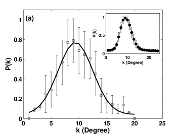
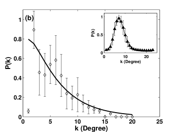
Figure 4.1: Normalised degree distributions $P(k)$ of (a) PCNs and (b) LINs. Shown in the insets are (a) Type I Random Controls of PCNs and (b) their LINs. Thick lines are the best-fit curves for the means of the data. Error-bars indicate standard deviation of the data for $P(k)$ of nodes with degree $k$ across the $30$ proteins analysed.

As done with other proteins, we first studied the normalised degree distributions of PCNs and LINs of these $30$ proteins. As seen in Fig. 4.1(a), the PCNs have Gaussian degree distribution. The parameters and expression with which the best fit was obtained are:

$$y(x)=\frac{A}{w\sqrt{\pi/2}}\exp{\frac{-2(x-x_{c})^{2}}{w^{2}}}$$

with $A=5.538$, $w=6.265$, and $x_{c}=9.373$.

On the other hand, Fig. 4.1(b) shows that the degree distribution of LINs is very different than those of PCNs. In LINs, most nodes were populated in the low-degree region and very few of them have high degrees. The best-fit for the LINs represents a single-scale exponential function protnet:JMB ,

$$P(k)\sim k^{-\gamma}\exp{(-k/k_{c})},$$

with $\gamma=0.24$ and $k_{c}=4.4$.

The nodes of degree $1$ in the degree distributions of LINs are the N- and C-terminal amino acids that are at the either end of the protein backbone. As expected bollobas1981 , the Type I random controls of the PCNs (Fig. 4.1(a), inset) have a Poisson degree distribution. LINs of Type I random controls (Fig. 4.1(b), inset) too have a Poisson degree distribution. The figure clearly shows that these properties are the same for all the proteins protnet:JMB , Bagler2005 .

4.4 Assortative nature of PCNs and LINs

We studied these $30$ single-domain, two-state folding proteins for the existence of degree-degree correlations in PCNs and LINs. We first studied $\langle k_{nn}(k)\rangle$ versus $k$ profiles of these proteins. As mentioned earlier a trend in degree correlation profile is a signature of appropriate degree mixing in the network.

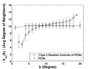
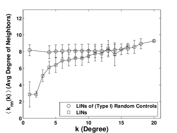
Figure 4.2: (a) Degree correlation pattern comparison between PCN and their Type-I Random Controls. (b) Comparison of degree correlation pattern of LINs and LINs of Type-I Random Controls.

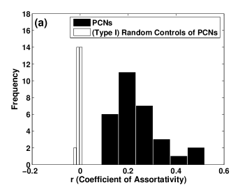
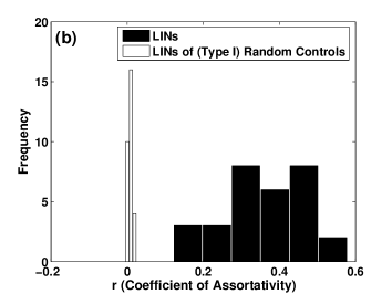
Figure 4.3: Histograms of ‘Coefficient of Assortativity ($r$)’ of (a) and (b) PCNs and LINs ($\blacksquare$) and their (Type I) Random Controls ($\square$).

Fig. 4.2 shows $\langle k_{nn}(k)\rangle$ versus $k$ plots for the PCNs ($\square$ in Fig. 4.2(a)) and LINs ($\square$ in Fig. 4.2(b)). The nature of these curves shows that both PCNs and LINs were characterised with ‘assortative mixing’, as the average degree of the neighbouring nodes increased with $k$. In comparison, the $\langle k_{nn}(k)\rangle$ remained almost constant for the Type I random control of PCNs ($\fullmoon$ in Fig. 4.2(a)) and LINs of PCNs ($\fullmoon$ in Fig. 4.2(b)), indicating lack of correlations among the nodes’ connectivity in these controls. Fig. 4.2 (a) and (b) very clearly brings forth the assortative nature of PCNs as well as their LINs.

The normalised degree correlation function, $r$, is zero for no correlations among nodes’ connectivity, and positive or negative for assortative or disassortative mixing, respectively. We computed $r_{PCN}$s and $r_{LIN}$s of the proteins (Table  4.2). The $r$ for both, PCNs and LINs of the $30$ proteins, were found to be positive, indicating that the networks are assortative. Fig. 4.3 shows the histograms of $r$ of (a) PCNs, (b) LINs, and their Type I random controls. The $r$ values of both PCNs as well as LINs of all the proteins show significantly high positive values (range: $0.09<r<0.52$ for PCNs, and $0.12<r<0.58$ for LINs). Thus these naturally-occurring, biological networks, are clearly characterised by high degree of assortative mixing. The Type I random controls in Fig. 4.3 (a & b), for both PCNs and their LINs, are distributed around zero, confirming the observation of lack of degree correlations of the controls, made in Fig. 4.2.

These properties of positive $r$ and assortative degree correlations were also observed (See Figure 4.4) for a large number of protein structures used in studies in earlier chapter belonging to diverse structural categories.

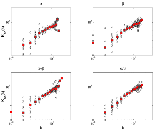
Figure 4.4: Degree correlation pattern of PCNs. Assortative mixing of PCNs. The circles ($\circ$) represent $\langle k_{nn}(k)\rangle$ for a give value of $k$ across all proteins; Filled squares averages of these values showing the trend of degree correlations.

4.5 Degree Distribution partially accounts for assortativity

To investigate the possible role of different network features we built appropriate controls as discussed in Subsec. 2.1.3. Specifically we investigated whether the distribution of degrees has any effect on observed assortativity in PCNs and LINs. We studied the ‘coefficient of assortativity’ of Type II random controls of the PCNs, in which, apart from having same number of nodes and contacts, we also preserved their degree distribution while randomising the pair-connectivities. In Fig. 4.5 and Figs. 4.6 we show that the assortativity is partially recovered in the Type II random controls for both PCNs and their LINs. Thus degree distribution partially explains the observed assortative mixing. This implies that preserving the degree distribution of PCN, even while randomising the pair-connectivities, is important in order to partially restore the assortative mixing in the random controls of PCNs as well as their LINs. The recovery of assortative mixing in the LINs by Type II random controls of PCNs is even more surprising, as the degree distribution of LINs (Fig. 4.1(b)) is very different compared to the PCNs (Fig. 4.1(a)). This is especially significant in the light of the observation brunet_2004pre , Xulvi-Brunet2005 that one can rewire the links in a (scale-free) network to obtain assortativity or disassortativity, to any degree, without any change in the degree distribution.

(a)

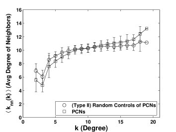
(b)

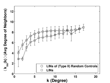
Figure 4.5: (a) Recovery of Degree correlation pattern by Type-II Random Controls of PCNs. (b) Recovery of Degree correlation pattern by LINs of Type-II Random Controls.

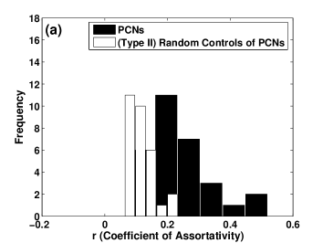
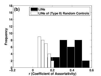
Figure 4.6: Histograms of ‘Coefficient of Assortativity ($r$)’ of (a) PCNs ($\blacksquare$) and (b) LINs ($\blacksquare$) and their (Type II) Random Controls ($\square$).

4.6 Discussion

Our coarse-grained complex network model of protein structures uncovers, for the first time in a naturally evolved biological system, the interesting, and exceptional topological feature of assortativity. The assortative nature is found to be a generic feature of protein structures.

Our discovery of assortativity in the amino acid networks in protein structures questions the invoked generality of disassortativity property in natural networks. By constructing appropriate random controls, we show (Figures. 4.5 (a, b) and Figures. 4.6(a, b)) that degree distribution can partially explain the observed assortative nature of PCNs as well their LINs. Thus, this novel feature could be a reflection on the mechanisms of contact formations in proteins while folding that have evolved through natural selection. An obvious question would be, “What are the processes by which a typical protein acquires a Gaussian-like degree distribution?”

A large number of networks are shown reka:thesis to have scale-free degree distributions. The scale-free distribution, characterised by a power law, $P(k)\sim k^{-\gamma}$, with a scaling exponent $\gamma$, is explained with the help of a growing network model with ‘preferential attachment of the nodes,’ which are being added to the network SFNW:barabasi . In addition to others’ protnet:JMB , dokholyan_pnas2002 , our results on the degree distributions (Fig. 4.1) also show that the process underlying the formation of the PCNs does not follow the ‘preferential attachment’ mode. This is understandable as the PCNs differ from other networks in many aspects. PCNs are characterised by covalent backbone connectivity which constrains the connectivity pattern. As opposed to other networks, PCNs evolve by changing the connectivity pattern through noncovalent contacts, while keeping the number of nodes constant Brinda2005 . Also in PCNs, steric hindrance limits the number of contacts an amino acid can have. All this could lead to the observed degree distribution in PCNs.

From computational studies, it has been observed r:newman , brunet_2004pre that assortative networks percolate easily, i.e., information gets easily transferred through the network as compared to that in disassortative networks. Protein folding is a cooperative phenomenon, and hence, communication amongst nodes is essential, so that appropriate noncovalent interactions can take place to form the stable native state structure foldon_englander_PNAS2005 . Thus percolation of information is very much essential and could lead to the observed cooperativity and fast folding of the proteins. Hence assortative mixing observed in proteins could be an essential prerequisite for facilitating folding of proteins.

Disassortative mixing is observed in certain networks of biological origin such as metabolic signalling pathways network, and gene regulatory network maslov:science2002 . This disassortativity is conjectured to be responsible for decreasing the likelihood of crosstalk between different functional modules of the cell, and increasing the overall robustness of a network by localising effects of deleterious perturbations. In contrast to these two networks, for the PCN one may put forward the possibility of the backbone chain connectivity as a means of conferring greater robustness against perturbations. It would also be interesting to study the role of “community structure” in conferring assortativity in these molecular networks newman:society01 , community_vicsek_nature .

Here we have shown that the assortative mixing in PCNs and LINs is a generic feature of protein structures. Also the $r$ values observed are quite high compared to other real-world networks (See Tables 4.1 and 4.2). It may be pointed out that this is the first instance of the presence of assortative mixing in a naturally occurring biological network, as all other networks studied r:newman (except for social networks) have been shown to exhibit disassortative mixing. The role, if any, the assortative nature of the protein contact networks may play in their kinetics of folding process is discussed in the next chapter.

Chapter 5 Correlation of Topological Parameters to the Rate of Folding of Two-State, Single-Domain Proteins

5.1 Introduction

In the previous chapter (Chapter 4), we showed that proteins, in general, are characterised by assortative mixing. Given that, in general, networks are known to be characterised by disassortative mixing r:newman , it brings forth an exceptional feature of proteins. It also calls for an explanation as to the purpose, if any, served by this special property. In this chapter we seek answer to this question.

In Chapter 3 we also showed that clustering coefficients($C$), which enumerate local compactness of PCNs, can not be used to distinguish proteins from each other (see the $L$–$C$ plot in Fig. 3.2). In reality, proteins are unique, function-specific and have biophysical properties which distinguish them despite structural similarities. Clearly the observed trend in characteristics path length ($L$)and clustering coefficient ($C$) are generic features that capture their compact nature and ease of communication within the structures. This indicates that either the complex network studies are limited by the coarse-grained approach to draw conclusions about the specific functionalities of protein or, that of their residues; or we need to look at different parameter(s) that capture relevant features even at this level of coarse-graining. There is evidence baker99a to suggest that coarse-graining indeed is a useful way of simplifying protein structure data while not losing the relevant biophysical details. Keeping this in view, in this chapter, we proceed to investigate both the PCNs and their long-range counterparts (LINs).

Rate of folding and Native-state topology

Though the proteins are comprised of thousands of atoms and hence potentially millions of inter-atomic interactions are possible, folding rates and mechanisms appear to be largely determined by the topology of the native (folded) state baker:nature . For network analyses and biophysical comparison we choose proteins that are structurally and kinetically simple. Hence we use single-domain, two-state folding proteins for our studies. Many geometrical parameters viz. Contact Order (CO) co , Long-range Order (LRO) lro , Total Contact Distance (TCD) tcd , that have been defined based on the native-state structure of the protein have been shown to have negatively correlated with the rate of folding ($ln(k_{F})$). Contact Order, as well as LRO and TCD which are its variants, essentially measure the average sequence separation between residues that make contacts in the 3-D structure. The correlation is remarkable given that it holds over a million-fold range of folding rates and for diverse structures. The observed negative correlation has been explained in terms of increased time needed to span the conformational space with increase in the value of these parameters. It is a reasonable explanation given that all these parameters enumerate the average normalised separation between residues those are in ‘spatial contact’ in the protein’s native-state structure.

This evidence was one of the two reasons we conjectured that our topology-based parameters may have bearing on rate of folding. The other was that our novel property of assortative mixing is independent of short-range contacts as shown in Chapter 4. Zhou and Zhou tcd reported that “the accuracy of total contact distance in predicting folding rates is essentially unchanged if ‘short’-ranged contacts ($|i-j|\leq 14$) are not included in the calculations”. Given their observation we proceeded to check if the assortativity coefficient ($r$) could have a bearing on rate of folding.

5.2 Data

The analyses was conducted with $30$ single-domain, two-state folding, globular proteins listed in Table Nos. 2.5 and 2.6. Table 5.1 provides the data for Figure 5.1. Table 5.2 provides the data for Figures 5.2, 5.3, 5.4, and 5.5. In Table 5.1 are listed the PDB IDs of the $30$ single-domain two-state folding proteins that have been used in this study and the $L$ and $C$ of their corresponding PCNs and LINs. Table 5.2 lists the coefficient of assortativity and clustering coefficients of PCNs and LINs as well as the rate of folding of these proteins.

PDB ID	Class	$L_{PCN}$	$C_{PCN}$	$L_{LIN}$	$C_{LIN}$
1HRC	$\alpha$	3.427	0.5816	5.5174	0.2713
1IMQ	$\alpha$	3.0711	0.6027	5.2774	0.1902
1YCC	$\alpha$	3.4574	0.5693	5.4283	0.2766
2ABD	$\alpha$	3.22	0.5882	4.5447	0.2289
2PDD	$\alpha$	2.4352	0.6171	4.9767	0.1612
1AEY	$\beta$	2.5529	0.6147	3.6122	0.3503
1CSP	$\beta$	2.7291	0.5954	3.8471	0.3271
1MJC	$\beta$	2.7715	0.5933	4.0273	0.3333
1NYF	$\beta$	2.5983	0.5987	3.9734	0.3457
1PKS	$\beta$	2.7421	0.5855	3.9537	0.3646
1SHF	$\beta$	2.6236	0.6059	4.2303	0.3628
1SHG	$\beta$	2.5175	0.5949	3.6028	0.3824
1SRL	$\beta$	2.5156	0.5887	3.6338	0.382
1TEN	$\beta$	3.2824	0.5738	4.3011	0.4309
1TIT	$\beta$	3.0904	0.552	4.2515	0.4519
1WIT	$\beta$	3.1346	0.5753	3.9589	0.4488
2AIT	$\beta$	2.8297	0.5922	3.726	0.4396
3MEF	$\beta$	2.7626	0.5952	3.9757	0.3136
1APS	$\alpha\beta$	3.1273	0.5676	3.9405	0.4158
1CIS	$\alpha\beta$	2.8154	0.5892	3.8424	0.349
1COA	$\alpha\beta$	2.8358	0.5768	3.9559	0.3901
1FKB	$\alpha\beta$	3.319	0.5821	4.5636	0.3626
1HDN	$\alpha\beta$	2.8538	0.5534	3.779	0.3243
1PBA	$\alpha\beta$	3.2256	0.5859	4.7802	0.2801
1UBQ	$\alpha\beta$	3.0996	0.6074	4.9846	0.3243
1URN	$\alpha\beta$	3.2529	0.5864	4.5465	0.2971
1VIK	$\alpha\beta$	3.6199	0.5849	5.2247	0.3138
2HQI	$\alpha\beta$	2.5767	0.5928	3.3521	0.3935
2PTL	$\alpha\beta$	3.972	0.599	6.982	0.2541
2VIK	$\alpha\beta$	3.4179	0.565	4.575	0.3095

Table 5.1: The PDB IDs, $L$ and $C$ values for PCN and LIN of $30$ single-domain two-state folding proteins of $\alpha$, $\beta$, and $\alpha\beta$ class of proteins.

PDB ID	Class	$r_{PCN}$	$C_{PCN}$	$r_{LIN}$	$C_{LIN}$	$ln(k_{F})$	Ref.
1HRC	$\alpha$	0.1821	0.5816	0.3531	0.2713	8.76	Chan1997
1IMQ	$\alpha$	0.2586	0.6027	0.3675	0.1902	7.31	Ferguson1999
1YCC	$\alpha$	0.2449	0.5693	0.3379	0.2766	9.62	Mines1996
2ABD	$\alpha$	0.2874	0.5882	0.2736	0.2289	6.55	Kragelund1995
2PDD	$\alpha$	0.1436	0.6171	0.2616	0.1612	9.8	Spector1999
1AEY	$\beta$	0.1145	0.6147	0.3133	0.3503	2.09	Viguera1994 , Viguera1996
1CSP	$\beta$	0.2929	0.5954	0.4822	0.3271	6.98	Perl1998
1MJC	$\beta$	0.3027	0.5933	0.4823	0.3333	5.24	lro
1NYF	$\beta$	0.1752	0.5987	0.3432	0.3457	4.54	Plaxco1998a
1PKS	$\beta$	0.1872	0.5855	0.4269	0.3646	-1.05	Guijarro1998
1SHF	$\beta$	0.1511	0.6059	0.4305	0.3628	4.55	Plaxco1998
1SHG	$\beta$	0.1503	0.5949	0.2856	0.3824	1.41	Viguera1996
1SRL	$\beta$	0.2101	0.5887	0.2977	0.382	4.04	Grantcharova1997
1TEN	$\beta$	0.1645	0.5738	0.1949	0.4309	1.06	Clarke1997
1TIT	$\beta$	0.2048	0.552	0.2061	0.4519	3.47	Fowler2001
1WIT	$\beta$	0.0884	0.5753	0.1623	0.4488	0.41	Clarke1999
2AIT	$\beta$	0.1827	0.5922	0.3125	0.4396	4.2	Schonbrunner1997
3MEF	$\beta$	0.3359	0.5952	0.464	0.3136	5.3	lro
1APS	$\alpha\beta$	0.193	0.5676	0.2829	0.4158	-1.48	Nuland1998
1CIS	$\alpha\beta$	0.2935	0.5892	0.384	0.349	3.87	lro
1COA	$\alpha\beta$	0.2805	0.5768	0.4115	0.3901	3.87	Jackson1991
1FKB	$\alpha\beta$	0.1704	0.5821	0.4006	0.3626	1.46	Main1999
1HDN	$\alpha\beta$	0.1678	0.5534	0.3326	0.3243	2.7	Nuland1998a
1PBA	$\alpha\beta$	0.3228	0.5859	0.5789	0.2801	6.8	Villegas1995
1UBQ	$\alpha\beta$	0.1782	0.6074	0.4414	0.3243	7.33	Khorasanizadeh1996
1URN	$\alpha\beta$	0.3568	0.5864	0.4433	0.2971	5.76	Silow1997
1VIK	$\alpha\beta$	0.5191	0.5849	0.5649	0.3138	6.8	Choe1998
2HQI	$\alpha\beta$	0.145	0.5928	0.1212	0.3935	0.18	tcd
2PTL	$\alpha\beta$	0.5179	0.599	0.4072	0.2541	4.1	Scalley1997
2VIK	$\alpha\beta$	0.4144	0.565	0.437	0.3095	6.8	Choe1998

Table 5.2: The $r$, $C$, of PCNs and LINs, and the corresponding rate of folding $ln(k_{F})$ for 30 single-domain two-state folding proteins. $\alpha$, $\beta$, and $\alpha\beta$ class of proteins.

5.3 Clustering Coefficients of PCNs and LINs

As shown in Chapter 3, here also we studied the $L$–$C$ properties of the $30$ proteins under consideration. To study if the PCNs of the $30$ proteins and their corresponding LINs have similar topological properties such as, characteristic path length ($L$) and clustering coefficient ($C$), we plotted the data of $L$ and $C$ from Table 5.1 in Fig. 5.1. The plot shows their corresponding Type I random controls. The Type II random controls were found to be indistinguishable from the Type I controls and not shown in Fig. 5.1.

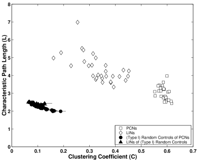
Figure 5.1: L-C plot for 30 single domain, two-state proteins: PCNs ($\square$), LINs ($\Diamond$), Type I Random Controls of PCNs ($\newmoon$) and LINs($\blacktriangle$). Error-bars in the random controls data indicate standard deviations in $L$ and $C$ for each protein computed over $100$ instances.

The results indicate two major differences between the topological properties of the PCNs and their corresponding LINs. The PCNs of these proteins have high clustering coefficients ($C>0.55$) compared to their random controls, whereas the LINs show distribution in $C$ over a range ($0.16$ to $0.45$) even though their random counterparts were almost indistinguishable from those of PCNs. $L$ and $C$ of random controls of PCNs were $2.168\pm 0.11$ & $0.1224\pm 0.0284$ and that of their LINs were $2.395\pm 0.0699$ & $0.0942\pm 0.0178$. The LINs also have marginally higher characteristic path lengths ($4.379\pm 0.7677$) than PCNs ($3\pm 0.371$) owing to their reduced number of contacts as compared to those in PCNs.

Notice that these differences in $C_{LIN}$s compared to that in $C_{PCN}$s assign specificity to the network models of proteins which is other is otherwise missing in $C_{PCN}$s.

5.4 Correlation of protein network parameters to protein folding rates

We have shown that even though the PCNs and their LINs differ in their clustering coefficients ($C$) (Fig. 5.1), both show high coefficient of assortativity ($r$) (Table 5.2) with $r_{PCN}$ being marginally lower ($0.2412\pm 0.1082$) as compared to $r_{LIN}$ ($0.36\pm 0.1102$). We now study the correlation of the network parameters to the rate of folding $ln(k_{F})$ of the corresponding proteins (Table 5.2).

5.4.1 Coefficient of Assortativity and Rate of Folding

Figure 5.2 shows the plot of $r_{PCN}$ with $ln(k_{F})$. As seen in the figure, though there is a positive trend in the data, the correlation is poor. We find that the correlation coefficient for PCNs to be $0.3776$ ($p<0.04$). The correlation becomes better ($0.5943$; $p<0.005$) after the five $\alpha$ proteins are not considered.

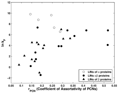
Figure 5.2: Plot of the rate of folding ($ln(k_{F})$) versus the assortativity coefficient of PCNs ($r_{PCN}s$) of $30$ proteins.

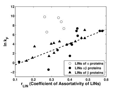
Figure 5.3: Plot of rate of folding, $ln(k_{F})$, and the Coefficient of Assortativity of LINs ($r_{LIN}$) of the PCNs of the $30$ proteins. The trend-line is shown as a dashed line.

In Fig. 5.3, the rate of folding of the 30 proteins are plotted as a function of the coefficient of assortativity of their LINs. There is an increasing trend of $\ln(k_{F})$ with increase in $r$ (correlation coefficient=$0.4221$; $p<0.02016$). Though $\beta$ and $\alpha\beta$ proteins show an increasing trend, the $5$ $\alpha$ proteins have high $ln(k_{F})$ values. The correlation coefficient between the rate of folding ($ln(k_{F})$) and $r$ of their LINs, excluding the five $\alpha$ proteins, is $0.6981$ ($p<0.0005$). This implies that, along with showing assortative mixing, the PCNs and particularly their LINs show significant positive correlations with the rate of folding. Thus the generic property of assortative mixing in proteins tend to contribute positively towards their kinetics of folding and is fairly independent of the short and long range of interactions.

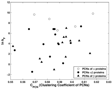
Figure 5.4: Plot of the rate of folding, $ln(k_{F})$ with Clustering Coefficient of PCNs ($C_{PCN}$).

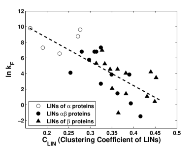
Figure 5.5: Plot of rate of folding, $ln(k_{F})$, with Clustering Coefficient of LINs ($C_{LIN}$). The trendline is indicated by a dashed line.

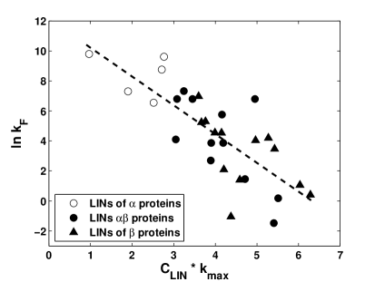
Figure 5.6: The plot of $ln(k_{F})$, with $C_{LIN}*k_{max}$.

5.4.2 Average Clustering Coefficient and Rate of Folding

Figure 5.4 shows the plot of $ln(k_{F})$ with the clustering coefficient of the PCNs ($C_{PCN}$) of the $30$ proteins. As is obvious from the plot there is hardly any correlation between the two parameters. This is borne out by the correlation coefficient that we compute as $-0.2437$ ($p<0.2$)

Figure 5.5 shows the plot of $ln(k_{F})$ with the clustering coefficient of the LINs ($C_{LIN}$). The $ln(k_{F})$ show high negative correlation (corr. coeff. $=-0.7337$; $p<0.0001$) with the $C_{LIN}$ for all the proteins.

$C_{LIN}$ enumerates number of triads made among the nodes of the Long-range Interaction Network. Thus $C_{LIN}$ essentially correlates to the number of ‘distant’ amino acids (nodes), separated by a minimum of $12$ or more other amino acids along the backbone, brought in mutual ‘contact’ with each other in the native state structure of the protein. Understandably, more the number of such long-range mutual contacts required to be made in order to achieve the native state, more is the time taken to fold, and hence slower is the rate of folding.

The calculation of clustering coefficient is dependent on the degree of the node. In Figure 5.6 we scale $C_{LIN}$s with $k_{max}$ as $C_{LIN}*k_{max}$ and plot it with $ln(k_{F})$. We find that, after scaling, the correlation coefficient improves to $-0.7712$ ($p<0.0001$). Thus $C_{LIN}$s show significantly negative correlation with single-domain, two-state folding proteins–a property completely neutralised in PCNs.

5.5 Discussion

Here we have studied two important network parameters ($C$ and $r$) of $30$ single-domain two-state folding proteins at two length-scales–PCNs and the LINs. The results show that even though the PCNs show “small-world” property in their $L$–$C$ plot, the $C_{LIN}$s have comparatively low values and are distributed over a range between the random controls and PCNs. We have studied the correlation of two widely-used topological parameters (assortativity and clustering) to the kinetics of folding at different length scales.

A ‘positive’ correlation of $ln(k_{F})$ with $r$ (Coefficient of Assortativity) is an important feature of this network as the property is maintained for both PCNs and LINs. Thus, it is a generic feature of proteins that needs fast network transmission of information for functional versatility in the cell. Apart from helping in fast folding, assortative mixing, with its role in percolation of information, could also be important for allostery and signalling in proteins that require transfer of binding information among different parts of the protein for further function. It may be noted that ‘positive’ correlation of $ln(k_{F})$ with $r$ is an exceptional feature of coefficient of assortativity as all other measures described so far co , lro , tcd have been known to have a negative correlation. Given the genetic basis and mode of formation of protein chains, the signature of assortativity as an indicator to the rate of folding is clear. It will be interesting to see which physico-chemical factors could be responsible for a positive correlation with $r$, thus speeding up the rate of folding with increasing assortative mixing of the proteins.

Most networks having high degree of clustering consist of nodes such that any two neighbours of these nodes have a high probability of themselves being linked to each other. The PCNs have been shown to have high degree of clustering, which contributes to their small-world nature helping in efficient and effective dissipation of energy needed in their function protnet:Biophys , Bagler2005 . Though the LINs have significantly lower clustering coefficients than their PCNs (Fig. 5.1) they show (Fig. 5.5) a negative correlation with the rate of folding of the proteins. This indicates that clustering of amino acids that participate in the long-range interactions, into ‘cliques’ slows down the folding process. However, the clustering coefficient of PCNs does not have any significant correlation to the rate of folding, indicating that the short-range interactions may be playing a constructive and active role in the determination of the rate of the folding process by reducing the negative contribution of the LINs. Our results clearly show that the separation of the types of contacts in the PCNs and LINs clearly delineate the length scale of contacts that play crucial role in protein folding.

Chapter 6 Conclusions

After the synthesis in the cell, folding of the amino acid chain is important for attaining the structure required to reach a functional state as soon as possible. This happens through the formation of short- as well as long-range interactions. While the former are largely responsible for formation of secondary structure units, The latter bring spatially distant (along the chain) residues closer. Secondary and tertiary structures are formed primarily by noncovalent interactions. Our graph theoretical representations of proteins structure, Proteins Contact Network (PCN) and Long-range Interaction Network (LIN), model various aspects of the three-dimensional structure of a protein in an attempt to understand it’s function and kinetics.

The Small World Nature

We found that proteins of diverse structural and functional classification have small-world nature with low characteristic path length ($L$) and high level of clustering ($C$) as shown in Figure 6.1. In this regard PCNs are similar to most other real-world networks. Interestingly, we find that LINs depart from the small-world nature. The LINs have medium range of $C$ in the proteins studied. The implication of small-world nature of PCNs is attributed to the case of dissipation of energy upon complexation. Such a property may have important role in efficient allosteric regulation of protein functions.

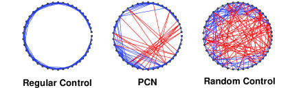
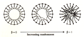
Figure 6.1: PCN and Random & Regular control of 2PDD. Comparison with Watts-Strogatz model.

Hierarchy, Modularity, and Community structure

We find that PCNs are characterised by hierarchical nature, as shown by the independence of their clustering coefficient with size (Figure 3.10). This observation is in accord with earlier findings by other researchers Rose1979 , Crippen1978 , cabios , and more investigation needs to be done on this line. We would like to point out that it has been found in many real networks ravsaz:science the hierarchy and modular architecture go hand in hand. Our preliminary results suggest modular architecture in PCNs. It would be interesting to see what significance, if any, the modules thus found in protein structures would have. Such modules could be identified by the network community structure algorithms.

Assortative Nature of PCNs and LINs

In contrast to all other naturally evolved intracellular networks studied so far, we found that contact networks of proteins show assortative mixing at both short and long length scales i.e. rich nodes tend to connect to other rich nodes. This is an exceptional property as all other real-world networks known (except for social networks) are disassortative. Interestingly, we find that LINs too are assortative, which implies that assortativity is independent of short-range interactions. We built appropriate random controls to identify the appropriate network feature that possibly contributes towards assortativity. We found that degree distribution contributes significantly towards assortative mixing in PCNs as well as their LINs.

The predominance of disassortativity in real-world networks have been alluded to confer the property of robustness (reduced spread of perturbations) in the network. Then why are the contact networks of protein structures assortative? Communication among the residues of the protein is important. It is known that “network of residues” mediate allosteric communication in proteins Suel2002 , Dima2006 . It is also proposed that allostery is an intrinsic property of all dynamic proteins Gunasekaran2004 . We propose that assortativity is an indicator of ‘allosteric communication network’ established within the protein structure and is important enough to be found in all proteins.

The role of specific residues in protein folding and their evolutionary conservation is highly debated mirny_shakh_PNAS_1998 , ScalleyKim_Baker_JMB_2004 , Larson_etal_JMB_2002 . Mirny et al. mirny_shakh_PNAS_1998 found that conserved residues that are part of folding nucleus, across proteins, were found to be in contact with each other. Based on this finding, we propose that folding nucleus of a protein could be a subset of the set of residues that form assortative group.

Our observation of assortative mixing and hence a set of residues that are part of a assortative network opens up new directions of work.

Biophysical implication of topological parameters

One would expect to have biophysical implications of the exceptional network properties that we observe. We found that for both PCNs and LINs, coefficient of assortativity, a measure of the assortativity, has positive correlation with the rate of folding of single-domain, two-state folding proteins. Similarly, we find that clustering coefficient of LINs has a high negative correlation to the rate of folding of these proteins, though that of PCNs show no significant correlation. Other workers have developed parameters specific for proteins ($CO$, $LRO$, $TCD$) and correlated with rate of folding. Our aim was to show the relevance of general network parameters to a kinetic property of the proteins. Indices such as closeness, betweenness offer more local and hence residue-specific information. By combining our general, global parameters with such local ones one could address broader questions related to protein structure and function.

Advantages and Limitations of PCN Model

PCN is, by virtue of coarse-graining, a simple model. It doesn’t involve the time evolution of the protein structure. Rather it models the static native state structure. We don’t explicitly consider information about the chemical nature of the side-chains in this model. Although, since the final native-state structure is an outcome of the chemical interactions happening among various amino acids the model implicitly does consider the chemical interactions involved.

Each of the twenty amino acids has different numbers of atoms and hence has different size. Hence the nature of noncovalent contacts depends on the specific amino acids involved. We haven’t included that information in our model so far.

The time evolution of the protein structure can be considered by building the weighted network using the Transition State Ensemble (TSE) structures. Depending on the question being asked and its sensitivity to the above-mentioned details one may consider adding further details to the PCN, thereby enhancing it.

Thus complex network analyses offers to be an important tool in studying the structure-function of proteins–the fascinating molecule of life.

Appendix A Pseudocode of the Algorithms Implemented

In this Appendix we list pseudocodes of some of the important algorithms we implemented for the complex network analyses of the proteins structures. Algorithm A lists various experiments to be performed on a single protein structure. Following is a list of frequently used variables across all the algorithms.

$n_{r}$	Number of nodes in the network
$n_{c}$	Number of links in the network
$Adj$	The $n_{r}$x$n_{r}$ Adjacency Matrix

 
Algorithm A.0.1:  ComplexNetworksAnalysis($PDBFile$)
 
$\begin{array}[]{@{\pcode@tab{1}}lr@{}}\hskip 4.30554pt\lx@intercol{}\vspace*{1ex}\mbox{comment:}\hskip 2.15277pt\mbox{The `main' function for Complex Network analyses.}\\ \hskip 4.30554pt\lx@intercol\left\{\begin{array}[]{@{}lr@{}}\mbox{{Analyse-Pcn}}(PDBFile)\\ \mbox{{Analyse-Pcn-Lin}}(Adj)\\ \mbox{{Analyse-RandomControlTypeI}}(n_{r},n_{c})\\ \mbox{{Analyse-RandomControlTypeI-LIN}}(Adj)\\ \mbox{{Analyse-RandomControlTypeII}}(Adj)\\ \mbox{{Analyse-RandomControlTypeII-LIN}}(Adj)\end{array}\right.\end{array}$
 

 
Algorithm A.0.2:  AnalysePcn($PDBFile$)
 
$\begin{array}[]{@{\pcode@tab{1}}lr@{}}\hskip 4.30554pt\lx@intercol{}\vspace*{1ex}\mbox{comment:}\hskip 2.15277pt\mbox{Function for analyses of Protein Contact Network.}\\ \hskip 4.30554pt\lx@intercol\left\{\begin{array}[]{@{}lr@{}}\mbox{{GetCoordinates}}(PDBFile)\\ \quad\mbox{return }(XYZ,n_{r})\\ \mbox{{GetAdjacencyMatrix}}(XYZ,n_{r},R_{c})\\ \quad\mbox{return }(Distances,Adj,n_{c})\\ \mbox{{GetDegree}}(Adj,n_{r})\\ \quad\mbox{return }(Degree,k_{max})\\ \mbox{{GetDegreeDistribution}}(Degree,n_{r})\\ \quad\mbox{return }(DegreeDist)\\ \mbox{{GetDegreeCorrelations}}(Degree,n_{r})\\ \quad\mbox{return }(DegreeCorrelations)\\ \end{array}\right.\end{array}$
 

 
Algorithm A.0.3:  GetAdjacencyMatrix($XYZ,n_{r},R_{c}$)
 
$\begin{array}[]{@{\pcode@tab{1}}lr@{}}\hskip 4.30554pt\lx@intercol{}\vspace*{1ex}\mbox{comment:}\hskip 2.15277pt\mbox{Function for construction of adjacency matrix.}\\ \hskip 4.30554pt\lx@intercol\mbox{procedure }\mbox{{ComputeDist}}(XYZ,i,j)\\ \hskip 4.30554pt\lx@intercol\begin{array}[]{@{\pcode@tab{1}}l@{}}\hskip 4.30554pt\lx@intercol Dist\leftarrow\sqrt{(}\sum_{k=1}^{3}(XYZ(i,k)-XYZ(j,k))^{2})\\ \hskip 4.30554pt\lx@intercol\mbox{return }(Dist)\vspace*{2ex}\end{array}\\ \hskip 4.30554pt\lx@intercol Adj\leftarrow 0\\ \hskip 4.30554pt\lx@intercol Dist\leftarrow 0\\ \hskip 4.30554pt\lx@intercol\mbox{for }i\leftarrow 1\mbox{ to }n_{r}-1\\ \hskip 4.30554pt\lx@intercol\hskip 4.30554pt\mbox{ do }\mbox{for }j\leftarrow i+1\mbox{ to }n_{r}\\ \hskip 4.30554pt\lx@intercol\hskip 4.30554pt\mbox{ do }\left\{\begin{array}[]{@{}lr@{}}Dist=\mbox{{ComputeDist}}(XYZ,i,j);\\ \mbox{if }(Dist<=R_{c}\AA)\\ \hskip 4.30554pt\mbox{ then }\left\{\begin{array}[]{@{}lr@{}}Adj(i,j)\leftarrow 1;\\ Adj(j,i)\leftarrow 1\\ Distance(i,j)\leftarrow Dist;\\ Distance(j,i)\leftarrow Dist\\ \end{array}\right.\end{array}\right.\\ \hskip 4.30554pt\lx@intercol\\ \hskip 4.30554pt\lx@intercol\mbox{return }(Adj,Dist)\end{array}$
 

 
Algorithm A.0.4:  GetDegree($Adj,n_{r}$)
 
$\begin{array}[]{@{\pcode@tab{1}}lr@{}}\hskip 4.30554pt\lx@intercol{}Degree(n_{r},2)\leftarrow 0\\ \hskip 4.30554pt\lx@intercol\mbox{for }i\leftarrow 1\mbox{ to }n_{r}\\ \hskip 4.30554pt\lx@intercol\hskip 4.30554pt\mbox{ do }\left\{\begin{array}[]{@{}lr@{}}Degree(i,1)\leftarrow 1\\ \end{array}\right.\\ \hskip 4.30554pt\lx@intercol\\ \hskip 4.30554pt\lx@intercol\mbox{for }i\leftarrow 1\mbox{ to }n_{r}\\ \hskip 4.30554pt\lx@intercol\hskip 4.30554pt\mbox{ do }\mbox{for }j\leftarrow 1\mbox{ to }n_{r}\\ \hskip 4.30554pt\lx@intercol\hskip 4.30554pt\mbox{ do }\left\{\begin{array}[]{@{}lr@{}}Degree(i,2)\leftarrow Degree(i,2)+1\\ \end{array}\right.\\ \hskip 4.30554pt\lx@intercol\\ \hskip 4.30554pt\lx@intercol DegreeMax\leftarrow\mbox{{GetDegreeMaximum}}(Degree);\\ \hskip 4.30554pt\lx@intercol\\ \hskip 4.30554pt\lx@intercol\mbox{return }(Degree,DegreeMax)\end{array}$
 

 
Algorithm A.0.5:  GetDegreeDistribution($Degree,n_{r}$)
 
$\begin{array}[]{@{\pcode@tab{1}}lr@{}}\hskip 4.30554pt\lx@intercol{}DegreeDistribution(1:n_{r},1:2)\leftarrow 0\\ \hskip 4.30554pt\lx@intercol DegreeDistributionNorm(1:n_{r},1:2)\leftarrow 0\\ \hskip 4.30554pt\lx@intercol\mbox{for }i\leftarrow 1\mbox{ to }n_{r}\\ \hskip 4.30554pt\lx@intercol\hskip 4.30554pt\mbox{ do }\left\{\begin{array}[]{@{}lr@{}}DegreeDistribution(i,1)\leftarrow i\\ DegreeDistributionNorm(i,1)\leftarrow i\\ \end{array}\right.\\ \hskip 4.30554pt\lx@intercol\\ \hskip 4.30554pt\lx@intercol\mbox{for }i\leftarrow 1\mbox{ to }n_{r}\\ \hskip 4.30554pt\lx@intercol\hskip 4.30554pt\mbox{ do }\left\{\begin{array}[]{@{}lr@{}}DegreeDistribution(Degree(i,2),2)\leftarrow\\ DegreeDistribution(Degree(i,2),2)+1\\ \end{array}\right.\\ \hskip 4.30554pt\lx@intercol\\ \hskip 4.30554pt\lx@intercol MaxDegreeDist\leftarrow\mbox{{GetMax}}(()DegreeDistribution(:,2))\\ \hskip 4.30554pt\lx@intercol DegreeDistributionNorm(:,2)\leftarrow\\ \hskip 4.30554pt\lx@intercol DegreeDistribution(:,2)/MaxDegreeDist\\ \hskip 4.30554pt\lx@intercol\\ \hskip 4.30554pt\lx@intercol\mbox{return }(DegreeDistribution,DegreeDistributionNorm)\end{array}$
 

 
Algorithm A.0.6:  GetDegreeCorrAvg($Degree,Adj,n_{r}$)
 
$\begin{array}[]{@{\pcode@tab{1}}lr@{}}\hskip 4.30554pt\lx@intercol{}DegreeCorr(1:n_{r},1:2)\leftarrow 0\\ \hskip 4.30554pt\lx@intercol DegreeCorrAvg(1:n_{r},1:2)\leftarrow 0\\ \hskip 4.30554pt\lx@intercol\mbox{for }i\leftarrow 1\mbox{ to }n_{r}\\ \hskip 4.30554pt\lx@intercol\hskip 4.30554pt\mbox{ do }\left\{\begin{array}[]{@{}lr@{}}DegreeCorr(i,1)=Degree(i,2)\\ \mbox{for }j\leftarrow 1\mbox{ to }n_{r}\\ \hskip 4.30554pt\mbox{ do }\left\{\begin{array}[]{@{}lr@{}}\mbox{if }(Adj(i,j)==1)\\ \hskip 4.30554pt\mbox{ then }\left\{\begin{array}[]{@{}lr@{}}DegreeCorr(i,2)=DegreeCorr(i,2)+Degree(j,2)\end{array}\right.\\ \end{array}\right.\end{array}\right.\\ \hskip 4.30554pt\lx@intercol\\ \hskip 4.30554pt\lx@intercol\mbox{for }i\leftarrow 1\mbox{ to }n_{r}\\ \hskip 4.30554pt\lx@intercol\hskip 4.30554pt\mbox{ do }\left\{\begin{array}[]{@{}lr@{}}DegreeCorrAvg(i,1)\leftarrow i\\ DegreeCorrAvg(DegreeCorr(i,1),2)\leftarrow\\ DegreeCorrAvg(DegreeCorr(i,1),2)+DegreeCorr(i,2)\\ \end{array}\right.\\ \hskip 4.30554pt\lx@intercol\\ \hskip 4.30554pt\lx@intercol\mbox{for }i\leftarrow 1\mbox{ to }n_{r}\\ \hskip 4.30554pt\lx@intercol\hskip 4.30554pt\mbox{ do }\left\{\begin{array}[]{@{}lr@{}}\mbox{if }(DegreeDist(i,2)/=0)\\ \hskip 4.30554pt\mbox{ then }\left\{\begin{array}[]{@{}lr@{}}DegreeCorrAvg(i,2)=DegreeCorrAvg(i,2)/DegreeDist(j,2)\end{array}\right.\\ \end{array}\right.\\ \hskip 4.30554pt\lx@intercol\\ \hskip 4.30554pt\lx@intercol\mbox{return }(DegreeCorr,DegreeCorrAvg)\end{array}$
 

 
Algorithm A.0.7:  GetCoeffAssortativity($Degree,Adj,n_{r}$)
 
$\begin{array}[]{@{\pcode@tab{1}}lr@{}}\hskip 4.30554pt\lx@intercol{}\par Term01\leftarrow 0\\ \hskip 4.30554pt\lx@intercol Term02\leftarrow 0\\ \hskip 4.30554pt\lx@intercol Term03\leftarrow 0\\ \hskip 4.30554pt\lx@intercol\mbox{for }i\leftarrow 1\mbox{ to }n_{r}\\ \hskip 4.30554pt\lx@intercol\hskip 4.30554pt\mbox{ do }\\ \hskip 4.30554pt\lx@intercol\left\{\begin{array}[]{@{}lr@{}}\mbox{for }j\leftarrow 1\mbox{ to }n_{r}\\ \hskip 4.30554pt\mbox{ do }\\ \left\{\begin{array}[]{@{}lr@{}}\mbox{if }(Adj(i,j)==1)\\ \hskip 4.30554pt\mbox{ then }\left\{\begin{array}[]{@{}lr@{}}Term01\leftarrow Term01+(Degree(i,2)*Degree(j,2))\\ Term02\leftarrow Term02+(Degree(i,2)*Degree(j,2))\\ Term03\leftarrow Term03+(Degree(i,2)^{2}+Degree(j,2)^{2})\\ \end{array}\right.\\ \end{array}\right.\end{array}\right.\\ \hskip 4.30554pt\lx@intercol\\ \hskip 4.30554pt\lx@intercol TotalEdges=\mbox{{SUM}}(()Adj)\\ \hskip 4.30554pt\lx@intercol Temp01=\frac{Term01}{TotalEdges}\\ \hskip 4.30554pt\lx@intercol Temp02={\left(\frac{Term02}{2*TotalEdges}\right)}^{2}\\ \hskip 4.30554pt\lx@intercol Temp02=\frac{Term03}{2*TotalEdges}\\ \hskip 4.30554pt\lx@intercol CoeffAssortativity=\frac{Temp01-Temp02}{Temp03-Temp02}\\ \hskip 4.30554pt\lx@intercol\\ \hskip 4.30554pt\lx@intercol\mbox{return }(CoeffAssortativity)\end{array}$
 

 
Algorithm A.0.8:  GetClusteringCoeff($Degree,Adj,n_{r}$)
 
$\begin{array}[]{@{\pcode@tab{1}}lr@{}}\hskip 4.30554pt\lx@intercol{}\par ClusteringCoeff(1:n_{r},1:2)\leftarrow 0\\ \hskip 4.30554pt\lx@intercol AvgCC\leftarrow 0\\ \hskip 4.30554pt\lx@intercol\mbox{for }i\leftarrow 1\mbox{ to }n_{r}\\ \hskip 4.30554pt\lx@intercol\hskip 4.30554pt\mbox{ do }\\ \hskip 4.30554pt\lx@intercol\left\{\begin{array}[]{@{}lr@{}}ClusteringCoeff(i,1)\leftarrow i\\ \mbox{for }i\leftarrow 1\mbox{ to }n_{r}\\ \hskip 4.30554pt\mbox{ do }\\ \left\{\begin{array}[]{@{}lr@{}}\mbox{for }j\leftarrow 1\mbox{ to }n_{r}\\ \hskip 4.30554pt\mbox{ do }\\ \left\{\begin{array}[]{@{}lr@{}}\mbox{if }(Degree(i,2)>=2)\\ \hskip 4.30554pt\mbox{ then }\left\{\begin{array}[]{@{}lr@{}}ClusteringCoeff(i,2)\leftarrow ClusteringCoeff(i,2)+\\ (Adj(i,j)*Adj(i,k)*Adj(j,k))\end{array}\right.\\ \end{array}\right.\end{array}\right.\\ \\ \mbox{if }(Degree(i,2)>=2)\\ \hskip 4.30554pt\mbox{ then }\left\{\begin{array}[]{@{}lr@{}}ClusteringCoeff(i,2)\leftarrow\frac{ClusteringCoeff(i,2)}{Degree(i,2)*(Degree(i,2)-1)}\end{array}\right.\end{array}\right.\\ \hskip 4.30554pt\lx@intercol\\ \hskip 4.30554pt\lx@intercol\mbox{for }i\leftarrow 1\mbox{ to }n_{r}\\ \hskip 4.30554pt\lx@intercol\hskip 4.30554pt\mbox{ do }\\ \hskip 4.30554pt\lx@intercol\left\{\begin{array}[]{@{}lr@{}}AvgCC=AvgCC+ClusteringCoeff(i,2)\end{array}\right.\\ \hskip 4.30554pt\lx@intercol AvgCC=AvgCC/n_{r}\\ \hskip 4.30554pt\lx@intercol\\ \hskip 4.30554pt\lx@intercol\mbox{return }(ClusteringCoeff,AvgCC)\end{array}$
 

 
Algorithm A.0.9:  GetClusteringCoeffDist($ClusteringCoeff$)
 
$\begin{array}[]{@{\pcode@tab{1}}lr@{}}\hskip 4.30554pt\lx@intercol{}ClusteringCoeffDist(1:10,1:2)\leftarrow 0\\ \hskip 4.30554pt\lx@intercol\mbox{for }i\leftarrow 1\mbox{ to }10\\ \hskip 4.30554pt\lx@intercol\hskip 4.30554pt\mbox{ do }\left\{\begin{array}[]{@{}lr@{}}ClusteringCoeffDist(i,1)=i\\ \end{array}\right.\\ \hskip 4.30554pt\lx@intercol\\ \hskip 4.30554pt\lx@intercol\mbox{for }i\leftarrow 1\mbox{ to }n_{r}\\ \hskip 4.30554pt\lx@intercol\hskip 4.30554pt\mbox{ do }\\ \hskip 4.30554pt\lx@intercol\left\{\begin{array}[]{@{}lr@{}}\mbox{if }ClusteringCoeff(i,2)>=0~{}\&~{}ClusteringCoeff(i,2)<0.1\\ ClusteringCoeffDist(1,2)=ClusteringCoeffDist(1,2)+1\\ \\ \hskip 4.30554pt\mbox{ else if }ClusteringCoeff(i,2)>=0.1~{}\&~{}ClusteringCoeff(i,2)<0.2\\ ClusteringCoeffDist(2,2)=ClusteringCoeffDist(2,2)+1\\ \\ \hskip 4.30554pt\mbox{ else if }ClusteringCoeff(i,2)>=0.2~{}\&~{}ClusteringCoeff(i,2)<0.3\\ ClusteringCoeffDist(3,2)=ClusteringCoeffDist(3,2)+1\\ \\ \hskip 4.30554pt\mbox{ else if }ClusteringCoeff(i,2)>=0.3~{}\&~{}ClusteringCoeff(i,2)<0.4\\ ClusteringCoeffDist(4,2)=ClusteringCoeffDist(4,2)+1\\ \\ \hskip 4.30554pt\mbox{ else if }ClusteringCoeff(i,2)>=0.4~{}\&~{}ClusteringCoeff(i,2)<0.5\\ ClusteringCoeffDist(5,2)=ClusteringCoeffDist(5,2)+1\\ \\ \hskip 4.30554pt\mbox{ else if }ClusteringCoeff(i,2)>=0.5~{}\&~{}ClusteringCoeff(i,2)<0.6\\ ClusteringCoeffDist(6,2)=ClusteringCoeffDist(6,2)+1\\ \\ \hskip 4.30554pt\mbox{ else if }ClusteringCoeff(i,2)>=0.6~{}\&~{}ClusteringCoeff(i,2)<0.7\\ ClusteringCoeffDist(7,2)=ClusteringCoeffDist(7,2)+1\\ \\ \hskip 4.30554pt\mbox{ else if }ClusteringCoeff(i,2)>=0.7~{}\&~{}ClusteringCoeff(i,2)<0.8\\ ClusteringCoeffDist(8,2)=ClusteringCoeffDist(8,2)+1\\ \\ \hskip 4.30554pt\mbox{ else if }ClusteringCoeff(i,2)>=0.8~{}\&~{}ClusteringCoeff(i,2)<0.9\\ ClusteringCoeffDist(9,2)=ClusteringCoeffDist(9,2)+1\\ \\ \hskip 4.30554pt\mbox{ else if }ClusteringCoeff(i,2)>=0.9~{}\&~{}ClusteringCoeff(i,2)<1.0\\ ClusteringCoeffDist(10,2)=ClusteringCoeffDist(10,2)+1\\ \end{array}\right.\\ \hskip 4.30554pt\lx@intercol\\ \hskip 4.30554pt\lx@intercol\mbox{return }(ClusteringCoeffDist)\end{array}$
 

 
Algorithm A.0.10:  GetTypeIRandomControl($n_{r},n_{c}$)
 
$\begin{array}[]{@{\pcode@tab{1}}lr@{}}\hskip 4.30554pt\lx@intercol{}adjTypeI(1:n_{r},1:n_{r})\leftarrow 0\\ \hskip 4.30554pt\lx@intercol RandomEdges=n_{c}-(n_{r}-1)\\ \hskip 4.30554pt\lx@intercol\mbox{for }i\leftarrow 1\mbox{ to }n_{r}-1\\ \hskip 4.30554pt\lx@intercol\hskip 4.30554pt\mbox{ do }\\ \hskip 4.30554pt\lx@intercol\left\{\begin{array}[]{@{}lr@{}}adjTypeI(i,i+1)\leftarrow 1\\ adjTypeI(i+1,i)\leftarrow 1\\ \end{array}\right.\\ \hskip 4.30554pt\lx@intercol\\ \hskip 4.30554pt\lx@intercol RandomEdgesCounter=0\\ \hskip 4.30554pt\lx@intercol\mbox{while }RandomEdgesCounter\leq RandomEdges\\ \hskip 4.30554pt\lx@intercol\hskip 4.30554pt\mbox{ do }\left\{\begin{array}[]{@{}lr@{}}iRan=\mbox{{RandomNumber}}(iSeed);\\ jRan=\mbox{{RandomNumber}}(jSeed);\\ i\leftarrow iRan*(n_{r}-1)+1\\ j\leftarrow jRan*(n_{r}-1)+1\\ \mbox{if }(i\neq j~{}\&\&~{}|i-j|\neq 1~{}\&\&~{}adjTypeI(i,j)\neq 1)\\ \hskip 4.30554pt\mbox{ then }\left\{\begin{array}[]{@{}lr@{}}adjTypeI(i,j)\leftarrow 1\\ adjTypeI(j,i)\leftarrow 1\\ \end{array}\right.\end{array}\right.\\ \hskip 4.30554pt\lx@intercol\mbox{return }(adjTypeI)\end{array}$
 

 
Algorithm A.0.11:  GetLin($adj,n_{r}$)
 
$\begin{array}[]{@{\pcode@tab{1}}lr@{}}\hskip 4.30554pt\lx@intercol{}\par\mbox{for }i\leftarrow 1\mbox{ to }n_{r}-1\\ \hskip 4.30554pt\lx@intercol\hskip 4.30554pt\mbox{ do }\mbox{for }j\leftarrow i+1\mbox{ to }n_{r}\\ \hskip 4.30554pt\lx@intercol\hskip 4.30554pt\mbox{ do }\left\{\begin{array}[]{@{}lr@{}}\mbox{if }(adj(i,j)==1~{}\&\&~{}j\neq i+1~{}\&\&~{}j<=i+LRIThreshold)\\ \hskip 4.30554pt\mbox{ then }\left\{\begin{array}[]{@{}lr@{}}adj(i,j)\leftarrow 0\\ adj(j,i)\leftarrow 0\\ \end{array}\right.\end{array}\right.\\ \hskip 4.30554pt\lx@intercol\\ \hskip 4.30554pt\lx@intercol\mbox{return }(adj)\end{array}$
 

 
Algorithm A.0.12:  GetTypeIIRandomControl($adj,n_{r},n_{c},EdgeRewirings$)
 
$\begin{array}[]{@{\pcode@tab{1}}lr@{}}\hskip 4.30554pt\lx@intercol{}EdgeRewiringsCounter=0\\ \hskip 4.30554pt\lx@intercol\mbox{while }EdgeRewiringsCounter<EdgeRewirings\\ \hskip 4.30554pt\lx@intercol\hskip 4.30554pt\mbox{ do }\left\{\begin{array}[]{@{}lr@{}}iRan=\mbox{{RandomNumber}}(iSeed);\\ jRan=\mbox{{RandomNumber}}(jSeed);\\ pRan=\mbox{{RandomNumber}}(pSeed);\\ qRan=\mbox{{RandomNumber}}(qSeed);\\ i\leftarrow iRan*(n_{r}-1)+1\\ j\leftarrow jRan*(n_{r}-1)+1\\ p\leftarrow pRan*(n_{r}-1)+1\\ q\leftarrow qRan*(n_{r}-1)+1\\ \\ \mbox{while }adj(i,j)==0~{}||~{}adj(p,q)==0~{}||~{}adj(i,q)==1~{}||{}\\ adj(p,j)==1~{}||~{}|i-j|<2~{}||~{}|p-q|<2~{}||~{}|i-q|<2~{}||{}\\ |p-j|<2\\ \hskip 4.30554pt\mbox{ do }\left\{\begin{array}[]{@{}lr@{}}iRan=\mbox{{RandomNumber}}(iSeed);\\ jRan=\mbox{{RandomNumber}}(jSeed);\\ pRan=\mbox{{RandomNumber}}(pSeed);\\ qRan=\mbox{{RandomNumber}}(qSeed);\\ i\leftarrow iRan*(n_{r}-1)+1\\ j\leftarrow jRan*(n_{r}-1)+1\\ p\leftarrow pRan*(n_{r}-1)+1\\ q\leftarrow qRan*(n_{r}-1)+1\\ \end{array}\right.\\ \\ adj(i,j)\leftarrow 0;adj(j,i)\leftarrow 0;\\ adj(p,q)\leftarrow 0;adj(q,p)\leftarrow 0;\\ adj(i,q)\leftarrow 1;adj(q,i)\leftarrow 1;\\ adj(p,j)\leftarrow 1;adj(j,p)\leftarrow 1;\\ \\ EdgeRewiringsCounter\leftarrow EdgeRewiringsCounter+1\end{array}\right.\\ \hskip 4.30554pt\lx@intercol\\ \hskip 4.30554pt\lx@intercol\mbox{return }(adj)\end{array}$

References

- [1] G. Taubes, “Protein Chemistry: Misfolding the way to Disease,” Science, vol. 271, pp. 1493–1495, 1996.
- [2] A. Fersht, Structure and Mechanism in Protein Science. W. H. Freeman and Company, New York, 2002.
- [3] C. Branden and J. Tooze, Introduction to Protein Structure. Garland Publishing Inc., 2 ed., 1999.
- [4] A. Aszódi and W. R. Taylor, “Connection topology of proteins,” CABIOS, vol. 9, pp. 523–529, 1993.
- [5] N. Kannan and S. Vishveshwara, “Identification of side-chain clusters in protein structures by a graph spectral method,” J. Mol. Biol., vol. 292, pp. 441–464, 1999.
- [6] M. Vendruscolo, N. V. Dokholyan, E. Paci, and M. Karplus, “Small-world view of the amino acids that play a key role in protein folding,” Phys. Rev. E, vol. 65, p. 061910, 2002.
- [7] L. H. Greene and V. A. Higman, “Uncovering network systems within protein structures,” J. Mol. Biol., vol. 334, pp. 781–791, 2003.
- [8] A. R. Atilgan, P. Akan, and C. Baysal, “Small-world communication of residues and significance for protein dynamics,” Biophysical J., vol. 86, pp. 85–91, 2004.
- [9] G. Bagler and S. Sinha, “Network properties of protein structures,” Physica A, vol. 346, no. 1-2, pp. 27–33, 2005.
- [10] K. V. Brinda and S. Vishveshwara, “A network representation of protein structures: implication to protein stability,” Biophysical J., vol. 89, no. 6, pp. 4159–70, 2005.
- [11] G. Amitai, A. Shemesh, E. Sitbon, M. Shklar, D. Netanely, I. Venger, and S. Pietrokovski, “Network analysis of protein structures identifies functional residues,” J. Mol. Biol., vol. 344, pp. 1135–1146, 2004.
- [12] C. Levinthal, “How to fold graciously,” in Mossbauer Spectroscopy in Biological Systems: Proceedings of a meeting held at Allerton House, Monticello, Illinois (J. T. P. DrBrunner and E. Munck, eds.), pp. 22–24, University of Illunois Press, 1969.
- [13] C. B. Anfinsen, “Principles that govern the folding of protein chains,” Science, vol. 181, pp. 223–230, 1973.
- [14] D. Bray, “Protein molecules as computational elements in living cells,” Nature, vol. 376, no. 6538, pp. 307–312, 1995.
- [15] B. Bollobás, Random Graphs. Cambridge University Press, 2001.
- [16] R. Albert and A.-L. Barabási, “Statistical mechanics of complex networks,” Rev. Mod. Phys., vol. 74, pp. 47–97, 2002.
- [17] S. H. Yook, H. Jeong, and A.-L. Barabási, “Modeling the Internet’s large-scale topology,” Proc. Natl. Acad. Sci. (USA), vol. 99, pp. 13382–13386, 2002.
- [18] R. Pastor-Satorras, A. Vázquez, and A. Vespignani, “Dynamical and correlation properties of Internet,” Phys. Rev. Lett., vol. 87, p. 258701, 2001.
- [19] M. Faloutsos, P. Faloutsos, and C. Faloutsos, “On power-law relationships of the Internet topology,” Comp. Comm. Rev., vol. 29, pp. 251–262, 1999.
- [20] R. Albert, H. Jeong, and A.-L. Barabási, “The diameter of the World Wide Web,” Nature, vol. 401, pp. 130–131, 1999.
- [21] L. A. Adamic and B. A. Huberman, “Power-law distribution of the World Wide Web,” Science, vol. 287, p. 2115a, 2000.
- [22] A.-L. Barabási, R. Albert, and H. Jeong, “Scale-free characteristics of random networks: The topology of the World Wide Web,” Physica A, vol. 281, pp. 69–77, 2000.
- [23] P. Sen, S. Dasgupta, A. Chatterjee, P. A. Sreeram, G. Mukherjee, and S. S. Manna, “Small-world properties of the Indian Railway network,” Phys. Rev. E, vol. 67, p. 36106, 2003.
- [24] A. Barrat, M. Barthélemy, R. Pastor-Satorras, and A. Vespignani, “The architecture of complex weighted networks,” Proc. Natl. Acad. Sci. (USA), vol. 101, pp. 3747–3752, 2004.
- [25] G. Bagler, “Analysis of the Airport Network of India as a complex weighted network,” arXiv:cond-mat/0409773, 2004.
- [26] M. E. J. Newman, “Why social networks are different from other type of networks,” Phys. Rev. E, vol. 68, p. 036122, 2003.
- [27] M. E. J. Newman, “The structure of scientific collaboration networks,” Proc. Natl. Acad. Sci. (USA), vol. 98, pp. 404–409, 2001.
- [28] M. E. J. Newman, “Assortative mixing in networks,” Phys. Rev. Lett., vol. 89, p. 208701, 2002.
- [29] S. N. Dorogovtsev and J. F. F. Mendes, “Evolution of networks,” Advances in Physics, vol. 51, pp. 1079–1187, 2002.
- [30] D. J. Watts and S. H. Strogatz, “Collective dynamics of ‘small-world’ networks,” Nature, vol. 393, pp. 440–442, 1999.
- [31] D. J. Watts, Small Worlds – The Dynamics of Networks Between Order and Randomness. Princeton University Press, 1999.
- [32] E. Ravsaz, A. L. Somera, D. A. Mongru, Z. N. Oltvai, and A.-L. Barabási, “Hierarchical organization of modularity in metabolic networks,” Science, vol. 297, pp. 1551–1555, 2002.
- [33] S. S. Shen-Orr, R. Milo, S. Mangan, and U. Alon, “Network motifs in the transcriptional regulation network of Escherichia coli,” Nat. Genet., vol. 31, no. 1, pp. 64–68, 2002.
- [34] L. A. N. Amaral, A. Barrat, A. L. Barabasi, G. Caldarelli, P. D. L. Rios, A. Erzan, B. Kahng, R. Mantegna, J. F. F. Mendes, R. Pastor-Satorras, and A. Vespignani, “Virtual round table on ten leading questions for network research,” Eur. Phys. J. B, vol. 38, pp. 143–145, 2004.
- [35] R. Dawkins, The Selfish Gene (Indian Edition). Oxford University Press, first ed., 2005.
- [36] A. Hastings and T. Powell, “Chaos in a 3-species food-chain,” Ecology, vol. 72, pp. 896––903, 1991.
- [37] E. L. Berlow, A.-M. Neutel, J. E. Cohen, P. C. de Ruiter, B. Ebenman, M. Emmerson, J. W. Fox, V. A. A. Jansen, J. I. Jones, G. D. Kokkoris, D. O. Logofet, A. J. McKane, J. M. Montoya, and O. Petchey, “Interaction strengths in food webs: issues and opportunities,” Journal of Animal Ecology, vol. 73, no. 3, pp. 585–598, 2004.
- [38] J. M. Montoya and R. V. Sole, “Small world patterns in food webs,” J. Theor. Biol., vol. 214, no. 3, 2000.
- [39] J. Camacho, R. Guimerà, and L. A. N. Amaral, “Robust patterns in food web structure,” Phys. Rev. Lett., vol. 88, p. 228102, 2002.
- [40] R. J. Williams, E. L. Berlow, J. A. Dunne, A.-L. Barabasi, and N. D. Martinez, “Two degrees of separation in complex food webs,” Proc. Natl. Acad. Sci. (USA), vol. 99, no. 20, pp. 12913–12916, 2002.
- [41] J. A. Dunne, R. J. Williams, and N. D. Martinez, “Food-web structure and network theory: The role of connectance and size,” Proc. Natl. Acad. Sci. (USA), vol. 99, no. 20, pp. 12917–12922, 2002.
- [42] S. Y. Yook, Z. N. Oltvai, and A.-L. Barabási, “Functional and topological characterization of protein interaction networks,” Proteomics, vol. 4, pp. 928–942, 2004.
- [43] C. von Mering, R. Krause, B. Snel, M. Cornell, S. G. Oliver, S. Fields, and P. Bork, “Comparative assessment of large-scale data sets of protein–protein interactions,” Nature, vol. 417, no. 6887, pp. 399–403, 2002.
- [44] P. Uetz, L. Giot, G. Cagney, T. A. Mansfield, R. S. Judson, J. R. Knight, D. Lockshon, V. Narayan, M. Srinivasan, P. Pochart, A. Qureshi-Emili, Y. Li, B. Godwin, D. Conover, T. Kalbfleisch, G. Vijayadamodar, M. Yang, M. Johnston, S. Fields, and J. M. Rothberg, “A comprehensive analysis of protein–-protein interactions in saccharomyces cerevisiae,” Nature, vol. 403, no. 6770, pp. 623–627, 2000.
- [45] H. Jeong, B. Tombor, R. Albert, Z. N. Oltvai, and A.-L. Barabási, “The large-scale organization of metabolic networks,” Nature, vol. 407, pp. 651–654, 2000.
- [46] E. Almaas, B. Kovacs, T. Vicsek, Z. Oltvai, and A.-L. Barabási, “Global organization of metabolic fluxes in the bacterium Escherichia coli,” Nature, vol. 427, pp. 839–843, 2004.
- [47] E. Almaas, Z. N. Oltvai, and A.-L. Barabási, “The activity reaction core and plasticity of metabolic networks,” PLoS Computational Biology, vol. 1, pp. 0557–0563, 2005.
- [48] R. Albert and H. G. Othmer, “The topology of the regulatory interactions predicts the expression pattern of the drosophila segment polarity genes,” J. Theor. Biol., vol. 223, pp. 1–18, 2003.
- [49] I. Farkas, H. Jeong, T. Vicsek, A.-L. Barabási, and Z. Oltvai, “The topology of transcription regulatory network in the yeast, Saccharomyces cerevisiae,” Physica A, vol. 318, pp. 601–612, 2003.
- [50] A. Scala, L. Amaral, and M. Barthelemy, “Small-world networks and the conformation space of a lattice polymer chain,” www.arxiv.org/cond-mat/0004380, 2000.
- [51] H. Atlan, “The living cell as a paradigm for complex natural systems,” ComPlexUs, vol. 1, pp. 1–3, 2003.
- [52] Z. Oltvai and A. Barabási, “Life’s complexity pyramid,” Science, vol. 298, pp. 763–764, 2002.
- [53] C. Koch and G. Laurent, “Complexity and the nervous system,” Science, vol. 284, no. 5411, pp. 96–98, 1999.
- [54] P. Smaglik, “For my next trick. . .,” Nature, vol. 407, no. 6806, pp. 828–829, 2000.
- [55] J. Knight, “Physics meets biology: Bridging the culture gap,” Nature, vol. 419, no. 6904, pp. 244–246, 2002.
- [56] M. Csete and J. Doyle, “Reverse engineering of biological complexity,” Science, vol. 295, no. 5560, pp. 1664–1669, 2002.
- [57] E. Alm and A. P. Arkin, “Biological networks,” Curr. Opin. Struc. Biol., vol. 13, pp. 193–202, 2003.
- [58] S. Proulx, D. Promislow, and P. Phillips, “Network thinking in ecology and evolution,” Trends in Ecology & Evolution, vol. 20, no. 6, pp. 345–353, 2005.
- [59] A.-L. Barabasi and Z. Oltvai, “Network biology: Understanding the cell’s functional organization,” Nat. Rev. Genet., vol. 5, no. 2, pp. 101–113, 2004.
- [60] S. H. Strogatz, “Exploring complex networks,” Nature, vol. 410, no. 6825, pp. 268–276, 2001.
- [61] D. Baker, “A surprising simlicity to protein folding,” Nature, vol. 405, pp. 39–42, 2000.
- [62] C. A. Orengo, J. E. Bray, T. Hubbard, L. LoConte, and I. Sillitoe, “Analysis and assessment of ab initio threee-dimensional prediction, secondary structure, and contacts prediction,” Proteins, vol. 3, pp. 149–170, 1999.
- [63] A. G. Murzin, “Structure classification-based assessment of CASP3 predictions for the fold recognition targets,” Proteins, vol. 3, pp. 88–103, 1999.
- [64] L. A. Mirny, V. I. Abkevich, and E. I. Shakhnovich, “How evolution makes proteins fold quickly,” Proc. Natl. Acad. Sci. (USA), vol. 95, no. 9, pp. 4976–4981, 1998.
- [65] A. G. Murzin, S. E. Brenner, T. Hubbard, and C. Chothia, “SCOP: A structural classification of proteins database for the investigation of sequences and structures,” J. Mol. Biol., vol. 247, pp. 536–540, 1995.
- [66] H. M. Berman, J. Westbrook, Z. Feng, G. Gilliland, T. N. Bhat, H. Weissig, I. N. Shindyalov, P. E. Bourneand, and W. R. Taylor, “The protein data bank,” Nucleic Acids Res., vol. 28, pp. 235–242, 2000.
- [67] E. Alm and D. Baker, “Matching theory and experiment in protein folding,” Curr. Opin. Struc. Biol., vol. 9, no. 2, pp. 189–196, 1999.
- [68] D. S. Riddle, J. V. Santiago, S. T. Bray-Hall, N. Doshi, V. P. Grantcharova, Q. Yi, and D. Baker, “Functional rapidly folding proteins from simplified amino acid sequences,” Nat. Struct. Mol. Biol., vol. 4, no. 10, pp. 805–809, 1997.
- [69] D. E. Kim, H. Gu, and D. Baker, “The sequences of small proteins are not extensively optimized for rapid folding by natural selection,” Proc. Natl. Acad. Sci. (USA), vol. 95, no. 9, pp. 4982–4986, 1998.
- [70] D. Perl, C. Welker, T. Schindler, K. Schroder, M. A. Marahiel, R. Jaenicke, and F. X. Schmid, “Conservation of rapid two-state folding in mesophilic, thermophilic and hyperthermophilic cold shock proteins,” Nat. Struct. Mol. Biol., vol. 5, no. 3, pp. 229–235, 1998.
- [71] F. Chiti, N. Taddei, P. M. White, M. Bucciantini, F. Magherini, M. Stefani, and C. M. Dobson, “Mutational analysis of acylphosphatase suggests the importance of topology and contact order in protein folding,” Nat. Struct. Mol. Biol., vol. 6, no. 11, pp. 1005–1009, 1999.
- [72] R. I. Dima and D. Thirumalai, “Determination of network of residues that regulate allostery in protein families using sequence analysis,” Protein Science, vol. 15, no. 2, pp. 258–268, 2006.
- [73] G. M. Süel, S. W. Lockless, M. A. Wall, and R. Ranganathan, “Evolutionarily conserved networks of residues mediate allosteric communication in proteins,” Nat. Struct. Biol., vol. 10, pp. 59–69, 2002.
- [74] G. M. Crippen, “The tree structural organization of proteins,” J. Mol. Biol., vol. 126, pp. 315–332, 1978.
- [75] G. Rose, “Hierarchic organisation of domains in globular proteins,” J. Mol. Biol., vol. 134, pp. 471–491, 1979.
- [76] K. Brinda and S. Vishveshwara, “Oligomeric protein structure networks: insights into protein-protein interactions,” BMC Bioinformatics, vol. 6, p. 296, 2005.
- [77] K. V. Brinda and S. Vishveshwara, “Characterization of the backbone geometry of protein native state structures,” Proteins, vol. 64, no. 4, pp. 992–10000, 2006.
- [78] O. Krishnadev, K. V. Brinda, and S. Vishveshwara, “A graph spectral analysis of the structural similarity network of protein chains,” Proteins, vol. 61, no. 1, pp. 152–163, 2005.
- [79] R. K. Sistla, K. V. Brinda, and S. Vishveshwara, “Identification of domains and domain interface residues in multidomain proteins from graph spectral method,” Proteins, vol. 59, no. 3, pp. 616–626, 2005.
- [80] M. Aftabuddin and S. Kundu, “Hydrophobic, hydrophilic and charged amino acids’ networks within protein,” www.arxiv.org/abs/q-bio/0609041, 2006.
- [81] S. Kundu, “Amino acid network within protein,” Physica A, vol. 346, no. 1–2, pp. 104–109, 2005.
- [82] N. V. Dokholyan, L. Li, F. Ding, and E. I. Shakhnovich, “Topological determinants of protein folding,” Proc. Natl. Acad. Sci. (USA), vol. 99, no. 13, pp. 8637–8641, 2002.
- [83] J. Jung, J. Lee, and H.-T. Moon, “Topological determinants of protein ufolding rates,” Proteins: Structure, Function and Genetics, vol. 58, pp. 389–395, 2005.
- [84] A. del Sol, H. Fujihashi, D. Amoros, and R. Nussinov, “Residues crucial for maintaining short paths in network communication mediate signaling in proteins,” Mol. Syst. Biol., vol. 2, 2006.
- [85] M. Vendruscolo and E. Domany, “Protein folding using contact maps,” www.arXiv.org:cond-mat/9901215, pp. 1–29, 1999.
- [86] E. Domany, “Protein folding in contact map space,” Physica A, vol. 288, no. 1–4, pp. 1–9, 2000.
- [87] J. Banavar, A. Maritan, C. Micheletti, and F. Seno, “Geometrical aspects of protein folding,” www.arXiv.org:cond-mat/0105209, pp. 1–35, 2001.
- [88] M. C. Demirel, A. R. Atilgan, R. L. Jernigan, B. Erman, and I. Bahar, “Identification of kinetically hot residues in proteins,” Protein Science, vol. 7, no. 12, pp. 2522–2532, 1998.
- [89] N. M. N. Gupta, “Evolution and similarity evaluation of protein structures in contact map space,” Proteins: Structure, Function, and Bioinformatics, vol. 59, no. 2, pp. 196–204, 2005.
- [90] J. Hu, X. Shen, Y. Shao, C. Bystroff, and M. Zaki, “Mining protein contact maps,” in 2nd BIOKDD Workshop on Data Mining in Bioinformatics, 2002.
- [91] B. Bollobás, “Degree sequences of random graphs,” Discrete Math., vol. 33, pp. 1–19, 1981.
- [92] B. Alberts, A. Johnson, J. Lewis, M. Raff, K. Roberts, and P. Walter, Molecular Biology of the Cell. Garland Science, 4th ed., 2002.
- [93] L. A. N. Amaral, A. Scala, M. Barthélémy, and H. E. Stanley, “Classes of small-world networks,” Proc. Natl. Acad. Sci. (USA), vol. 97, pp. 11149–11152, 2000.
- [94] V. M. Eguíluz, D. R. Chialvo, G. A. Cecchi, M. Baliki, and A. V. Apkarian, “Scale-Free brain functional networks,” Phys. Rev. Lett., vol. 94, p. 18102, 2005.
- [95] R. Xulvi-Brunet and I. M. Sokolov, “Construction and properties of assortative random networks,” Phys. Rev. E, vol. 70, p. 66102, 2004.
- [96] R. Xulvi-Brunet and I. M. Sokolov, “Changing correlations in networks: Assortativity and disassortativity,” Acta. Phys. Pol. B, vol. 36, pp. 1431–1455, 2005.
- [97] A.-L. Barabási and R. Albert, “Emergence of scaling in random networks,” Science, vol. 286, pp. 509–512, 1999.
- [98] H. Maity, M. Maity, M. M. G. Krishna, L. Mayne, and S. W. Englander, “Protein folding: The stepwise assembly of foldon units,” Proc. Natl. Acad. Sci. (USA), vol. 102, no. 13, pp. 4741–4746, 2005.
- [99] S. Maslov and K. Sneppen, “Specificity and stability in topology of protein networks,” Science, vol. 296, pp. 910–913, 2002.
- [100] G. Palla, I. Derényi, I. Farkas, and T. Vicsek, “Uncovering the overlapping community structure of complex networks in nature and society,” Nature, vol. 435, pp. 814–818, 2005.
- [101] E. Alm and D. Baker, “Matching theory and experiment in protein folding,” Curr. Opin. Struc. Biol., vol. 9, pp. 189–196, 1999.
- [102] K. W. Plaxco, K. T. Simmons, and D. Baker, “Contact order, transition state placement and the refolding rates of single domain proteins,” J. Mol. Biol., vol. 277, pp. 985–994, 1998.
- [103] M. M. Gromiha and S. Selvaraj, “Comparison between long-range interactions and contact order in determining the folding rate of two-state proteins: application of long-range order to folding rate prediction,” J. Mol. Biol., vol. 310, pp. 27–32, 2001.
- [104] H. Zhou and Y. Zhou, “Folding rate prediction using Total Contact Distance,” Biophysical J., vol. 82, pp. 458–463, 2002.
- [105] C.-K. Chan, Y. Hu, S. Takahashi, D. L. Rousseau, W. A. Eaton, and J. Hofrichter, “Submillisecond protein folding kinetics studied by ultrarapid mixing,” Proc. Natl. Acad. Sci. (USA), vol. 94, no. 5, pp. 1779–1784, 1997.
- [106] N. Ferguson, A. Capaldi, R. James, C. Kleanthous, and S. Radford, “Rapid folding with and without populated intermediates in the homologous four-helix proteins Im7 and Im9,” J. Mol. Biol., vol. 286, pp. 1597––1608, 1999.
- [107] G. A. Mines, T. Pascher, S. C. Lee, J. R. Winkler, and H. B. Gray, “Cytochrome-c folding triggered by electron transfer,” Chem. Biol., vol. 3, pp. 491–497, 1996.
- [108] B. Kragelund, C. Robinson, J. Knudsen, C. Dobson, and F. Poulsen, “Folding of a four-helix bundle: studies of acyl-coenzyme A binding protein,” Biochemistry, vol. 34, pp. 7217––7224, 1995.
- [109] S. Spector and D. Raleigh, “Submillisecond folding of the peripheral subunit-binding domain,” J. Mol. Biol., vol. 293, pp. 763––768, 1999.
- [110] A. R. Viguera, J. C. Martinez, V. V. Filimonov, P. L. Mateo, and L. Serrano, “Thermodynamic and kinetic analysis of the SH3 domain of spectrin shows a 2-state folding transition,” Biochemistry, vol. 3, pp. 874–880, 1994.
- [111] A. Viguera, L. Serrano, and M. Wilmanns, “Different folding transition states may result in the same native structure,” Nat. Struct. Biol., vol. 3, pp. 874––880, 1996.
- [112] K. Plaxco, J. Guijarro, C. Morton, M. Pitkeathly, I. Campbell, and C. Dobson, “The Folding Kinetics and Thermodynamics of the Fyn-SH3 Domain,” Biochemistry, vol. 37, no. 8, pp. 2529–2537, 1998.
- [113] J. I. Guijarro, C. J. Morton, K. W. Plaxco, I. D. Campbell, and C. M. Dobson, “Folding kinetics of the SH3 domain of PI3 kinase by real-time NMR combined with optical spectroscopy,” J. Mol. Biol., vol. 276, no. 3, pp. 657–667, 1998.
- [114] K. Plaxco, J. Guijarro, C. Morton, M. Pitkeathly, I. Campbell, and C. Dobson, “The folding kinetics and thermodynamics of the Fyn-SH3 domain,” Biochemistry, vol. 37, pp. 2529––2537, 1998.
- [115] V. Grantcharova and D. Baker, “Folding dynamics of the src SH3 domain,” Biochemistry, vol. 36, pp. 15685––15692, 1997.
- [116] J. Clarke, S. Hamill, and C. Johnson, “Folding and stability of a fibronectin type III domain of human tenascin,” J. Mol. Biol., vol. 270, pp. 771––778, 1997.
- [117] S. Fowler and J. Clarke, “Mapping the folding pathway of an immunoglobulin domain. Structural detail from phi value analysis and movement of the transition state,” Structure, vol. 9, pp. 355––366, 2001.
- [118] J. Clarke, E. Cota, S. Fowler, and S. Hamill, “Folding studies of immunoglobulin-like beta-sandwich proteins suggest that they share a common folding pathway,” Struct. Fold. Des., vol. 7, pp. 1145––1153, 1999.
- [119] N. Schonbrunner, K.-P. Koller, and T. Kiefhaber, “Folding of the disulfide-bonded beta-sheet protein tendamistat: rapid two-state folding without hydrophobic collapse,” J. Mol. Biol., vol. 268, no. 2, pp. 526–538, 1997.
- [120] N. V. Nuland, F. Chiti, N. Taddei, G. Raugei, G. Ramponi, and C. Dobson, “Slow folding of muscle acylphosphatase in the absence of intermediates,” J. Mol. Biol., vol. 283, pp. 883––891, 1998.
- [121] S. E. Jackson and A. R. Fersht, “Folding of chymotrypsin inhibitor-2.1. Evidence for a two-state transition,” Biochemistry, vol. 30, pp. 10428–10435, 1991.
- [122] E. Main, K. Fulton, and S. Jackson, “Folding pathway of FKBP12 and characterisation of the transition state,” J. Mol. Biol., vol. 291, pp. 429––444, 1999.
- [123] N. V. Nuland, W. Meijberg, J. Warner, V. Forge, R. Scheek, G. Robillard, and C. Dobson, “Slow Cooperative Folding of a Small Globular Protein HPr,” Biochemistry, vol. 37, no. 2, pp. 622–637, 1998.
- [124] V. Villegas, A. Azuaga, L. Catasus, D. Reverter, P. L. Mateo, F. X. Aviles, and L. Serrano, “Evidence for a two-state transition in the folding process of the activation domain of human Procarboxypeptidase A2,” Biochemistry, vol. 34, pp. 15105–15110, 1995.
- [125] S. Khorasanizadeh, I. Peters, and H. Roder, “Evidence for a three-state model of protein folding from kinetic analysis of ubiquitin variants with altered core residues,” Nat. Struct. Biol., vol. 3, pp. 193––205, 1996.
- [126] M. Silow and M. Oliverberg, “High-energy channeling in protein folding,” Biochemistry, vol. 36, pp. 7633––7637, 1997.
- [127] S. Choe, P. Matsudaira, J. Osterhout, G. Wagner, and E. Shakhnovich, “Folding kinetics of villin 14T, a protein domain with a central beta-sheet and two hydrophobic cores,” Biochemistry, vol. 37, pp. 14508––14518, 1998.
- [128] M. Scalley, Q. Yi, H. Gu, A. McCormack, J. Yates, and D. Baker, “Kinetics of Folding of the IgG Binding Domain of Peptostreptoccocal Protein L,” Biochemistry, vol. 36, no. 11, pp. 3373–3382, 1997.
- [129] K. Gunasekaran, B. Ma, and R. Nussinov, “Is allostery an intrinsic property of all dynamic proteins,” Proteins: Structure, Function, and Bioinformatics, vol. 57, pp. 433–443, 2004.
- [130] M. Scalley-Kim and D. Baker, “Characterization of the folding energy landscapes of computer generated proteins suggests high folding free energy barriers and cooperativity may be consequences of natural selection,” J. Mol. Biol., vol. 338, no. 3, pp. 573–583, 2004.
- [131] S. M. Larson, I. Ruczinski, A. R. Davidson, D. Baker, and K. W. Plaxco, “Residues participating in the protein folding nucleus do not exhibit preferential evolutionary conservation,” J. Mol. Biol., vol. 316, no. 2, pp. 225–233, 2002.
- [132] S. Chakravarty and R. Varadarajan, “Residue depth: A novel parameter for the analysis of protein structure and stability,” Structure, vol. 7, pp. 723–732, 1999.
- [133] P. Bradley, K. M. S. Misura, and D. Baker, “Toward high-resolution de novo structure prediction for small proteins,” Science, vol. 309, pp. 1868–1871, 2005.
- [134] B. Nölting and K. Andert, “Mechanisms of protein folding,” Proteins: Structure, Function and Genetics, vol. 41, pp. 288–298, 2000.
- [135] G. T. Kilosandize, A. S. Kutsenko, N. G. Esipovo, and V. G. Tumanyan, “Analysis of forces that determine helix formation in alpha-proteins,” Protein Science, vol. 13, pp. 351–357, 2004.
- [136] P. K. Agarwal, S. R. Billeter, P. T. Rajagopalan, S. J. Benkovik, and S. Hammes-Schiffer, “Network of coupled promoting motions in enzyme catalysis,” Proc. Natl. Acad. Sci. (USA), vol. 99, no. 5, pp. 2794–2799, 2002.
- [137] P. Manavalan and P. K. Ponnuswamy, “Hydrophobic character of amino acid residues in globular proteins,” Nature, vol. 275, pp. 673–674, 1978.
- [138] M. E. J. Newman, “Models of the small world,” Journal of Statistical Physics, vol. 101, pp. 819–841, 2000.
- [139] F. Rao and A. Caflisch, “The protein folding network,” J. Mol. Biol., vol. 342, pp. 299–306, 2004.
- [140] D. A. Debbe and A. G. William, III, “First principles prediction of protein folding rates,” J. Mol. Biol., vol. 294, pp. 619–625, 1999.
- [141] A. Broder, R. Kumar, F. Maghoul, P. Raghavan, S. Rajagopalan, R. Stata, A. Tomkins, and J. Wiener, “Graph structure in the web,” Computer Networks, vol. 33, pp. 309–320, 2000.
- [142] J. Liang and K. A. Dill, “Are proteins well-packed?,” Biophysical J., vol. 81, pp. 751–766, 2001.
- [143] R. M. Epand and H. A. Scheraga, “The influence of Long-Range interactions on the structure of myoglobin,” Biochemistry, vol. 7, pp. 2864–2872, 1968.
- [144] G. Caldarelli, “Scale-Free Networks”–Complex Webs in Natural, Technological and Social Sciences. Oxford University Press, 2006.
- [145] W. H. Press, S. A. Teukolsky, W. T. Vetterling, and B. P. Flannery, Numerical Recipes in C. Cambridge University Press, 2 ed., 1993.
- [146] G. Bagler and S. Sinha (unpublished data).
- [147] K. Reid, H. Rodriguez, B. Hillier, and L. Gregoret, “Stability and folding properties of a model beta-sheet protein, Escherichia coli Cspa,” Protein Sci., vol. 7, pp. 470––479, 1998.