Cool X-ray emitting gas in the core of the Centaurus cluster of galaxies

Abstract

We use a deep XMM-Newton Reflection Grating Spectrometer observation to examine the X-ray emission from the core of the Centaurus cluster of galaxies. We clearly detect Fe xvii emission at four separate wavelengths, indicating the presence of cool X-ray emitting gas in the core of the cluster. Fe ions from Fe xvii to xxiv are observed. The ratio of the Fe xvii 17.1Å lines to 15.0Å line and limits on O vii emission indicate a lowest detected temperature in the emitting region of 0.3 to 0.45 keV (3.5 to $5.2\times 10^{6}$ K). The cluster also exhibits strong N vii emission, making it apparent that the N abundance is supersolar in its very central regions. Comparison of the strength of the Fe xvii lines with a Solar metallicity cooling flow model in the inner 17 kpc radius gives mass deposition rates in the absence of heating of $1.6-3\hbox{$\hbox{$\rm\thinspace M_{\odot}$}\rm\thinspace yr^{-1}\,$}$. Spectral fitting implies an upper limit of $0.8\hbox{$\hbox{$\rm\thinspace M_{\odot}$}\rm\thinspace yr^{-1}\,$}$ below 0.4 keV, $4\hbox{$\hbox{$\rm\thinspace M_{\odot}$}\rm\thinspace yr^{-1}\,$}$ below 0.8 keV and $8\hbox{$\hbox{$\rm\thinspace M_{\odot}$}\rm\thinspace yr^{-1}\,$}$ below 1.6 keV. The cluster contains X-ray emitting gas over at least the range of 0.35 to 3.7 keV, a factor of more than 10 in temperature. We find that the best fitting metallicity of the cooler components is smaller than the hotter ones, confirming that the apparent metallicity does decline within the inner 1 arcmin radius.

1 Introduction

In the centres of many clusters of galaxies the mean radiative cooling time of the intracluster medium (ICM) is short, typically less than 1 Gyr (e.g. Voigt & Fabian 2004). This is also where the ICM is significantly cooler than the outskirts. It is therefore expected that a cooling flow (Fabian, 1994) should be formed, where material cools out of the ICM.

High spectral resolution X-ray studies of nearby clusters of galaxies using the Reflection Grating Spectrometer (RGS) instruments on XMM-Newton has revealed a lack of cool X-ray emitting gas in these objects (Tamura et al., 2001a, b; Peterson et al., 2001; Kaastra et al., 2001; Sakelliou et al., 2002; Peterson et al., 2003). There are emission lines observed from gas down to a half or a third of the outer temperature, but with very little gas at cooler temperatures (see Peterson & Fabian 2006 for a review). The main spectral indicator of the lack of cool gas is the weakness of Fe xvii lines.

A cluster where there has been tentative evidence for the existence of cool gas is Abell 2597 (Morris & Fabian, 2005), which shows possible Fe xvii emission in its RGS spectrum. NGC 4636 emits strong Fe xvii lines, but these are consistent with a small range of temperature as the group is cool (Xu et al., 2002). NGC 5044 is another cool system showing strong Fe xvii and hinting at O vii emission (Tamura et al., 2003).

The Centaurus cluster, Abell 3526, is a nearby bright cluster of galaxies. It lies at a redshift of 0.0104 (Lucey et al., 1986), and a 2-10 keV X-ray luminosity of $2.9\times 10^{43}\hbox{$\rm\thinspace erg\rm\thinspace s^{-1}\,$}$ (Edge et al., 1990). It lies at a relatively low Galactic latitude of $21.6^{\circ}$ with a Hydrogen column density towards the cluster of $\sim 8.6\times 10^{20}\hbox{$\rm\thinspace cm^{-2}\,$}$ (derived from the H i maps of Kalberla et al. 2005).

A cool X-ray emitting gas component has been seen in this object by low spectral resolution CCD quality observations. This component was first seen by ASCA (Fukazawa et al., 1994) and ROSAT (Allen & Fabian, 1994), who found cool gas with a temperature of $\sim 1$ keV in addition to a hot $\sim 4$ keV component. Ikebe et al. (1999) put forward a two-phase model fitting ASCA and ROSAT data, claiming 1.4 and 4.4 keV components over the inner 3 arcmin. A colour analysis of ROSAT data (Sanders et al., 2000) gave a mean temperature of 1.7 keV in the central 90 arcsec. Allen et al. (2001) found an improved fit to their ASCA spectra with two or more temperatures, with temperatures at 3.2 and 1.3 keV. There was also evidence for a hot or powerlaw component (seen previously by Allen et al. 2000 and Di Matteo et al. 2000). BeppoSAX observations (Molendi et al., 2002) found a peak temperature of 4 keV, dropping to below 2 keV in the core, and evidence for a hard component in the PDS instrument.

The excellent spatial resolution of Chandra provided a more complete picture of the temperature of the gas in the central regions (Sanders & Fabian, 2002). This observation showed a plume-like feature in the core of the cluster, emitting soft X-rays. Two-temperature component fits to projected spectra extracted from the plume were preferred to single-temperature fits, with temperatures of 0.7 and 1.5 keV. Outside this region the temperature increases quickly to the east to around 3.7 keV. To the west, there is a plateau of cooler gas at around 2.5 keV, before the temperature rises at a radius of around 190 arcsec. Deeper Chandra observations (Fabian et al., 2005) confirmed this picture, highlighting the clear east-west asymmetry of the temperature distribution. XMM-Newton EPIC data confirmed the $\sim 0.7\rm\thinspace keV$ component in the core (Sanders & Fabian, 2006a), also finding the temperature of the ICM to drop to around 3.4 keV beyond 120 kpc radius. The Chandra observations also clearly showed that the metallicity of the ICM is inversely correlated with its temperature (Sanders & Fabian, 2002; Fabian et al., 2005; Sanders & Fabian, 2006a).

An interesting feature of this cluster is that the metallicity of the gas towards the centre is significantly supersolar. The Fe metallicity peaks between 1.5 and 2$\thinspace\mathrm{Z}_{\odot}$(Fabian et al., 2005; Sanders & Fabian, 2006a). Si and S peak around 2$\thinspace\mathrm{Z}_{\odot}$, and Ni peaks around 4$\thinspace\mathrm{Z}_{\odot}$. In addition the metallicity of the gas appears to decline in the very central regions (Sanders & Fabian, 2002).

The multiple detections of cool X-ray emitting gas in the core of Centaurus provides an excellent opportunity to test the picture that there is only a range in 2–3 in X-ray gas temperature in clusters of galaxies. We therefore undertook a deep XMM-Newton RGS observation of Centaurus, which, when combined with the existing observation, gives a total exposure of around 160 ks.

In this paper we assume $H_{0}=70\hbox{$\hbox{$\rm\thinspace km\rm\thinspace s^{-1}\,$}\rm\thinspace Mpc^{-1}$}$, which gives an angular scale of 213 pc per arcsec for Centaurus. We assume the Solar metallicities of Anders & Grevesse (1989). Error bars are quoted as 1$\sigma$ and limits as 2$\sigma$.

2 Data preparation

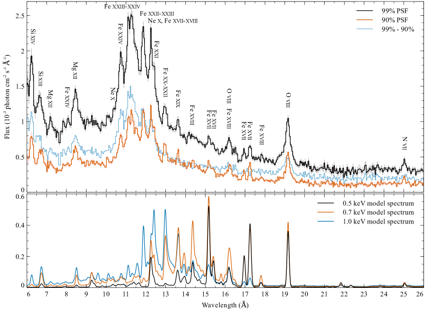
Figure 1: Top panel: fluxed and combined 1st and 2nd order RGS1 and RGS2 data from the two observations. Shown are the spectrum using 95 and 99 per cent of the RGS PSF. Also plotted is the difference between the two spectra, showing the emission from outside of the very central region. The spectra have been binned by a factor of 4 to have 0.04Å spectral bins. Bottom panel: smoothed apec Solar model spectra for gas at 0.5, 0.7 and 1 keV with arbitrary normalisation.

We processed the two source datasets listed in Table 1 using XMM Science Analysis System (sas) version 7.1.0, with the rgsproc pipeline. We processed the 1st and 2nd order spectra, including 99 per cent of the point spread function (PSF) and 97 per cent of the pulse-height distribution, in order to get as many source photons as possible without increasing background too much. We examined the observation light-curves for CCD number 9 at absolute values of the cross dispersion greater than $1.5\times 10^{-4}$ (using values of FLAG of 8 and 16). The lightcurves were relatively consistent at values of around $0.1\hbox{$\rm\thinspace s^{-1}\,$}$, except for some short flaring in the longer observation. We filtered this observation, excluding time periods with count rates greater than $0.2\hbox{$\rm\thinspace s^{-1}\,$}$.

Centaurus fills the entire field of view of the RGS instruments. We therefore required blank-sky background spectra to subtract instrumental and external backgrounds. As we used a 97 per cent pulse-height distribution cut we could not use that standard rgsbkgmodel tool. Instead we selected five deep RGS observations of point-like sources from relatively low Galactic latitude to generate background spectra (Table 1). We processed these observations with the same parameters as Centaurus, cleaning flares in the same way, and excluding the inner 90 per cent PSF (where the sources lie) to generate the background spectra.

We combined with rgscombine the separate background observations to make RGS 1 and RGS 2 spectra for the two spectral orders. We used rgscombine to add the spectra and responses from the two foreground Centaurus observations, after reprocessing including the correct attitude values. The background spectra contained some invalid spectral channels which did not correspond with the foreground spectra, so we marked these channels as invalid in the foreground spectra. We grouped the foreground spectra to have a minimum of 25 counts per spectral bin.

We checked the background spectra were the same by applying them to the foreground individually. The backgrounds were indistinguishable in the 6.5 to 27 Å range.

Table 1: XMM-Newton RGS observations of the target (Centaurus) and the five background fields. RA and Dec are the boresight pointing coordinates, length specifies the observation length, and the exposure is the RGS1 exposure after cleaning for bad time periods (we total 158 and 157 ks exposure on the target in the RGS1 and 2, respectively). $N_{\mathrm{H}}$ shows the weighted Galactic Hydrogen column density towards the object (Kalberla et al., 2005).

XMM observation ID	Target	RA (J2000)	Dec (J2000)	Date	Length (ks)	Exposure (ks)	$N_{\mathrm{H}}$ ($10^{20}\hbox{$\rm\thinspace cm^{-2}\,$}$)
0046340101	Centaurus cluster	$12^{\mathrm{h}}48^{\mathrm{m}}47.93^{\mathrm{s}}$	$-41^{\circ}18^{\prime}43.5^{\prime\prime}$	2002-01-03	47.8	46.5	8.56
0406200101	Centaurus cluster	$12^{\mathrm{h}}48^{\mathrm{m}}43.05^{\mathrm{s}}$	$-41^{\circ}18^{\prime}42.5^{\prime\prime}$	2006-07-25	124.3	111.7	8.56
0112210201	NGC 3783	$11^{\mathrm{h}}39^{\mathrm{m}}01.70^{\mathrm{s}}$	$-37^{\circ}44^{\prime}08.8^{\prime\prime}$	2001-12-17	137.8	72.5	9.91
0112210501	NGC 3783	$11^{\mathrm{h}}39^{\mathrm{m}}01.73^{\mathrm{s}}$	$-37^{\circ}44^{\prime}08.7^{\prime\prime}$	2001-12-19	137.8	124.2	9.91
0300430101	NGC 3256	$10^{\mathrm{h}}27^{\mathrm{m}}51.45^{\mathrm{s}}$	$-43^{\circ}54^{\prime}14.0^{\prime\prime}$	2005-12-06	134.0	116.6	9.14
0302850201	MCG-5-23-16	$09^{\mathrm{h}}47^{\mathrm{m}}45.43^{\mathrm{s}}$	$-30^{\circ}56^{\prime}57.6^{\prime\prime}$	2005-12-10	131.2	111.7	8.69
0305310101	EC 13471-1258	$13^{\mathrm{h}}49^{\mathrm{m}}52.17^{\mathrm{s}}$	$-13^{\circ}13^{\prime}36.0^{\prime\prime}$	2006-01-27	119.4	94.6	5.34

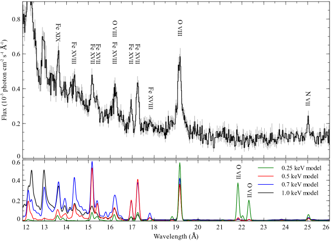
Figure 2: Top panel: fluxed and combined 1st and 2nd order RGS1 and RGS2 data, using 90 per cent of the RGS PSF. The spectrum has been binned by a factor of 2 below 20Å (giving 0.02Å bins) and 3 above that. Bottom panel: smoothed solar-abundance model apec spectra at 0.25, 0.5, 0.7 and 1 keV with arbitrary normalisation.

3 Spectrum

We show in Fig. 1 the full fluxed spectrum using the 99 per cent PSF with 97 per cent of the pulse-height distribution. A 99 per cent PSF corresponds to roughly the inner 160 arcsec width in the cross-dispersion direction. This was created by combining the first and second order spectra for both observations together with the task rgsfluxer, subtracting the combined background spectra. We do not show the spectrum at wavelengths longer than 26Å as the background becomes increasingly important. We note that the output from rgsfluxer is for display purposes only. We do not use it to obtain quantitative information.

In the plot we also show the spectrum extracted from the inner 90 per cent of the PSF (which corresponds to around 60 arcsec width in the cross-dispersion direction). In addition we plot the difference between the two spectra, which is equivalent to the spectrum extracted between 60 and 160 arcsec in the cross-dispersion direction. In the lower panel we show smoothed model apec (Smith et al., 2001) spectra for plasmas with Solar metallicity at temperatures of 0.5, 0.7 and 1 keV for comparison. These models are plotted with arbitrary normalisation to have roughly the same range in values. Note that the spectrum also contains lines from gas hotter than 1 keV.

The spectrum shows a variety of emission lines, from N, O, Ne, Mg, Si and Fe in several ionisation states. Most interesting are those lines indicating cool X-ray emitting gas, particularly strong in the 90 per cent PSF spectrum. Fe L lines from Fe xxiv down to Fe xvii are observed. The strong N vii line, in particular, is interesting.

We show a zoom-up of the spectrum between 12 to 26Å from the 90 per cent PSF in Fig. 2. The plot shows we clearly observe several distinct Fe xvii lines. These lines are relatively narrow, indicating that they come from a relatively small region (See Section 3.1). Absent from the spectra is any evidence for O vii emission (which would appear at 21.8 and 22.2Å at this redshift), which is a strong indicator of gas less than 0.2 keV.

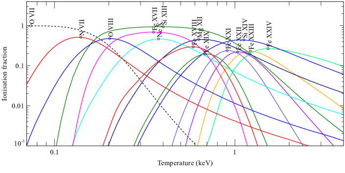
Figure 3: Ionisation equilibrium for lines from observed (solid) and unobserved (dotted) ions as function of temperature in keV (Mazzotta et al., 1998). The data are shown here smoothed with cubic splines.

Different lines are sensitive to gas at different temperatures. The strength of lines from a particular ion are governed by how much of an element is in the form of that ion, the abundance of the element and the density of the gas. We plot in Fig. 3 the fraction of an element which is in the form of a particular ion as a function of temperature, for those ions from which we observe lines (plus O vii which we do not observe). These results are from the calculations of ionisation equilibrium of Mazzotta et al. (1998) (which are used by the apec model).

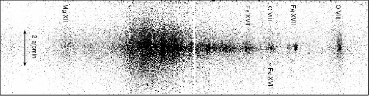
Figure 4: Image of the first order exposure-corrected dispersed spectrum, combining both RGS instruments and observations. The dispersion direction lies along the horizontal axis, with increasing wavelength rightwards. The vertical cross dispersion direction shows a one-dimensional image of the central $\sim 5$ arcmin of the cluster.

We show in Fig. 4 the image formed by plotting the dispersion angle of detected photons against the cross-dispersion angle. Photons outside of the first order spectrum were removed by making an energy-cut using the pulse-invariant CCD energy values. It shows the combined RGS1 and RGS2 cross-dispersion image for the two observations, exposure-corrected for bad pixels. The horizontal axis shows increasing wavelength, while the off-axis angle in the cross-dispersion direction is shown vertically. It can be seen that some lines, e.g. Fe xvii, are much more centrally concentrated than others, e.g. O viii.

3.1 Line cross-dispersion profiles

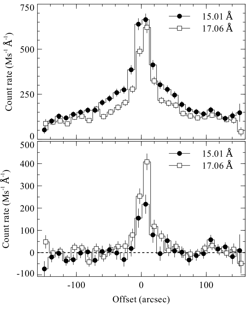
Figure 5: Line profiles as a function of cross-dispersion angle for the two strongest Fe xvii lines. The top and bottom panel shows before and after subtracting neighbouring continuum, respectively.

We can examine this more quantitatively by plotting the profiles of individual lines as a function of cross-dispersion angle. As one of the most interesting cases, we show in Fig. 5 the profiles of the two strongest Fe xvii lines. The 15.01Å line can be strongly resonantly scattered as its oscillator strength is 2.7. Looking at the top panel of Fig. 5, which shows the raw profile in a $\pm 0.1$Å strip either side of the line centre, it appears there is evidence for scattering (a broader 15Å profile). However, subtracting nearby continuum emission creates much more sharply peaked distributions of emission (shown in the bottom panel of Fig. 5), consistent between the two lines. This is much more in line with the predictions from the Chandra Centaurus data of a resonance scattering model (Sanders & Fabian, 2006b), which predicts at most a few per cent effect (resonant scattering is strong in the very central, cool, dense regions, but this cannot scatter radiation to appear to come from a larger radius).

Fitting a Gaussian to the continuum-subtracted profiles gives half energy width (HEW) values of 14.2 and 12.3 arcsec for the 17.06Å and 15.01Å lines, respectively. These values are consistent with the approximate HEW of the RGS mirrors (13.8 and 13.0 for the RGS1 and RGS2, respectively). The 17.06Å blended line strength appears substantially stronger than the 15.01Å signal. We will reexamine this in Section 4.6.

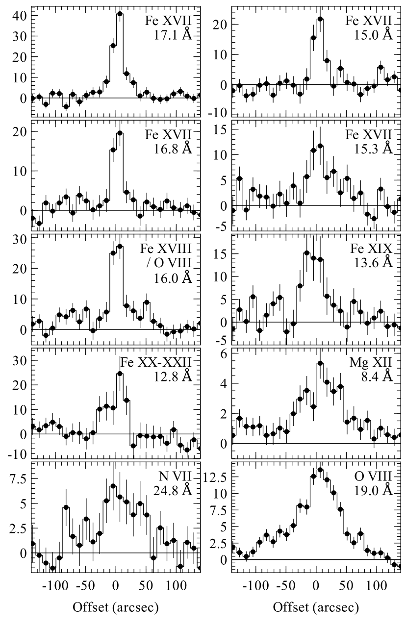
Figure 6: Profiles of several prominent lines in the cross-dispersion direction. The units are in $10^{-5}\>\mathrm{counts}\hbox{$\rm\thinspace s^{-1}\,$}$Å^-1. Continuum has been subtracted from a neighbouring part of the spectrum.

We show in Fig. 6 cross-dispersion profiles of several other strong lines. In each of these cases we plot the profile 0.1Å either side of the centre (except for the broad O viii and Mg xii lines, where we use 0.2Å). The general picture is that lines that are emitted by cooler gas (e.g. Fe xvii, xviii, xix) come from more compact regions. One line which differs from this picture is the N vii line, which is fairly broad in the cross-dispersion profile. Fig. 1 however shows that most of the contribution to this line comes from the inner 90 per cent of the PSF.

4 Spectral fitting

Table 2: Spectral fit results to the data extracted from the 99 per cent PSF aperture. If two or more results are given, this means the parameter was allowed to vary independently in each component, otherwise they were tied together. Upper limits are $2\sigma$. For the multi-temperature models the number in brackets signify the temperature component number the best fitting parameters apply to. The values of the source sizes are HEW, exclusive of the 13.2 arcsec component from the mirrors.

Model	vapec+vapec	vapec+vmcflow k$T_{\mathrm{min}}=0.08\rm\thinspace keV$	vapec+vmcflow k$T_{\mathrm{min}}$ free	$5\times$vapec	$5\times$vmcflow
k$T$ (keV)	$1.85\pm 0.02$ $0.766\pm 0.008$	$1.86\pm 0.02$	$2.04\pm 0.02$ $0.54\pm 0.01$	3.2, 2.4, 1.6, 0.8, 0.4	3.2-2.4, 2.4-1.6, 1.6-0.8, 0.8-0.4, 0.4-0.0808
$N_{\mathrm{H}}$ ($10^{20}\hbox{$\rm\thinspace cm^{-2}\,$}$)	$10.1\pm 0.2$	$10.1\pm 0.2$	$9.7\pm 0.2$	$9.0\pm 0.2$	$8.8\pm 0.2$
sizes (arcmin)	$1.12\pm 0.03$ $0.32\pm 0.03$	$1.19\pm 0.03$ $0.37\pm 0.03$	$1.42\pm 0.04$ $0.35\pm 0.02$	$1.96\pm 0.09$ (1-2), $0.56\pm 0.03$ (3), $0.39\pm 0.04$ (4-5)	$\sim 3$ (1), $0.99\pm 0.04$ (2), $0.32\pm 0.06$ (3), $0.49\pm 0.09$ (4-5)
N	$<0.18$ $3.8^{+0.5}_{-0.8}$	$<0.18$ $0.86\pm 0.12$	$<0.21$ $2.0\pm 0.3$	$<0.15$ (1-2) $1.6\pm 0.2$ (3-5)	$<0.18$ (1-2) $3.5\pm 0.6$ (3-5)
O	$0.32\pm 0.02$ $0.41\pm 0.09$	$0.34\pm 0.02$ $0.15\pm 0.03$	$0.40\pm 0.03$ $0.34\pm 0.05$	$0.47\pm 0.02$	$0.52\pm 0.02$
Ne	$0.45\pm 0.03$	$0.37\pm 0.02$	$0.56\pm 0.04$	$0.74\pm 0.04$	$0.80\pm 0.05$
Mg	$0.60\pm 0.03$	$0.49^{+0.03}_{-0.02}$	$0.69\pm 0.05$	$0.91\pm 0.05$	$1.02\pm 0.07$
Si	$1.22\pm 0.06$	$1.02\pm 0.06$	$1.34\pm 0.05$	$1.60\pm 0.09$	$1.76\pm 0.12$
Ca	$2.0\pm 0.3$	$2.2\pm 0.3$	$2.1\pm 0.2$	$2.6\pm 0.4$	$2.8\pm 0.5$
Fe	$0.66\pm 0.02$ $0.53\pm 0.04$	$0.67\pm 0.02$ $0.29\pm 0.03$	$0.82\pm 0.03$ $0.59\pm 0.07$	$0.97\pm 0.02$	$1.08\pm 0.02$
Ni	$1.81\pm 0.08$	$1.67\pm 0.07$	$1.95\pm 0.09$	$2.34\pm 0.11$	$2.54\pm 0.15$
norm	$(4.14\pm 0.04)\times 10^{-2}$ $(2.0\pm 0.1)\times 10^{-3}$	$(3.89\pm 0.07)\times 10^{-2}$	$(3.46\pm 0.06)\times 10^{-2}$	See Fig. 10	–
$\dot{M}$ ($\hbox{$\rm\thinspace M_{\odot}$}\rm\thinspace yr^{-1}\,$)	–	$7.4\pm 0.5$	$8.7\pm 0.5$	–	See Fig. 12
$\chi_{\nu}^{2}$	$6435/5068=1.27$	$6494/5069=1.28$	$6381/5068=1.26$	$6362/5069=1.26$	$6397/5069=1.26$

The observed spectrum is affected by several factors, listed below.

1. The temperature of the observed region affects the ratio of the strengths of the emission lines and the continuum. Emission lines are increasingly important below $\sim 1$ keV. Some lines, e.g. Fe xvii, are only emitted over certain restricted temperature ranges (see Fig. 3). The spectrum will be the sum of several temperature components which means care must be taken in using line ratios as temperature diagnostics.

2. The metallicity of a temperature component affects the strength of its emission lines. In general the metallicity of each element in the plasma can vary as a function of temperature and position.

3. The spatial size of the emitting region causes spectral broadening. If a temperature component comes from a smaller spatial region, its lines will be broadened less than a component from a large region. Lines are broadened by (Brinkman et al., 1998)

   $$\Delta\lambda=\frac{0.124}{m}\Delta\theta\>\textrm{\AA},$$ (1)

   where $\Delta\theta$ is the source extent (HEW; half energy width) in arcmin, and $m$ is the spectral order. The XMM RGS response already takes account of the broadening for point sources, so this width is on top of the $\sim 13.2$ arcsec HEW PSF of the mirror modules of the RGS.

4. The sensitivity of the RGS is a function of the position on the sky. It is less sensitive to components observed from off axis.

Therefore a complex source like the core of the Centaurus cluster would require a significant amount of modelling to account for each of these effects. There are also degeneracies when fitting the spectra. For example, the emission measure of low temperature gas is inversely proportional to its metallicity as the continuum is difficult to measure.

Our general technique in this paper is to fit multiple thermal models to the spectrum extracted from the RGS. Each thermal model is smoothed by a variable-width Gaussian (of width in wavelength given in equation 1) to take account of the spatial distribution (which assumes the emission region is Gaussian in shape, centred on the cluster centre). We tie the abundances of each of the thermal components together, unless the data are good enough to constrain them in individual components. The thermal components are absorbed by Galactic absorption before smoothing with the Gaussian model.

Our modelling assumes that each component has a fixed temperature, metallicity and spatial scale. In most of the spectral fits we make assumptions in our choice of which parameters to vary. For example, we do not allow many of the metallicities to vary with temperature.

We fitted the first-order spectra between 6.5 and 27Å, where the background is low relative to the foreground. The second-order spectra were fitted between 7 and 15.5Å. xspec version 12.3.1 (Arnaud, 1996) was used to do the spectral fitting. We use the spectra extracted from the 99 per cent PSF to get as complete a picture as possible.

4.1 Single temperature model

To demonstrate that an isothermal model is inadequate, we show in Fig. 7 the best fitting single temperature vapec (Smith et al., 2001) model. In this model the temperature, Galactic column density and normalisation are free. The relative normalisations of each RGS dataset are allowed to vary relative to the RGS1 first order spectrum. The N, O, Ne, Mg, Si, Ca, Fe and Ni metallicities are free to vary. The spectrum is smoothed by a variable-width Gaussian to account for spatial broadening of the spectral lines (Equation 1). The 1.6 keV model fails to account for the Fe xvii and N vii lines ($\chi^{2}_{\nu}=7474/5075=1.47$).

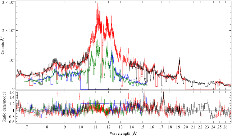
Figure 7: Best fitting single-temperature model and ratio of data to model for the 99 per cent PSF spectra. The points are the first and second order data from the two RGS detectors and the lines are the best fitting model after folding through the response. The data have been rebinned for display in xspec to have a signal to noise ratio of 13. The model fails to account for the Fe xvii and N vii lines.

4.2 Simple two-temperature model

The most simple extension of a single thermal component model is one with two temperature components. This model consists of two vapec components, each with a variable temperature, normalisation, and N, O and Fe metallicities. They are absorbed by the same Galactic column density, but are allowed to vary independently in spatial size (smoothing according to Equation 1). The Ne, Mg, Si, Ca and Ni metallicites are tied between the two components and allowed to vary independently. We allow the N metallicity to vary between the two components because the N vii line is narrow. If the hot component is forced to have the same N metallicity as the cool component, then the model cannot fit the narrow line because too much emission comes from larger spatial regions. Table 2 shows the best fitting values of each of the parameters and their uncertainties. The improvement in $\chi^{2}$ is around 1000 over the single temperature model. The best fitting temperatures, 0.77 and 1.85 keV, are very close to the range of values found in the inner arcmin by Chandra (Fabian et al., 2005).

The best fitting iron metallicities, however, are substantially lower than the $1.5-2\hbox{$\thinspace\mathrm{Z}_{\odot}$}$ peak values from Chandra and XMM CCD spectra (Sanders & Fabian, 2006a). In fact all of the metallicities (except Ca) of each of the elements we measure from the RGS spectra are significantly lower than the CCD results. CCD measurements indicate that the metallicities drops dramatically in the innermost region (Sanders & Fabian, 2002), which may correspond with this low metallicity. We will discuss this further in Section 5.4.

The lines from cooler temperature gas are narrower than the lines from hotter gas, leading to a larger spatial scale for the hot component (1.1 vs 0.3 arcmin). The emission measure of the cooler component is only around 5 per cent of the hot component.

4.3 Multi-temperature model

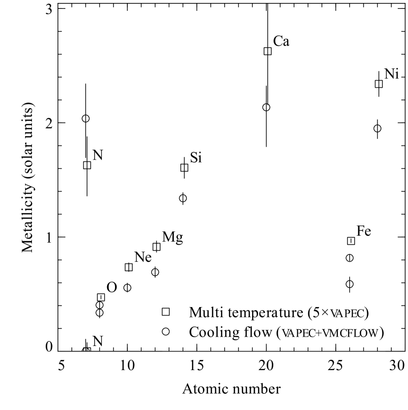
Figure 8: Best fitting metallicities for the spectral fits from multi-temperature ($5\times$vapec) and cooling flow model fits (vapec+vmcflow with free minimum temperature) to the data extracted from the 99 per cent PSF. Note that N, O and Fe are allowed to vary between the two components in the vapec+vmcflow model.

Figure 9: Best fitting spatial size of spectral fits using the line widths for the $5\times$vapec model (adding the PSF contribution). The lines connect temperature components which have their sizes tied together.

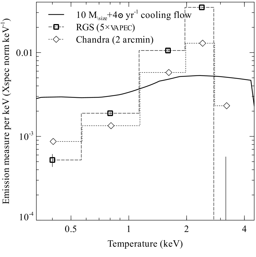
Figure 10: Comparison of the RGS with Chandra emission measures per unit temperature as a function of temperature. The Chandra results were extracted from a 2 arcmin radius around the core of the cluster. The solid line shows the expected distribution of emission measure for a $10\hbox{$\hbox{$\rm\thinspace M_{\odot}$}\rm\thinspace yr^{-1}\,$}$ isobaric cooling flow at Solar metallicity, cooling from a temperature of 4.5 keV to 0.0808 keV using the mkcflow model.

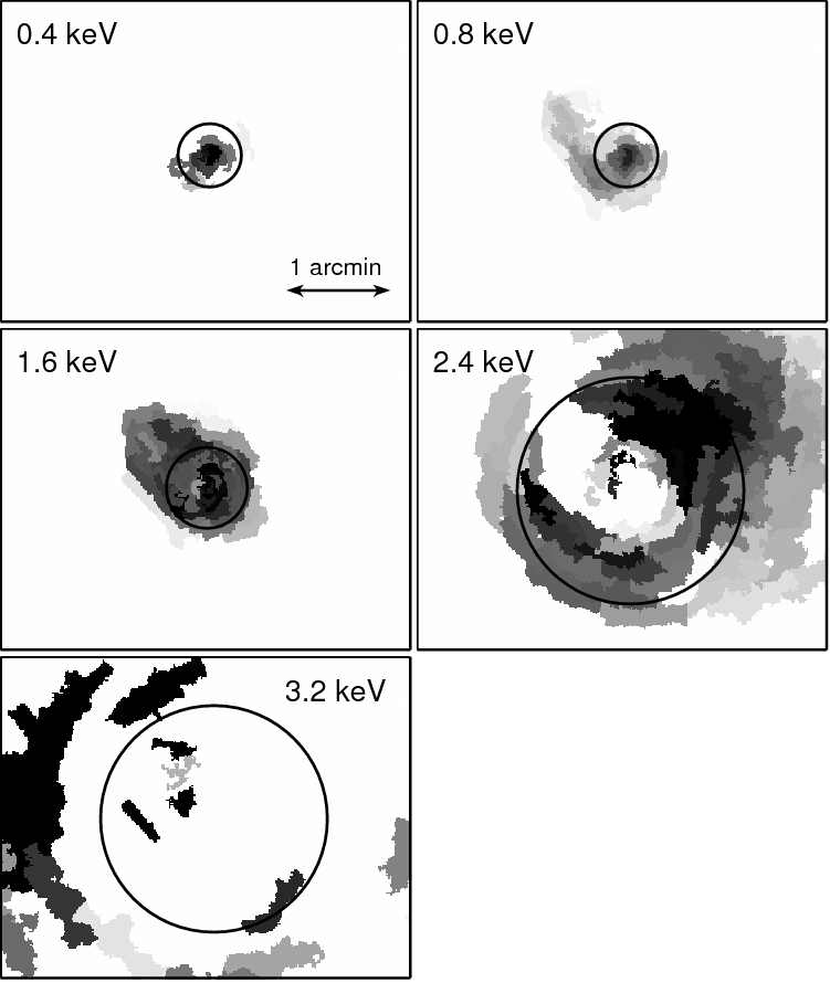
Figure 11: Maps of the Chandra emission measure per unit area using multi temperature model. The circles show the best fitting HEW of the emission from the line widths in the spectral fits to the RGS data (the 0.4 and 0.8 keV components are forced to be equal, as are the 2.4 and 3.2 keV components), including the effect of the PSF. The RGS cross-dispersion direction for the longer observation lies along the cool plume.

We can extend the two-temperature model with more temperature components. Multitemperature fits with several free temperatures typically become unstable when spectral fitting. To avoid this we constructed a model containing components with fixed temperatures, allowing the emission measure of each component to vary. We used a multi-temperature model containing five components ($5\times$vapec). We used a range of temperatures in the model to account for the ranges of temperatures in the cluster the spectrum is sensitive to, with components at 0.4, 0.8, 1.6, 2.4 and 3.2 keV. We also tried an 8 component model, but the quality of the fit was only slightly improved and it was difficult to constrain the parameters.

Table 2 show the best fitting parameters for these two models. To reduce the number of free parameters, we only used a single set of metallicities for the temperature components (tieing O, Ne, Mg, Si, Ca, Fe and Ni). We however split the components by temperature to allow for two N values, otherwise there are obvious residuals around the N vii line. Rather than allow the spatial scale of each of the components to vary, or fixing them to be all the same, we apply three different spatial smoothing scales to groups of the temperature components.

We plot the abundance of each variable relative to solar in Fig. 8 for the $5\times$vapec model. In Fig. 9 is shown the best fitting HEW sizes from the line widths against the temperature of the component. We note that velocity broadening of the lines could mimic spatial broadening, however, velocities above $700\hbox{$\rm\thinspace km\rm\thinspace s^{-1}\,$}$ are required to make a substantial difference to these measurements.

The emission measure of each component per unit temperature (assuming a temperature bin size which is half the logarithmic change to the next adjacent temperature value) is plotted as a function of temperature in Fig. 10. In this plot we also show values from a Chandra spatially-resolved analysis of the inner 2 arcmin. These were created from spectra extracted from contour-binned (Sanders, 2006) regions containing around $\sim 10^{4}$ counts. The spectra were fit with a multi-temperature $5\times$apec model with the same five fixed temperatures as the RGS fit, but assuming Solar abundance ratios. The model assumes each temperature component in individual regions has the same metallicity.

The RGS and Chandra results are roughly similar, considering we are comparing the Chandra results in the inner 2 arcmin radius with the larger field of view of the RGS instruments and the decline of the RGS effective area off-axis. The one major discrepancy is the apparent lack of any gas above 3 keV in the RGS results (see Section 5.4 for a discussion). We also plot the HEW size from the line widths on the Chandra emission measure maps on Fig. 11, showing they are comparable.

The solid line in Fig. 10 shows the expected distribution of emission measure for a simple isobaric cooling flow, cooling at the rate of $10\hbox{$\hbox{$\rm\thinspace M_{\odot}$}\rm\thinspace yr^{-1}\,$}$ without any heating. It can be seen that the observed emission measure of gas decreases more steeply with temperature than predicted by a simple cooling flow.

4.4 Single cooling flow component

We have investigated how well the observed spectrum can be modelled by a simple cooling flow. Our first model was based on a vapec component plus a vmcflow cooling flow component. We used the new feature in xspec version 12 to base the cooling flow model spectrum on a apec thermal model rather than a mekal one. We note, however, that this form of the model is not internally self consistent, as the quantity of gas at each temperature is computed by assuming the luminosities of the mekal model. We made our own consistent version of the model, but this had no effect on the predicted spectrum, so we show results from the xspec model here.

We tried two forms of the model: a full cooling flow where the lower temperature of the cooling flow was constrained to be the minimum possible (0.0808 keV) and the second reduced model where it was allowed to be a free parameter. In this model we allowed the N, O and Fe metallicites to vary between the vapec and vmcflow components, but fixed the other metallicities to have the same values in the two components.

The best fitting parameters for the two models are shown in Table 2. The full cooling flow model gives a mass deposition rate of $7.4\pm 0.5\hbox{$\hbox{$\rm\thinspace M_{\odot}$}\rm\thinspace yr^{-1}\,$}$, whereas the reduced model obtained a rate of $8.7\pm 0.5\hbox{$\hbox{$\rm\thinspace M_{\odot}$}\rm\thinspace yr^{-1}\,$}$ cooling to $0.54\pm 0.01\rm\thinspace keV$. The metallicities of the cooling flow component were lower for the model where the gas cools to the minimum value, presumably to decrease the strength of the emission lines.

The reduced cooling flow model gives a substantially better quality of fit to the spectrum than the full model ($\chi^{2}=6381$ versus 6494), but is poorer than the five component multitemperature model ($\chi^{2}=6362$).

4.5 Multiple cooling flow components

Figure 12: Mass deposition rates in the absence of heating using a cooling flow model made up of five different temperature ranges ($5\times$vmcflow).

A simple cooling flow is unlikely to be a good model to the complex distribution of gas in the core of the Centaurus cluster, even in the presence of cooling gas. We have therefore used a model where the cooling flow is split into different temperature ranges and we allow the mass deposition rate to vary in each range. We use fixed ranges in temperature to obtain a stable fit. The model examined here has steps in temperature from 3.2 to 2.4, 2.4 to 1.6, 1.6 to 0.8, 0.8 to 0.4 and 0.4 to 0.0808 keV. The metallicities are assumed to be the same in each component, except for the N metallicity in the three coolest components, which is allowed to vary separately from the hotter components.

We show in Fig. 12 the mass deposition rate in the absence of heating for each of the cooling flow components. We measure mass deposition rates down to 0.4 keV and an upper limit of $0.8\hbox{$\hbox{$\rm\thinspace M_{\odot}$}\rm\thinspace yr^{-1}\,$}$ below that temperature. The results are consistent with the multitemperature model results. There is systematically less gas detected at lower temperature than expected from a simple cooling flow (as in Fig. 10).

4.6 Direct spectral line measurements

Table 3: Line luminosities for some of the more interesting lines. The listed wavelengths are rest wavelengths, averaging the position of lines in blends. The temperature range is the approximate range in temperature of gas the lines are emitted from (where the emissivity is within an order of magnitude of the peak). The widths are measurements of the Gaussian width, upper limits ($2\sigma$) or fixed at 0. The power and mass deposition rates are corrected for Galactic absorption. The mass deposition rates are calculated assuming a cooling flow cooling to 0.0808 from 4.5 keV temperature with Solar metallicities.

Line	Wavelength (Å)	Temperature range (keV)	Width (Å)	Power ($10^{39}\hbox{$\rm\thinspace erg\rm\thinspace s^{-1}\,$}$)	$\dot{M}$ ($\hbox{$\rm\thinspace M_{\odot}$}\rm\thinspace yr^{-1}\,$)
Fe xvii	15.01	$0.2\rightarrow 0.9$	$<0.07$	$12.4\pm 1.5$	$1.6$
Fe xvii	15.26	$0.2\rightarrow 0.9$	$0$	$3.6\pm 1.3$	$1.6$
Fe xvii	16.78	$0.2\rightarrow 0.9$	$0$	$4.3\pm 1.2$	$1.7$
Fe xvii	17.06	$0.2\rightarrow 0.9$	$0.047\pm 0.009$	$19.3\pm 2.0$	$3.0$
N vii	24.78	$<0.85$	$0.050\pm 0.014$	$11.5\pm 1.6$	$9.7$
O vii	21.60	$<0.4$	$0$	$<4.6$	$<3.4$
O vii	22.10	$<0.4$	$0$	$<7.7$	$<2.9$

Instead of direct spectral fitting to the whole of the spectrum, the strength of the emission lines can be used to gauge the amount of cooling taking place through the temperature range they are sensitive to. The amount of flux in a line can be compared to that expected from a cooling flow model. As there are several possible lines which can be examined, this allows independent determinations of the mass deposition rate, but does not use the full spectral information available when spectral fitting.

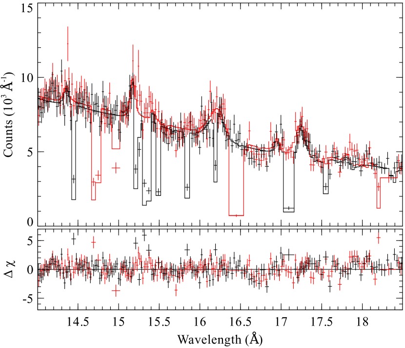
Figure 13: Absorbed powerlaw plus Gaussians model fit to the Fe xvii region of the spectrum. The top panel shows the background-subtracted data and best fitting model. The bottom panel shows the contribution, $\Delta\chi$, of each channel to $\chi^{2}$. The RGS1 and RGS2 data and models are shown in black and red, respectively. The spectrum has been rebinned to a signal-to-noise ratio of 10 in xspec.

4.6.1 Fe xvii

To examine the Fe xvii line powers we fitted a spectral model made up of an absorbed powerlaw plus Gaussians, fitted to the first order spectra between 14 and 18.5Å extracted from 99 per cent of the PSF. We used a Gaussian for each of the distinct Fe xvii lines (Table 3), two Gaussians at 16.07 and 16.00Å for Fe xviii and O viii, and Fe xviii Gaussians at 14.21Å and 17.62Å. The strong lines at 15.01, 16.00, 16.07, and 17.06 were allowed to have variable widths. The other lines were fixed at zero width. Galactic absorption was fixed at $8.56\times 10^{20}\hbox{$\rm\thinspace cm^{-2}\,$}$.

Table 3 shows the best fitting widths and de-absorbed line luminosities. Fig. 13 shows the data with best fitting model. The line powers would be increased if there were any internal absorption within the cluster (as suggested by Crawford et al. 2005 and Sanders & Fabian 2006b). We convert these powers into mass deposition rate by comparing them against the expected flux from a cooling flow model. This was done by firstly simulating a high signal-to-noise spectrum using a $10\hbox{$\hbox{$\rm\thinspace M_{\odot}$}\rm\thinspace yr^{-1}\,$}$ vmcflow model, cooling between 4.5 and 0.0808 keV, with Solar abundance, absorbed with Galactic absorption. We then measured the fluxes in the simulated lines by fitting the same absorbed powerlaw plus Gaussian model as we did to the data. The ratio of the line flux in the data compared to the simultated model was used to obtain a mass deposition rate. Note that the assumed relative abundance can make a substantial difference to these values. The mass deposition rates obtained for three of the lines agree at $\sim 1.6\hbox{$\hbox{$\rm\thinspace M_{\odot}$}\rm\thinspace yr^{-1}\,$}$, but the 17.06Å blended line is substantially stronger than the others.

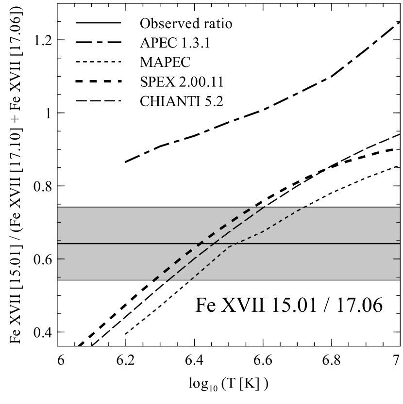
Figure 14: Predicted ratio of the 15.01 line to the blended 17.06 line as a function of temperature for a variety of different plasma codes. The line with surrounding shaded region shows the best fitting value and its uncertainty.

The apec model predicts that the 15.01Å line should be more powerful than the 17.06Å blended line over a wide range of temperatures. However in our data the 17.06Å lines are 56 per cent brighter than the 15.01Å line. A possible cause for this is resonant scattering, as the 15.01Å transition is resonant with a large oscillator strength. If this were the case the scattered radiation would have to be absorbed, as scattering only increases the spectral width of the line, redistributing the flux.

However, a likely reason for the discrepancy in brightness may be due to uncertainties in spectral models. We plot in Fig. 14 the predicted ratio of the 15.0 to blended 17.0Å lines versus the temperature for some different plasma codes, including apec, mapec (modified apec results using a many-body perturbation theory method to calculate new values for the emissivities of Fe and Ni L-shell lines; Gu 2007), spex (the latest mekal results from the spex package; Kaastra & Mewe 2000) and chianti (Dere et al., 1997; Landi et al., 2006).

It appears apec cannot reproduce the observed line ratio (as found by Xu et al. 2002). The other plasma codes are able to and agree fairly well. The line ratio appears to indicate that the Fe xvii line emission comes from an average temperature of $0.25^{+0.20}_{-0.09}\rm\thinspace keV$. Note that although apec appears to fit the data worse here, its quality of fit to the total spectra is at least $\Delta\chi^{2}\sim 300$ better than the spex mekal model overall.

The Fe xvii 17.06Å line width of 0.047Å translates into a HEW of 36 arcsec (including the effect of the mirrors). This is larger than the width of the emission line in the cross-dispersion direction (Fig. 5; compatible with the PSF). The longer observation analysed here has the cross-dispersion direction placed along the plume. The difference in source extent between the line widths and cross-dispersion profiles may be due to the very coolest gas being extended in the direction perpendicular to the cross-dispersion direction (Fig. 11; Crawford et al. 2005).

If a cooling flow model plus powerlaw continuum is fit to this region of the spectra containing the Fe xvii lines, the best fitting mass deposition rate is $1.90\pm 0.13\hbox{$\hbox{$\rm\thinspace M_{\odot}$}\rm\thinspace yr^{-1}\,$}$. This is for a cooling flow at Solar abundance cooling from 4.5 to 0.0808 keV. As the Fe metallicity decreases, the mass deposition rate climbs to $3.8\hbox{$\hbox{$\rm\thinspace M_{\odot}$}\rm\thinspace yr^{-1}\,$}$.

4.6.2 O vii

We next placed upper limits on the O vii lines at 21.6 and 22.1Å. We fitted an absorbed powerlaw to the spectra from 19.5 to 23Å plus two zero-width Gaussians at the line positions. We calculated upper limits for the line powers and converted these to upper limits on the mass deposition rate. These upper limits of $\sim 3\hbox{$\hbox{$\rm\thinspace M_{\odot}$}\rm\thinspace yr^{-1}\,$}$ are compatible with the Fe xvii results, although Solar metallicity is assumed. The O/Fe metallicity will affect these values as Fe is the main coolant in this temperature range (Böhringer & Hensler, 1989).

Figure 15: Flux ratio of 21.60Å O vii ratio to 15.01Å Fe xvii line. The model lines show the ratio as function of temperature for Solar abundance. The horizontal line shows the observed upper limit.

We note that if the emission only came from gas at 0.25 keV, we would expect the O vii lines to be much stronger than Fe xvii (see Fig. 2 lower panel). The relative strength of the Fe xvii and O vii will depend on the metallicity and ionisation balance, however. We show in Fig. 15 the expected ratio of the 21.60Å O vii to 15.01Å Fe xvii line as a function of temperature assuming Solar abundance. The ratio of any of the O vii to Fe xvii lines is a strong function of temperature. For sensible ranges in abundance (O/Fe from 0.3 to 1 Solar), it appears unlikely that the temperature of the material emitting the Fe xvii lines is less than $10^{6.55}-10^{6.6}$ K. O/Fe of around 0.1 Solar is required for 0.25 keV material to be consistent with the line ratio. This means a likely lower temperature is $0.3-0.35\rm\thinspace keV$, still within the allowable range of the Fe xvii ratio. These estimates all assume that the line emission comes from isothermal gas.

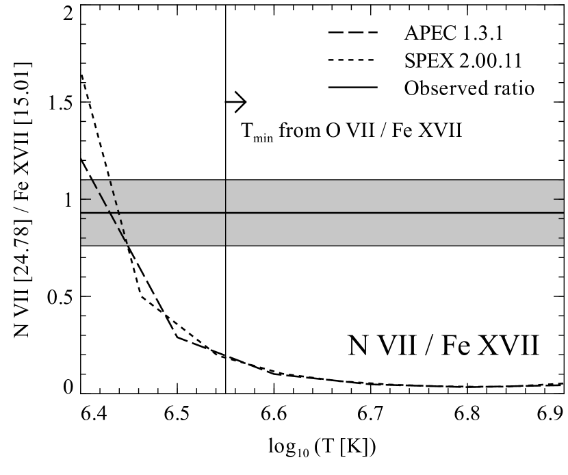
Figure 16: Flux ratio of 24.78Å N vii ratio to 15.01Å Fe xvii line. The model lines show the ratio as function of temperature for Solar abundance. The shaded region shows the observed ratio. The vertical line shows the minimum temperature from the O vii to Fe xvii line ratios (Fig. 15).

We also note that resonant scattering could be important for the 21.6Å Ovii line, which has a high oscillator strength (0.7). Although scattering by itself would not decrease the line flux, it would broaden the spectral line, making it harder to detect. Absorbing material within the scattering region could also reduce the line flux.

4.6.3 N vii

We also try to measure the mass deposition rate in the absence of heating using the N vii line. We fit the region 23 to 30Å with an absorbed powerlaw plus Gaussian with variable width. The power in this line compared to the Fe xvii lines is large: assuming solar abundance its power corresponds to a $10\hbox{$\hbox{$\rm\thinspace M_{\odot}$}\rm\thinspace yr^{-1}\,$}$ cooling flow. This indicates that the N abundance of the cool X-ray emitting gas relative to Fe is large, as was also shown by the spectral fits. Additionally the N vii line covers a larger range in temperature, and so is sensitive to hotter gas which shows a higher effective mass deposition rate (Fig. 12). We note that any additional absorption will increase this line power relative to the Fe xvii lines.

The spectral width of the line is also very close to the Fe xvii 17.06Å line width, meaning it originates from the same spatial region. The finite widths of the lines (a point source would provide an upper limit as the response already takes account of the XMM PSF) show that the emitting region is resolved, with a HEW of around 35 arcsec (taking into account the XMM PSF HEW).

If the lower bound on the temperature is $10^{6.55}$ K, then the ratio of the N xvii to Fe xvii 15.01Å line implies supersolar N abundances (Fig. 16). The minimum N/Fe metallicity as indicated by the apec and spex model line ratios is at least $4\hbox{$\thinspace\mathrm{Z}_{\odot}$}$. This value is in rough agreement with the spectral fitting results.

5 Discussion

5.1 Temperature range

The observed range in temperature of X-ray emitting gas, from 3.7 keV (Sanders & Fabian, 2002) to $\sim 0.35\rm\thinspace keV$ is one of the largest observed up to now in a cluster of galaxies. These RGS results confirm earlier CCD detections of cool gas.

Another cluster with a large apparent X-ray emitting temperature range is the Perseus cluster, containing X-ray emitting filaments at around 0.7 keV in a cluster up to 7 keV (Sanders & Fabian, 2007), although these are clearly influenced by magnetic fields.

The result emphasises that gas certainly does exist at temperatures below the often quoted factor of 2 or 3 in galaxy clusters. Fig. 10 shows that the emission measure of cooler components is progressively smaller than a cooling flow model as the temperature decreases. The lack of detections of cool gas in other clusters using RGS observations could be due to their relatively short exposures, which are typically only 30–40 ks (Peterson et al., 2003).

The large range in temperature in this cluster may be connected to the lack of disruption in its core. The high enrichment of the central parts of the cluster indicates it has been stable for 8 Gyr or more (Sanders & Fabian, 2006a).

5.2 Cooling flow model

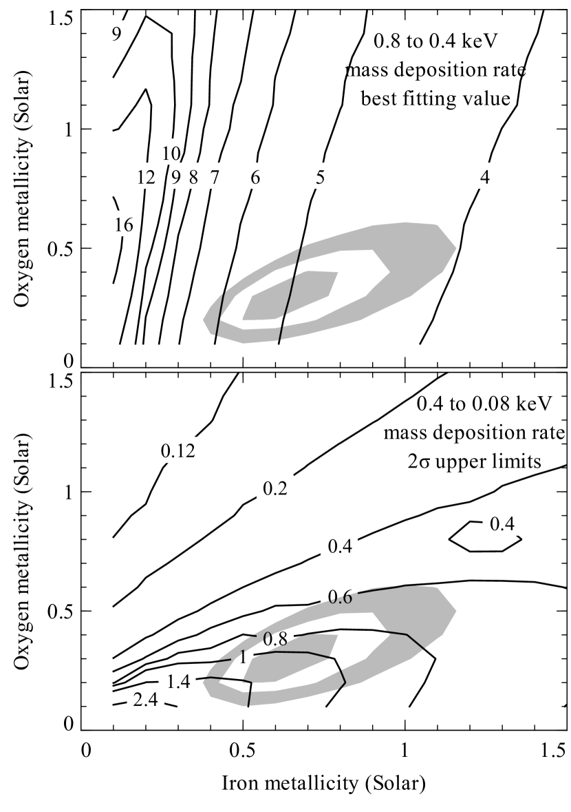
Figure 17: Variation of mass deposition rate with Iron and Oxygen metallicity for the two coolest temperature ranges in Fig. 12. The top panel shows as contour lines the best fitting mass deposition rates in $\hbox{$\rm\thinspace M_{\odot}$}\rm\thinspace yr^{-1}\,$for the 0.8 to 0.4 keV temperature range. The bottom panel shows upper limits for 0.4 to 0.08 keV. Also plotted as shaded regions on both panels are the 1, 2 and 3-$\sigma$ confidence regions for the O and Fe metallicity, calculated using the $\Delta\chi^{2}$ method from the minimum $\chi^{2}$ value.

Figure 18: Variation of mass deposition rate with excess column density above $8\times 10^{20}\hbox{$\rm\thinspace cm^{-2}\,$}$. Shown are the best fitting mass deposition rates in $\hbox{$\rm\thinspace M_{\odot}$}\rm\thinspace yr^{-1}\,$for the 0.8 to 0.4 keV temperature range, or upper limits for the 0.4 to 0.08 keV temperature range.

Fig. 10 and Fig. 12 show that a full simple cooling flow, where gas is cooling by radiative cooling at a constant rate, is not operating in this cluster. However there are some possible reasons why the amount of cold gas may be underestimated:

1. These models assume that there is a fixed metallicity of material as a function of temperature. The O and Fe abundances change the cooling function and strengths of lines significantly. Fig. 17 shows how the mass deposition rate for the $5\times$vmcflow cooling flow model varies as a function of metallicity, for the two coolest temperature ranges. This was made by iterating over a grid of O and Fe abundances and measuring the mass deposition rate at each point. It shows that the real cooling rate is a strong function of metallicity. If the metallicity of the material in the central regions is small there could be significantly more cooling taking place. There is evidence for a drop in metallicity in the central regions (Sanders & Fabian, 2002). This analysis highlights that the best fitting Fe and O metallicities for the two coolest components are small.

   Indeed, O vii emission is the main indicator of cool gas in this waveband, but Fe line emission is actually the main coolant (Böhringer & Hensler, 1989). Therefore the O lines are suppressed if the Fe metallicity is increased while the O metallicity is constant, for a fixed observed Fe xvii strength in a cooling flow. Therefore gas below 0.35 keV can exist without strong O vii emission.

2. Intrinsic absorption could hide much of the cooling taking place. There is evidence that there are large amounts of obscuring material in the core of this cluster (Crawford et al., 2005; Sanders & Fabian, 2006b), where the coolest material resides. It is difficult for spectral fitting to account for this as the continuum is hard to detect for low-temperature gas. We investigated this by fitting the $5\times$vmcflow to the data with varying levels of absorption applied to the two lowest temperature components (note that these results were obtained by varying the absorption separately for each component). In Fig. 18 we plot the increase in mass deposition rate it is possible to obtain by increasing the absorption.

3. The cooling flow model fitted to the data assumes that isobaric (constant pressure) cooling is taking place. If the cooling time becomes shorter than the sound-crossing time, then isochoric (constant density) cooling may be more appropriate. This could also result from the magnetic pressure in clumps becoming dominant as the cooling proceeds. The strength of UV emission lines from isochoric cooling is only around 60 per cent of that expected from isobaric cooling (Edgar & Chevalier, 1986). This would lead to the amount of cooling being underestimated if a cooling flow were taking place. As we show below, the mean radiative cooling time is only $\sim 10^{7}$ yr for the very coolest X-ray detected gas.

4. If the X-ray emitting gas mixes with the cooler optical line emitting material in the very central regions (Crawford et al., 2005), than it will rapidly cool non-radiatively much faster than a cooling flow model would predict (Fabian et al., 2002). The thermal energy is eventually radiated at much longer wavelengths, in the optical/UV/IR filaments, for example, or by dust. There is, indeed, extended mid-IR emission observed from NGC 4696 (Kaneda et al., 2007), which could in part be powered by such a mixing process.

When fitting the data with a cooling flow model, we find progressively smaller mass deposition rates at lower temperatures, as found previously by Peterson et al. (2003). However we detect gas over a much wider range in temperature (a factor of 10 rather than 3) than in their shorter observations, with a wider range of best fitting mass deposition rates (a factor of 50 rather than 10), in reality corresponding to detecting a wider range of emission measures for the temperature components.

Taking gas at 0.35 keV in pressure equilibrium with the gas with $n_{\mathrm{e}}\sim 0.1\hbox{$\rm\thinspace cm^{-3}\,$}$ and $kT\sim 1$ keV (Sanders & Fabian, 2006b), implies a density of this cool material of around $n_{\mathrm{e}}\sim 0.3\hbox{$\rm\thinspace cm^{-3}\,$}$. We can calculate the bolometric luminosity from a unit volume of this material (using the abundances from the $5\times$vapec model) and its internal energy (assuming $\frac{5}{2}\,k_{\mathrm{B}}Tn_{\mathrm{tot}}$). Dividing the two gives a mean radiative cooling time of only $\sim 10^{7}\rm\thinspace yr$ for this 0.35 keV material.

The 0.4 keV component in the $5\times$vapec model is close to 0.35 keV in temperature. Assuming the material is in pressure equilibrium with its surroundings and taking its emission measure from the $5\times$vapec spectral fit, we can estimate it occupies a volume of $2.3\rm\thinspace kpc^{3}$. The region that the Fe xvii lines are emitted from has a radius of at most 10 arcsec, implying a maximum volume of $120\rm\thinspace kpc^{3}$. This means the 0.4 keV material must fill only 2 percent of that very central region. Chandra temperature maps of the core show that the coolest gas is not volume-filling, but exists in the form of cool blobs (Crawford et al., 2005).

5.3 Heating

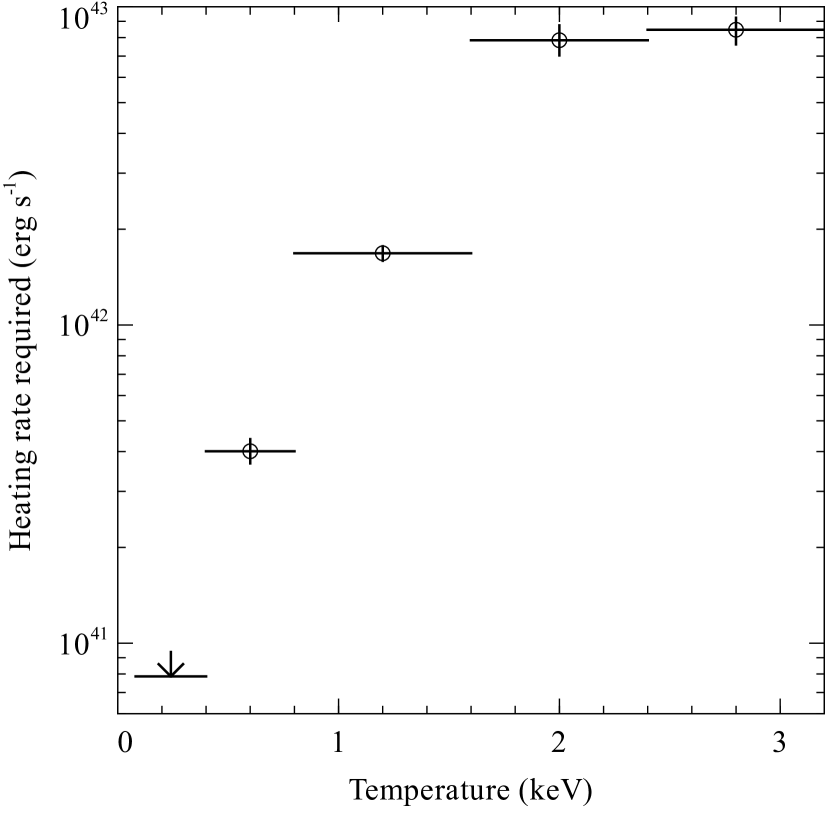
Figure 19: Heating rate required to combat cooling, calculated for each of the individual temperature ranges in the $5\times$vmcflow model (see Fig. 12).

The amount of heating which would be required to offset cooling of the ICM in the cluster can be estimated. We took the $5\times$vmcflow cooling flow model fits to the spectra and generated a chain of parameters using a Markov Chain Monte Carlo. The chain was created with the built-in xspec functionality and was checked for convergence by repeating the analysis with a different starting point. We generated luminosities for each of the sets of parameters in the chain for the individual temperature ranges in the model. We examined the distribution of luminosities to estimate the medians and uncertainties. The luminosities of each temperature range are the rates of heating required to offset cooling.

In Fig. 19 we show the amount of heating required for each temperature range of gas in order to combat cooling. At temperatures of above $\sim 1.5\rm\thinspace keV$, significant heating rates of a few times $10^{43}\hbox{$\rm\thinspace erg\rm\thinspace s^{-1}\,$}$ are required. For the coolest gas it is likely that mixing and conduction complicate this picture. The cool gas we observe here must exist as distributed clumps and the short radiative cooling time places constraints on heating models.

5.4 Metallicity of the gas

The best fitting metallicities we measure show some model dependence. Those models with larger number of temperature components tend to have higher metallicites. However there is quite good agreement between the ratios of the various elements between the best fitting models here and with the previous CCD results.

The metallicities we measure here are smaller than the peak values obtained using CCD data from Chandra and XMM (Sanders & Fabian, 2006a). It is however difficult to compare them exactly as the CCD results are spatially-resolved and the metallicity appears to rise to high values, but drops in the very central region. The temperature is also declining towards the centre. Over the region examined by the RGS detectors, it is likely that there is a rise in metallicity with radius.

Ni shows significantly smaller metallicities of around $2.4\hbox{$\thinspace\mathrm{Z}_{\odot}$}$ here when compared to earlier Chandra and XMM spatially-resolved CCD results (which peak near $4\hbox{$\thinspace\mathrm{Z}_{\odot}$}$; Sanders & Fabian 2006a). This can be mostly resolved by allowing the Ni to vary between the coolest and hotter components, obtaining values of $3.5^{+0.5}_{-0.4}$ and $1.7_{-0.1}^{+0.2}\hbox{$\thinspace\mathrm{Z}_{\odot}$}$, respectively (for the $5\times$vapec model). This highlights that the assumptions or choices we made in modelling the data can have a large impact on the obtained quantities.

The generally smaller metallicites we find here, when compared to CCD results, may be due to problems modelling the continuum from hot gas outside of the central region. Fig. 10 shows that the RGS results require very little hot gas in the spectral fits when compared to Chandra. If we add the expected 3–4 keV hot component from the Chandra spectral fits to the RGS spectral models, freezing its emission measure to the same value, then we typically find the metallicities we measure are increased by 30 to 40 percent. The RGS spectra appear to require much less of this hot material than all previous analyses. Therefore there may be calibration uncertainties at short wavelengths in the RGS spectra.

Another possible reason for higher continuum, leading to underestimates of the metallicity, would be the previously observed non-thermal emission (Allen et al., 2000; Di Matteo et al., 2000). The sedimentation of helium in the core of the cluster would also lead to higher continuum (Ettori & Fabian, 2006).

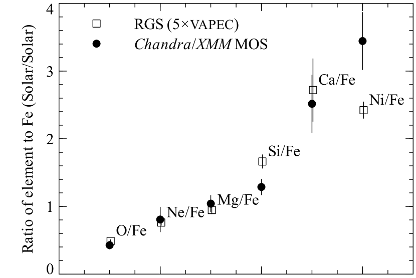
Figure 20: Ratio of metallicity of elements to Fe obtained from the RGS data with the $5\times$vapec model, compared to the results from the central regions of the cluster from combined Chandra and XMM EPIC MOS data (Sanders & Fabian, 2006a).

The ratio of elemental abundances is likely to be more robust than measurements of individual abundances. In Fig. 20 we plot the ratio of the metallicity of various elements to Fe (the ratios are $\hbox{$\thinspace\mathrm{Z}_{\odot}$}/\hbox{$\thinspace\mathrm{Z}_{\odot}$}$), measured using the multitemperature $5\times$vapec model (Fig. 8). Also shown are the same ratios obtained from Chandra and XMM EPIC MOS data. These were calculated by averaging the central XMM and Chandra East and West points from figure 15 (bottom panel) in Sanders & Fabian (2006a). The plot shows that we get good agreement between the RGS, and previous CCD ratios within the inner 10 kpc radius, with some discrepancy for Si/Fe and Ni/Fe. These results indicate that the CCD-derived metallicity ratios in Sanders & Fabian (2006a) are robust.

If the coolest gas is examined separately from the hotter gas, it appears to have lower Fe and O metallicity, confirming the central abundance drop in the spatially resolved CCD measurements. Fig. 17 shows the best-fitting values of the cooler gas are only around 60 per cent of the metallicity of the hotter gas.

It is possible that the metallicity variations are with temperature, not radius, although we do not understand why. If there is a continued decrease of metallicity as temperature decreases then the low O vii result might be understood. It is unlikely that the low metallicity gas can be introduced into the centre, and we presume that the metals are removed. At a temperature of 0.2 keV the cooling rate is sensitive to the metallicity. One simple explanation is that the high metallicity gas is inhomogeneous, conduction is suppressed between clumps, leading to the the high metallicity regions cooling out (Morris & Fabian, 2003). This means that both the injection of metals is a inhomogeneous process and the metals remain poorly mixed for a considerable time (several Gyr).

We measure values for the N abundance of between 1.6 (from the $5\times$vapec model) to $4\hbox{$\thinspace\mathrm{Z}_{\odot}$}$ (for the $5\times$vmcflow and lower limit from the line ratios).

The nitrogen emission lines in the optical spectrum of the emission-line filamentary nebula in NGC 4696, the central galaxy in the Centaurus cluster also indicate a high nitrogen abundance. Specifically, the [NII]/H$\alpha$ line ratio found by Johnstone et al. (1987) of 3.2 is higher than the ratio of less than two which can be accounted for by photoionization or shock models for a solar abundance plasma (Heckman et al., 1989; Voit & Donahue, 1990; Crawford & Fabian, 1992). A high nitrogen abundance in both the optical filaments and the hot gas supports the hypothesis that they have a common origin, with the filaments representing gas which has cooled from the hotter phase.

6 Conclusions

We clearly detect Fe xvii emission from the core of the Centaurus cluster. Fitting spectral models and measuring emission line ratios shows that the temperature of the gas declines to 0.3 to 0.45 keV. These results from this deep RGS observation show the widest range in ICM temperature detected in a cluster of galaxies, with a factor of 10 or more.

The data confirm that the metallicity of the ICM declines in the very central regions. Whether this is a real decline in metallicity, the result of an inhomogeneous metallicity distribution (Morris & Fabian, 2003) or excess continuum is unclear. We do, however, find strong nitrogen enhancement in the inner 6 kpc radius.

The very coolest gas is concentrated in the centre of the cluster, as previously found by Chandra, but there is much less cool material than would be expected from a simple cooling flow.

The problem of how to prevent this very cool gas, which has a mean radiative cooling time of $10^{7}$ yr, from cooling remains. Any mechanism which heats the gas must preserve the sharp metallicity gradients and not switch off for timescales of greater than $10^{7}$ yr. Alternatively, the ICM in the cluster may be cooling in a non-radiative way below 0.4 keV. If this material formed stars, the rate of mass deposition is compatible with the metallicity of the ICM (Sanders & Fabian, 2006a).

Using this very deep observation we are able to measure the amount of cool X-ray emitting gas very precisely in a cluster core. In order to get a more complete picture, it is necessary to make deep observations of several nearby clusters to see whether the large ranges in temperature are found in all objects.

References

- Allen et al. (2000) Allen S. W., Di Matteo T., Fabian A. C., 2000, MNRAS, 311, 493
- Allen & Fabian (1994) Allen S. W., Fabian A. C., 1994, MNRAS, 269, 409
- Allen et al. (2001) Allen S. W., Fabian A. C., Johnstone R. M., Arnaud K. A., Nulsen P. E. J., 2001, MNRAS, 322, 589
- Anders & Grevesse (1989) Anders E., Grevesse N., 1989, Geochim. Cosmochim. Acta, 53, 197
- Arnaud (1996) Arnaud K. A., 1996, in Jacoby G. H., Barnes J., ed, ASP Conf. Ser. 101: Astronomical Data Analysis Software and Systems V, p. 17
- Böhringer & Hensler (1989) Böhringer H., Hensler G., 1989, A&A, 215, 147
- Brinkman et al. (1998) Brinkman A. et al., 1998, in Dahlem M., ed, Proceedings of the First XMM Workshop on Science with XMM http://xmm.vilspa.esa.es/external/xmm_science/workshops/1st_workshop/ws%1_papers.shtml
- Crawford & Fabian (1992) Crawford C. S., Fabian A. C., 1992, MNRAS, 259, 265
- Crawford et al. (2005) Crawford C. S., Hatch N. A., Fabian A. C., Sanders J. S., 2005, MNRAS, 363, 216
- Dere et al. (1997) Dere K. P., Landi E., Mason H. E., Monsignori Fossi B. C., Young P. R., 1997, A&AS, 125, 149
- Di Matteo et al. (2000) Di Matteo T., Quataert E., Allen S. W., Narayan R., Fabian A. C., 2000, MNRAS, 311, 507
- Edgar & Chevalier (1986) Edgar R. J., Chevalier R. A., 1986, ApJ, 310, L27
- Edge et al. (1990) Edge A. C., Stewart G. C., Fabian A. C., Arnaud K. A., 1990, MNRAS, 245, 559
- Ettori & Fabian (2006) Ettori S., Fabian A. C., 2006, MNRAS, 369, L42
- Fabian (1994) Fabian A. C., 1994, ARA&A, 32, 277
- Fabian et al. (2002) Fabian A. C., Allen S. W., Crawford C. S., Johnstone R. M., Morris R. G., Sanders J. S., Schmidt R. W., 2002, MNRAS, 332, L50
- Fabian et al. (2005) Fabian A. C., Sanders J. S., Taylor G. B., Allen S. W., 2005, MNRAS, 360, L20
- Fukazawa et al. (1994) Fukazawa Y., Ohashi T., Fabian A. C., Canizares C. R., Ikebe Y., Makishima K., Mushotzky R. F., Yamashita K., 1994, PASJ, 46, L55
- Gu (2007) Gu M. F., 2007, ApJS, 169, 154
- Heckman et al. (1989) Heckman T. M., Baum S. A., van Breugel W. J. M., McCarthy P., 1989, ApJ, 338, 48
- Ikebe et al. (1999) Ikebe Y., Makishima K., Fukazawa Y., Tamura T., Xu H., Ohashi T., Matsushita K., 1999, ApJ, 525, 58
- Johnstone et al. (1987) Johnstone R. M., Fabian A. C., Nulsen P. E. J., 1987, MNRAS, 224, 75
- Kaastra et al. (2001) Kaastra J. S., Ferrigno C., Tamura T., Paerels F. B. S., Peterson J. R., Mittaz J. P. D., 2001, A&A, 365, L99
- Kaastra & Mewe (2000) Kaastra J. S., Mewe R., 2000, in Bautista M. A., Kallman T. R., Pradhan A. K., ed, Atomic Data Needs for X-ray Astronomy, p. 161, p. 161
- Kalberla et al. (2005) Kalberla P. M. W., Burton W. B., Hartmann D., Arnal E. M., Bajaja E., Morras R., Pöppel W. G. L., 2005, A&A, 440, 775
- Kaneda et al. (2007) Kaneda H., Onaka T., Kitayama T., Okada Y., Sakon I., 2007, PASJ, 59, 107
- Landi et al. (2006) Landi E., Del Zanna G., Young P. R., Dere K. P., Mason H. E., Landini M., 2006, ApJS, 162, 261
- Lucey et al. (1986) Lucey J. R., Currie M. J., Dickens R. J., 1986, MNRAS, 221, 453
- Mazzotta et al. (1998) Mazzotta P., Mazzitelli G., Colafrancesco S., Vittorio N., 1998, A&AS, 133, 403
- Molendi et al. (2002) Molendi S., De Grandi S., Guainazzi M., 2002, A&A, 392, 13
- Morris & Fabian (2003) Morris R. G., Fabian A. C., 2003, MNRAS, 338, 824
- Morris & Fabian (2005) Morris R. G., Fabian A. C., 2005, MNRAS, 358, 585
- Peterson & Fabian (2006) Peterson J. R., Fabian A. C., 2006, Phys. Rep., 427, 1
- Peterson et al. (2003) Peterson J. R., Kahn S. M., Paerels F. B. S., Kaastra J. S., Tamura T., Bleeker J. A. M., Ferrigno C., Jernigan J. G., 2003, ApJ, 590, 207
- Peterson et al. (2001) Peterson J. R. et al., 2001, A&A, 365, L104
- Sakelliou et al. (2002) Sakelliou I. et al., 2002, A&A, 391, 903
- Sanders (2006) Sanders J. S., 2006, MNRAS, 371, 829
- Sanders & Fabian (2002) Sanders J. S., Fabian A. C., 2002, MNRAS, 331, 273
- Sanders & Fabian (2006a) Sanders J. S., Fabian A. C., 2006a, MNRAS, 371, 1483
- Sanders & Fabian (2006b) Sanders J. S., Fabian A. C., 2006b, MNRAS, 370, 63
- Sanders & Fabian (2007) Sanders J. S., Fabian A. C., 2007, MNRAS, 381, 1381
- Sanders et al. (2000) Sanders J. S., Fabian A. C., Allen S. W., 2000, MNRAS, 318, 733
- Smith et al. (2001) Smith R. K., Brickhouse N. S., Liedahl D. A., Raymond J. C., 2001, ApJ, 556, L91
- Tamura et al. (2001a) Tamura T., Bleeker J. A. M., Kaastra J. S., Ferrigno C., Molendi S., 2001a, A&A, 379, 107
- Tamura et al. (2003) Tamura T., Kaastra J. S., Makishima K., Takahashi I., 2003, A&A, 399, 497
- Tamura et al. (2001b) Tamura T. et al., 2001b, A&A, 365, L87
- Voigt & Fabian (2004) Voigt L. M., Fabian A. C., 2004, MNRAS, 347, 1130
- Voit & Donahue (1990) Voit G. M., Donahue M., 1990, ApJ, 360, L15
- Xu et al. (2002) Xu H. et al., 2002, ApJ, 579, 600