Dynamic structure factor of a stiff polymer in a glassy solution

Abstract

We provide a comprehensive overview of the current theoretical understanding of the dynamic structure factor of stiff polymers in semidilute solution based on the wormlike chain (WLC) model. We extend previous work by computing exact numerical coefficients and an expression for the dynamic mean square displacement (MSD) of a free polymer and compare various common approximations for the hydrodynamic interactions, which need to be treated accurately if one wants to extract quantitative estimates for model parameters from experimental data. A recent controversy about the initial slope of the dynamic structure factor is thereby resolved. To account for the interactions of the polymer with a surrounding (sticky) polymer solution, we analyze an extension of the WLC model, the glassy wormlike chain (GWLC), which predicts near power-law and logarithmic long-time tails in the dynamic structure factor.

1 Introduction

Semiflexible polymers constitute a wide class of biologically and technologically important macromolecules. In contrast to flexible polymers, their persistence length $\ell_{p}$, which is the length scale defining the cross-over from a locally rodlike to a globally coiled conformation, defines a mesoscale much larger than the monomer size. Recently, reviving interest in applying scattering techniques to semiflexible polymers results from the need for reliable methods for analyzing the mechanical properties of biopolymers such as actin LeGoff2002 ; Semmrich2007 , microtubules Pampaloni2006 , intermediate filaments Hohenadl1999 , DNA Winkler2006 , fibrin Arcovito1997 ; Pierno2006 or plant cell wall polysaccharides Vincent2007 , but also peptide fibrils Carrick2005 , wormlike micelles Buchanan2005 , and others. The mechanical properties of biopolymers in solution have also been studied extensively by a number of real space methods such as particle tracking, single molecule techniques and microrheology. These provide a more intuitive access to the studied molecules than the classical scattering methods: even without knowing exactly what to expect, one obtains telling pictures and videos of the system of interest. Scattering methods, on the other hand, have not only the advantage of being applicable also to molecules that are too small to be visualized under the microscope, they moreover allow for a very efficient quantitative determination of model parameters, with the otherwise laborious ensemble averaging automatically included.

Clearly though, their useful application requires a faithful and accurate representation of the analyzed system within a theoretical model that serves to analyze the data. The standard model for the theoretical analysis of semiflexible polymers is the wormlike chain (WLC) model, which represents the polymer as an inextensible space curve with a bending rigidity $\kappa=k_{B}T\ell_{p}$ (in three space dimensions). Although this model is generally quite complicated to solve, essentially all linear and non-linear dynamical properties of fundamental interest – in and out of equilibrium – can be obtained via a systematic perturbation calculation around the weakly bending rod limit Hallatschek2007 , leaving (in our opinion) little incentive for considering models involving uncontrolled approximations. All our computations, which will be detailed below, are based on the weakly bending limit and all of our results are derived in (and require for their quantitative validity) the limit of large $q\ell_{p}\gg 1$ and $qL\gg 1$.

While dynamic light scattering (DLS) has proven a versatile tool for the study of semiflexible polymer in the past Fujime1985 ; Farge1993 ; Janmey1994 ; Gotter1996 ; Hohenadl1999 , we feel that the surge of applications and the improving experimental accuracy call for a more precise evaluation of the theoretical predictions than previously accomplished. Though dynamical scaling regimes of isolated semiflexible polymers have been known for a while Kroy2000 , a thorough quantitative analysis is presently still limited by (1) approximations involved in dealing with the hydrodynamic interactions; and (2) serious deviations of typical measured structure factors from the idealized theoretical predictions for an isolated single polymer. The latter are usually due to direct polymer-polymer interactions, which available models fail to predict quantitatively. The present contribution therefore extends previous theoretical work for the dynamic structure factor of stiff polymers in solution by various authors Farge1993 ; Kroy1997 ; Kroy2000 ; Liverpool2001 ; Nyrkova2007 in several directions. First, we compute via diverse routes numerical coefficients that depend on the explicit representation of the solvent hydrodynamics and are needed for extracting reliable values for the polymer backbone diameter and the persistence length from the scattering curves. A new expression for the dynamic mean square displacement (MSD) of a free chain fully including the effect of hydrodynamic interactions is given. The analysis sheds some light on the quantitative reliability of the method and settles a recent controversy concerning the initial slope of the dynamic structure factor Kroy1997 ; Liverpool2001 ; Nyrkova2007 in favor of refs. Kroy1997 ; Nyrkova2007 . Further, we extend the analysis of the dynamic scattering functions to the practically important case that the interaction of the scattering polymer with the surrounding polymer solution is not negligible. While previous discussions of steric cage and entanglement effects were generally based on the tube model Janmey1994 ; Kroy1997 ; Morse2001 , we introduce a new, superior model, called the glassy wormlike chain (GWLC) Kroy2007 . Very recently, thanks to experimental progress, pronounced logarithmic tails due to collective network dynamics have been discovered in actin solutions at low temperature Semmrich2007 (see also Fig. 2). They cannot be explained within the common tube model and have been attributed to a glassy slowdown of the single polymer relaxation that, according to the GWLC, results from an exponential stretching of the long-time relaxation spectrum of an ‘ordinary’ WLC. The GWLC can potentially accommodate steric (free volume) as well as sticky (enthalpic) Kroy2007 interactions between the polymers. As we show below, it can account for the observed logarithmic tails of the dynamic structure factor. It turns out that the presence of the surrounding polymer matrix not only affects the long-time tails of the structure factor but causes severe stretching already at intermediate times. It is therefore indispensable to include the newly derived theoretical expressions in any attempt to extract a reliable value for the persistence length from scattering data whenever the tails of the structure factor exhibit any noticeable deviations from the ideal stretched exponential form predicted for a single free polymer in solution. In practice, this remark concerns essentially all but the most dilute biopolymer solutions.

The remainder of the paper is organized as follows. For convenience, the second section contains a brief overview of our main results, which are compared to previous predictions. The third section summarizes the theoretical model, both the WLC and GWLC model, as far as needed for the calculation of the dynamic structure factor, detailed in section 4.

2 Summary of our results

The coherent dynamic structure factor $S(q,t)$ of a single polymer chain is defined as

$$S(q,t)=\frac{1}{Ld}\int\mbox{d}s\,\mbox{d}s^{\prime}\,\langle e^{i\mathbf{q}(\mathbf{r}(s^{\prime},t)-\mathbf{r}(s,0))}\rangle,$$ (1)

where $L$ is the polymer length, $d$ is the size of a monomer, or, more accurately, the backbone diameter, and $\mathbf{r}(s,t)$ are the monomer positions. The brackets $\langle\dots\rangle$ denote an ensemble average. Experimentally, the dynamic structure factor is obtained from the intensity time-autocorrelation function measured in dynamic scattering experiments such as DLS with the help of the Siegert relation, or by neutron spin-echo spectroscopy.

Figure 1: General shape of the dynamic structure factor of a single semiflexible polymer in solution. The characteristic time $\tau_{q}^{\perp}=(\zeta_{\perp}/\kappa)q^{-4}$ separates the initial decay regime with decay rate $\Gamma_{q}^{(0)}$ from the stretched exponential tail with decay rate $\Gamma_{q}^{(s)}$, which reflects the structural relaxation. For times $t\gg\tau_{e}$ longer than the entanglement time $\tau_{e}\equiv(\zeta_{\perp}/\kappa)L_{e}^{4}/\pi^{4}$, the decay may exhibit a more extreme (logarithmic) stretching due to the slowdown of the relaxation of wavelengths longer than $L_{e}$ by their interactions with the surrounding (sticky) polymer matrix.

One has to distinguish three intermediate regimes of the structure factor of a single polymer in solution, as schematically indicated in fig. 1. The characteristic time scale $\tau_{q}^{\perp}=(\zeta_{\perp}/\kappa)q^{-4}$ ($\zeta_{\perp}$ is the transverse friction per unit length and $q$ the length of the scattering vector), which was already identified in refs. Kroy1997 ; Kroy2000 ; Liverpool2001 ; Nyrkova2007 , separates the initial decay regime from the stretched exponential regime. While the former is due to the rapid random wiggling of the contour dictated by the thermal forces and only weakly (via the hydrodynamic interactions) dependent on the mechanical properties of the polymer, the latter bears the signature of the systematic structural relaxation driven and controlled by the bending rigidity. Also, while during the initial decay regime the spatial interference of scattered light from distant monomers along the contour contributes, there is no distinction between coherent and incoherent structure factor at late times Kroy2000 . Ultimately, the structure factor depends on time merely implicitly via the dynamic transverse mean-square displacement (MSD)

$$\delta r_{\perp}^{2}(t)\equiv\overline{\langle[\mathbf{r}_{\perp}(s,t)-\mathbf{r}_{\perp}(s,0)]^{2}\rangle}$$ (2)

of an average bulk monomer (the over-bar denotes a spatial average), which we assume to be Gaussian distributed, justified by the equation of motion of a single polymer:

$$S(q,t)\sim S(q,0)\exp[-q^{2}\delta r_{\perp}^{2}(t)/4]\qquad(t\gg\tau_{q}^{\perp}).$$ (3)

Which (and how much) of these different regimes is detected in a particular experiment depends sensitively on $q\ell_{p}$. For large $q\ell_{p}\gg 1$ the stretched exponential tail dominates, while it vanishes for $q\ell_{p}\approx 1$ Hohenadl1999 . Finally, under practical circumstances, polymer solutions used for scattering experiments are rarely dilute but rather semidilute to achieve a decent scattering intensity Hence, even if the scattering wavelength can be made smaller than the mesh size, interactions between the polymers usually become noticeable for times longer than the entanglement time $\tau_{e}$, also indicated in fig. 1.

Short times ($t\ll\tau_{q}^{\perp}$)

For $\tau\ll\tau_{q}^{\perp}$ the dynamic structure factor approaches a simple exponential, $S(q,t)/S(q,0)$ $\sim\exp(-\Gamma_{q}^{(0)}t)$. Below, we present a new discussion of this so-called initial decay regime, which yields new results. Our derivation of the initial decay rate

$$\Gamma_{q}^{(0)}=\frac{k_{B}Tq^{3}}{6\pi^{2}\eta}[C-\log(qd)]\qquad(\tau_{q}^{\|}\ll t\ll\tau_{q}^{\perp})$$ (4)

qualitatively confirms some previous results Kroy1997 ; Nyrkova2007 , while ruling out others Liverpool2001 . We also compute numerical values for the constant $C$ explicitly via diverse routes and using various slightly different forms of hydrodynamic mobility tensor, which are summarized in table 1. While the value in the lower right corner should be considered the most accurate result, the spread of the numerical values serves well to demonstrate the sensitivity of the initial decay rate to the details of the hydrodynamic modelling, thus suggesting some reservation against a too naive identification of the parameters $d$ extracted from fits to experimental data with the physical backbone diameter.

Hydrodynamic interactions	Oseen	transverse mobility	Oseen + diagonal terms	RP + diagonal terms
equations of motion
Smoluchowski	5/6 Kroy1997	$4/3-\gamma_{E}$	$8/3-\gamma_{E}$	-
Langevin	$4/3-\gamma_{E}$		$8/3-\gamma_{E}$	$17/12+4/3-\gamma_{E}$

Table 1: Values of the hydrodynamic constant $C$ appearing in the initial decay rate eq. (56) for different methods of calculation and different mobility tensors: original Oseen tensor, Oseen tensor with longitudinal degrees of freedom projected out, Oseen tensor with diagonal (Stokes) friction term and Rotne-Prager (RP) mobility function with Stokes friction term.

Taking into account longitudinal contour fluctuations, the authors of Liverpool2001 ; Nyrkova2007 introduced a new time scale $\tau_{q}^{\|}\simeq(q\ell_{p})^{-4}\tau_{q}^{\perp}$. For times $t\ll\tau_{q}^{\|}$ the initial slope is predicted to increase by a factor of two due to contributions from longitudinal modes, which are sub-dominant for any fixed time $t$ in the limit $q\ell_{p}\to\infty$ but become important for any fixed value of $q\ell_{p}$ upon taking the limit $t\to 0$. Instead of repeating the extended discussion, we refer the reader to Nyrkova2007 ; Hallatschek2007 for the longitudinal dynamics. For molecules that are reasonably stiff on the length scale $q^{-1}$ (which is a requirement for the application of the weakly bending rod approximation on which our whole discussion is based), only the contribution due to transverse motions is measurable in practice because of the double scale separation

$$\Gamma_{q}^{(0)}\tau_{q}^{\|}=(q\ell_{p})^{-4}\Gamma_{q}^{(0)}\tau_{q}^{\perp}\ll\Gamma_{q}^{(0)}\tau_{q}^{\perp}\simeq(q\ell_{p})^{-1}\ll 1\;.$$ (5)

The presence of longitudinal contour fluctuations has to be considered in the limit $q\ell_{p}\to 1$, though.

Long times ($t\gg\tau_{q}^{\perp}$)

For long delay times the dynamic structure factor is given by eq. (3) Kroy1997 . For the WLC, one calculates a time-dependent transverse ‘correlation length’ $\ell_{\perp}(t)$ $=(\kappa t/\zeta_{\perp})^{1/4}$ that characterizes the wavelength of the modes equilibrating within the time $t$. The transverse friction coefficient per length

$$\zeta_{\perp}\simeq\frac{4\pi\eta}{-\log[d/\overline{\ell}_{\perp}(t)]},$$ (6)

owes its time dependence to the hydrodynamic interactions that facilitate cooperative relaxations over an effective polymer length $\overline{\ell}_{\perp}(t)\approx\ell_{\perp}(t)$. [For a more precise definition the reader is referred to the discussion following eq. (30).] The transverse dynamic MSD takes the form

$$\delta r_{\perp}^{2}(t)\simeq\ell_{\perp}^{3}(t)/\ell_{p}\simeq(\Gamma_{q}^{(s)}t)^{3/4}/q^{2},$$ (7)

with $\Gamma_{q}^{(s)}\equiv(k_{B}Tq^{8/3}/\zeta_{\perp}\ell_{p}^{1/3})$, resulting in a stretched exponential decay of the dynamic structure factor,

$$S(q,t)\propto\exp\left[-\frac{\Gamma(1/4)}{3\pi}\left(\Gamma_{q}^{(s)}t\right)^{3/4}\right],$$ (8)

in agreement with earlier results Farge1993 ; Kroy1997 ; Liverpool2001 ; Nyrkova2007 . Equation (8) is a valid expression for times $t\ll\tau_{e}$ when the entanglement constraint is not felt. For simplicity we treated the value of a weakly time-dependent parameter arising in the approximation to the hydrodynamic interactions as constant. Whenever the phenomenological parameters need to be determined precisely from experimental data, the use of the improved expression for the MSD of a WLC of finite length given in appendix A is compulsory. A comparison of both results is provided in Fig. 3.

Terminal relaxation ($t\gg\tau_{e}$)

For times longer than the ‘interaction’ or entanglement time $\tau_{e}\equiv(\zeta_{\perp}/\kappa)(L_{e}/\pi)^{4}$, defined here as the relaxation time of a mode of (half) wavelength equal to the characteristic interaction (or ‘entanglement’) length $L_{e}$, the decay of the structure factor slows down even more. This regime, dominated by polymer-polymer interactions is observable in semidilute solutions with $qL_{e}\approx 1$, where the scattering intensity can still reasonably be described as an incoherent superposition of single-polymer contributions but interactions slow down the relaxation at long times. In most applications, interactions can in fact hardly be avoided at concentrations yielding sufficient scattering intensity. As derived in detail in section 3.4 and in appendix B, the GWLC predicts a crossover to a near power-law or logarithmic relaxation, in accord with high precision dynamic light scattering data Semmrich2007 . This differs from the predictions of the dynamic tube model, reproduced in eq. (34) below, which attributes the slowdown to collisions of the polymer with a tube-like viscoelastic cage and predicts an algebraic saturation of the MSD to a constant plateau value. While not unsuccessful in rationalizing experimental data Liu2006 ; Vincent2007 , the tube model lacks the versatility to account for the slanted plateaus ubiquitously observed. In contrast, the GWLC attributes the slowing down of the dynamics to an exponential stretching of the relaxation spectrum characterized by a typical free energy barrier height $k_{B}T{\cal E}$ due to sticky interactions with crossing polymers, or $k_{B}T{\cal F}$ for purely steric interactions (cageing/entanglement). We present results for the dynamic structure factor for the two limiting cases, where only one of these contributions dominates. At long times, we write

$$\delta r_{\perp}^{2}(t\gg\tau_{e})\approx\delta r_{\perp,L_{e}}^{2}(\infty)+\delta r_{\perp}^{2,G}(t)$$ (9)

where $\delta r_{\perp,L_{e}}^{2}(\infty)=4L_{e}^{3}/3\ell_{p}\pi^{4}$ is the contribution of the non-interacting higher bending modes, i.e. the saturated static MSD of a WLC of length $L_{e}$, and the MSD $\delta r_{\perp}^{2,G}(t)$ contains the slow dynamics resulting from the stickiness or the steric interactions. With the help of eq. (3), the dynamic structure factor becomes

$$S(q,t)\sim S(q,0)\exp[-q^{2}\delta r_{\perp,L_{e}}^{2}(\infty)/4]G_{{\cal E},{\cal F}}(q,t)\;,$$ (10)

where

$$G_{{\cal E},{\cal F}}(q,t)\equiv\exp\left[-q^{2}\delta r_{\perp}^{2,G}(t)/4\right]$$ (11)

The exponential factor in eq. (10) plays the role of an Edwards-Anderson parameter in the limit of infinitely high free energy barriers where $G_{{\cal E},{\cal F}}(q,t)\rightarrow 1$.

The GWLC prediction for the MSD of a polymer with purely steric interactions is derived in detail in appendix B, and the final asymptotic result is:

$$\delta r_{\perp}^{2,G}(t)\approx\frac{4L_{e}^{3}}{3\ell_{p}\pi^{4}}\frac{1}{{\cal F}^{3/4}}\big{\{}\log^{3/4}\left[1+(t/\tau_{e})\exp({\cal F}){\cal F}\right]\\ -\log^{3/4}\left[1+\exp({\cal F}){\cal F}\right]\big{\}}\qquad(t{\cal F}e^{{\cal F}}/\tau_{e}\rightarrow\infty,\,{\cal F}\lesssim 1).$$ (12)

A result valid for all times is easily obtained with the help of eq. (85) below. For long times the corresponding tail of the dynamic structure factor $G_{\cal F}(q,t)$ decays as a near power-law:

$$G_{\cal F}(q,t)\propto t^{-\alpha(t)}\qquad(t{\cal F}e^{{\cal F}}/\tau_{e}\rightarrow\infty,\,{\cal F}\lesssim 1),$$ (13)

with a logarithmically time dependent exponent

$$\alpha(t)=\frac{q^{2}\delta r_{\perp,L_{e}}^{2}(\infty)}{4{\cal F}^{3/4}}\log^{-1/4}\left[(t/\tau_{e})\exp({\cal F}){\cal F}\right].$$ (14)

The GWLC prediction for the MSD of a sticky polymer at long times is given by eq. (58) below. To a good approximation valid for short and intermediate times and for large ${\cal E}$,

$$\delta r_{\perp}^{2,G}(t)\approx\frac{4\Lambda^{3}}{{\cal E}\ell_{p}\pi^{4}}[\gamma_{E}-\mbox{Ei}(-t/\tau_{\Lambda})+\log(t/\tau_{\Lambda})]\\ (t/\tau_{\Lambda}\ll{\cal E},1\ll{\cal E}).$$ (15)

Here, Ei is the exponential integral function. The most salient feature of eq. (15) is an intermediate logarithmic relaxation that becomes most pronounced for large ${\cal E}\gg 1$, which gives rise to a logarithmic decay in the dynamic structure factor,

$$G_{\cal E}(q,t)\approx 1-\frac{q^{2}\Lambda^{3}}{{\cal E}\ell_{p}\pi^{4}}\left(\gamma_{E}+\log\frac{t}{\tau_{\Lambda}}\right)\\ \quad(\tau_{\Lambda}\ll t\ll{\cal E}\tau_{\Lambda})\;,$$ (16)

where the arc-length distance $\Lambda$ between sticking sites can be identified with $L_{e}$ for strong stickiness. A direct numerical evaluation and a comparison with experimental data show that the logarithmic tail in the structure factor extends far beyond the upper bound on $t$ given in eq. (16) (compare Figs. 2, 5).

Figure 2: Comparison of $S(q,t)$ to the experimentally determined dynamic structure factor of (native) F-actin at temperature $T=15^{\circ}C$, actin concentration $c=0.7\,\mbox{mg/ml}$. Solid lines: DLS data for scattering vectors $q[\upmu\mbox{m}^{-1}]=9.62,17.13,29.66$ (from top to bottom) Semmrich2007 (Original data kindly provided by R. Merkel.) Dotted lines: Dynamic structure factor of a GWLC, by numerical evaluation of eqs.  (3), (58). By using the analytical approximations, eqs. (3), (15), (59) and (LABEL:msdlogtot), nearly indistinguishable fits can be obtained. Values of the fit parameters: $\ell_{p}=5.89\,\upmu\mbox{m}$ (determined for $q=29.66\,\upmu\mbox{m}^{-1}$), ${\cal E}=43.40$ ($q[\upmu\mbox{m}^{-1}]=9.62$), $31.36$ ($q[\upmu\mbox{m}^{-1}]=17.13$). For the highest $q$, $q^{2}\Lambda^{3}/\ell_{p}\gg 1$.

It turns out that in many cases only one pair of new parameters (${\cal F}$ and $L_{e}$ or ${\cal E}$ and $\Lambda$) is relevant: for purely repulsive interactions $\Lambda\rightarrow\infty$, while for (strongly) sticky interactions, $\Lambda\rightarrow L_{e}$ and ${\cal F}\rightarrow 0$. A detailed experimental study of the crossover between the two idealized cases would be desirable.

3 The model – equations of motion

3.1 The wormlike chain (WLC)

We begin our formal discussion by introducing the WLC model and by stating the equations of motion. In the WLC model the polymer contour is represented as a continuous space curve $\mathbf{r}(s)$ with a bending energy

$${\cal H}_{WLC}=\frac{\kappa}{2}\int\mbox{d}s\,\left(\frac{\partial^{2}\mathbf{r}(s)}{\partial s^{2}}\right)^{2}.$$ (17)

The bending rigidity is denoted by $\kappa$. A key property of the WLC is its inextensibility, expressed by the arc length constraint $|\mathbf{r}^{\prime}(s)|=1$. This nonlinear constraint renders the dynamical equations of motion of the polymer difficult, but analytical progress can be made in the weakly bending rod limit Hallatschek2007 , where the polymer contour is parameterized by small transverse deflections around the ground state, which is a straight line (chosen as the $z$-axis). Introducing transverse and parallel coordinates,

$$\mathbf{r}(s,t)=[\mathbf{r}_{\perp}(s,t),s-r_{\|}(s,t)],$$ (18)

the weakly bending approximation is formulated as a perturbation calculation in the small parameter $\epsilon\equiv\overline{r_{\|}^{\prime}}$, where the over-bar denotes a spatial average. The arc length constraint implies $r_{\|}^{\prime}\approx\mathbf{r}_{\perp}^{\prime 2}/2$. To lowest order, i.e.  to order $\epsilon^{1/2}$, there are no longitudinal fluctuations.

To specify the equations of motion, we need an expression for the viscous drag. Hydrodynamic interactions are described with the help of the hydrodynamic mobility tensor $\mathbf{H}(\mathbf{r})$, which relates forces to velocities. We use the following Rotne-Prager (RP) form Dhont1996 :

$$\mathbf{H}(\mathbf{r})=\frac{1}{3\pi\eta}\mathbf{I}\delta(r)+\frac{1}{8\pi\eta}\theta(r-d)(1/r)\big{[}{\mathbf{I}}(1+d^{2}/6r^{2})+\\ \mathbf{\hat{r}}\mathbf{\hat{r}}(1-d^{2}/2r^{2})\big{]}$$ (19)

Here, $d$ is the hydrodynamic diameter. The first term accounts for the Stokes friction of a monomer. Neglecting non-diagonal terms (which only contribute to higher order in $\epsilon$ in the transverse equations of motion), we define the following mobility function for the transverse undulations $\mathbf{r}_{\perp}(s,t)$:

$$h(s)=\delta(s)/3\pi\eta+\theta(|s|-d)(1+d^{2}/6s^{2})/8\pi\eta s.$$ (20)

The linear transverse equation of motion including hydrodynamic interactions follows from eq. (17) as Kroy1997 ; Hallatschek2007 ; Nyrkova2007

$$\partial_{t}\mathbf{r}_{\perp}(s,t)=\int\mbox{d}s^{\prime}\,h(s-s^{\prime})[-\kappa\mathbf{r}_{\perp}^{\prime\prime\prime\prime}(s^{\prime},t)+\mbox{\boldmath$\xi$}_{\perp}(s^{\prime},t)],$$ (21)

where $\mbox{\boldmath$\xi$}_{\perp}$ is the transverse Gaussian white noise.

The transverse equation of motion is solved by introducing normal modes. For simplicity and without serious consequences for our results we impose hinged ends as boundary conditions,

$$\mathbf{r}_{\perp}(s,t)=\sqrt{\dfrac{2}{L}}\sum\limits_{n=1}^{\infty}\mathbf{a}_{n}(t)\sin(k_{n}s),$$ (22)

where $k_{n}=n\pi/L$ are the wave numbers. The equation of motion eq. (21) for $f=0$ is rewritten in mode space as

$$\partial_{t}\mathbf{a}_{n}(t)=\sum\limits_{nm}h_{nm}[-\kappa k_{m}^{4}\mathbf{a}_{m}(t)+\mbox{\boldmath$\xi$}_{m}(t)],$$ (23)

where we have introduced the mobility matrix

$$h_{nm}\equiv\frac{2}{L}\int\mbox{d}s\,\mbox{d}s^{\prime}\,\sin(k_{n}s)\sin(k_{m}s^{\prime})h(s-s^{\prime})\;.$$

For $n,m\gg 1$ it reduces to $h_{nm}=\delta_{nm}\tilde{h}(k_{n})$, where the mode mobility $\tilde{h}(k)$ is the Fourier transform of $h(s)$ Doi1988 . For the Rotne-Prager form of the mobility, we thus obtain the following approximation to the mode friction (for $kd\ll 1$):

$$\zeta_{\perp}\equiv 1/\tilde{h}(k)\approx 4\pi\eta/[C^{\prime}-\log(kd)]\;.$$ (24)

The constant $C^{\prime}$, which takes the value $C^{\prime}=17/12-\gamma_{E}\approx 0.84$, is characteristic of the particular form of the hydrodynamic interactions chosen. On this level of description, the hydrodynamic interactions are completely encoded into this mode dependent friction coefficient of the independent normal modes. As usual, the modes relax individually and exponentially,

$$C_{nm}(t)\equiv\langle\mathbf{a}_{n}(t)\mathbf{a}_{m}(0)\rangle=\delta_{nm}\langle\mathbf{a}_{n}^{2}\rangle\exp(-t/\tau_{n})\;.$$ (25)

Here we defined the relaxation time of mode number $n$, $\tau_{n}\equiv(\zeta_{\perp}/\kappa)k_{n}^{-4}$. The equilibrium mode amplitudes follow from the equipartition theorem as $\langle\mathbf{a}_{n}^{2}\rangle=2/\ell_{p}k_{n}^{4}$.

The most important observable for our discussion of the dynamic structure factor is the dynamic part of the MSD

$$\delta r_{\perp}^{2}(s,s^{\prime},t)\equiv 2[\langle\mathbf{r}_{\perp}(s,0)\mathbf{r}_{\perp}(s^{\prime},0)\rangle-\langle\mathbf{r}_{\perp}(s,t)\mathbf{r}_{\perp}(s,0)\rangle]\;$$ (26)

of contour element $s$ with respect to contour element $s^{\prime}$. In mode space, this takes the form

$$\delta r_{\perp}^{2}(s,s^{\prime},t)=\frac{4}{L\ell_{p}}\sum\limits_{n}\left\{\cos[k_{n}(s^{\prime}-s)]+\cos[k_{n}(s+s^{\prime})]\right\}\\ \frac{1-\exp(-tn^{4}/\tau_{L})}{k_{n}^{4}},$$ (27)

where $\tau_{L}\equiv\tau_{1}=(\zeta_{\perp}/\kappa)(L/\pi)^{4}$. This equation may be further simplified by averaging over the variable $s$ with $s^{\prime}-s=\mbox{const.}\ll L$ (denoted by an over-bar), which is a valid procedure everywhere except in vicinity of size $\ell_{\perp}(t)$ (to be defined below) of the ends,

$$\overline{\delta r_{\perp}^{2}(s,s^{\prime},t)}=\frac{4}{L\ell_{p}}\sum\limits_{n}\cos[k_{n}(s^{\prime}-s)]\frac{1-\exp(-tn^{4}/\tau_{L})}{k_{n}^{4}}\;.$$ (28)

In the following we evaluate the above sum on two different levels of approximation. We first present a simplified discussion, exactly valid in the limit $L\rightarrow\infty$. In appendix A an improved approximation is discussed, and the expression given there should be preferred over the following eqs. (29),(30) — or their analogue for a WLC of finite length, eq. (62) — for quantitative purposes. A comparison of both approximations is shown in Fig. 3.

We now proceed with the simpler, but less accurate expression for an infinite chain. The sum eq. (28) is converted into an integral, and after a change of variables $z=\ell_{\perp}(t)k_{n}$,

$$\overline{\delta r_{\perp}^{2}(s,s^{\prime},t)}=\frac{4}{\pi}\frac{\ell_{\perp}^{3}(t)}{\ell_{p}}\int\limits_{0}^{\ell_{\perp}(t)/d}\mbox{d}z\,\cos\left[\frac{z(s-s^{\prime})}{\ell_{\perp}(t)}\right]\\ \times\frac{1-\exp(-z^{4})}{z^{4}}\;,$$ (29)

where we assumed that $\ell_{\perp}(t)\ll L$. Here, the weakly varying logarithm in the mode friction $\zeta_{\perp}(k)$ is treated as a (time dependent) constant with respect to $k$,

$$\zeta_{\perp}(t)\approx\frac{4\pi\eta}{C^{\prime}-\log[d/\overline{\ell}_{\perp}(t)]},$$ (30)

We have also introduced the two abbreviations $\ell_{\perp}(t)$ and $\overline{\ell}_{\perp}(t)$ for the (exact and approximate) transverse correlation length $\ell_{\perp}(t)\equiv(\kappa t/\zeta_{\perp})^{1/4}$ and $\overline{\ell}_{\perp}(t)\equiv(\kappa t/4\pi\eta z^{\star})^{1/4}$, respectively, with $z^{\star}$ being a weakly time-dependent effective mode number of order unity. For qualitative purposes it is sufficient to substitute $\overline{\ell}_{\perp}(t)\rightarrow q^{-2/3}\ell_{p}^{1/3}$ in the argument of the logarithm of eq. (30), which yields a simple expression for $\zeta_{\perp}(t)$ Nyrkova2007 .

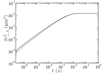
Figure 3: Comparison of different approximations of the MSD $\delta r_{\perp,\Lambda}^{2}$ of a WLC of length $\Lambda=1\,\upmu\mbox{m}$ ($\ell_{p}=1\,\upmu\mbox{m}$) with hydrodynamic interactions: numerical evaluation of eq. (70) (—), simple analytical approximation eq.  (62) with time dependent friction constant $\zeta_{\perp}(t)$ ($-\,-$) and improved approximation eq. (LABEL:msdlogtot) ($\dots$).

If the $z$-integration in eq. (29) is carried out for $s=s^{\prime}$, the dynamic MSD $\delta r_{\perp}^{2}(t)\equiv\overline{\delta r_{\perp}^{2}(s,s,t)}$ of a free polymer of infinite length is recovered:

$$\delta r_{\perp}^{2}(t)=\frac{\ell_{\perp}^{3}(t)}{\pi\ell_{p}}\frac{\Gamma(1/4)}{3}=\frac{\Gamma(1/4)}{3\pi q^{2}}(\Gamma_{q}^{(s)}t)^{3/4}.$$ (31)

The full mean square displacement consists of a static and the dynamic part,

$$\begin{split}\Delta r_{\perp}^{2}(s,s^{\prime},t)&\equiv\langle[\mathbf{r}_{\perp}(s,t)-\mathbf{r}_{\perp}(s^{\prime},0)]^{2}\rangle\\ &=\langle[\mathbf{r}_{\perp}(s,0)-\mathbf{r}_{\perp}(s^{\prime},0)]^{2}\rangle+\delta r_{\perp}^{2}(s,s^{\prime},t)\end{split}$$ (32)

It is easy to see by a Taylor expansion, that in the bulk of the polymer the static MSD between two different points on the contour is to leading order quadratic in the contour length, $\Delta r_{\perp}^{2}(s,s^{\prime},0)\simeq\epsilon(s-s^{\prime})^{2}/2$. More precisely, a systematic calculation for hinged ends gives glaser:unpub2

$$\Delta r_{\perp}^{2}(s,s^{\prime})=\frac{1}{6}\ell_{p}^{-1}L^{3}\Big{\{}(\tilde{s}^{\prime}-\tilde{s})^{2}\big{\{}1+\\ 4\big{[}(1/2-\tilde{s})^{2}+(1/2-\tilde{s})(1/2-\tilde{s}^{\prime})+(1/2-\tilde{s}^{\prime})^{2}\big{]}\big{\}}\\ -2|\tilde{s}^{\prime}-\tilde{s}|^{3}\Big{\}}\quad(\tilde{s}\equiv s/L,\,\tilde{s}^{\prime}\equiv s^{\prime}/L).$$ (33)

The terms in the middle as well as the last one can be neglected in the bulk of the polymer, where $|s-L/2|\ll L/2$. For long times, only the dynamic part of the MSD evaluated at $s=s^{\prime}$ contributes to the deacy of the dynamic structure factor, resulting in the incoherent dynamic structure factor Kroy2000 .

In the remainder of this section, we discuss extensions of the theory for isolated filaments that address the effects of the surrounding solution. For completeness, we first briefly summarize the idea behind and the most important prediction of the standard tube model, before we describe the alternative GWLC model, which compares more favorably to a large body of experimental data.

3.2 The tube model

Quasi-static quantities, such as the plateau modulus of a solution of semiflexible polymers are satisfactorily explained by the tube model, which assumes that the effect of the surrounding network may effectively be represented by a tube-like cage, see e.g. Isambert1996 ; Morse2001 ; Kroy2006 ; Hinsch2007 . The tube properties are characterized by the entanglement length $L_{e}$ (the arc length over which the bending energy equals the confinement energy) or equivalently by the tube diameter $d$. Both quantities are related by the basic roughness relation $d^{2}\simeq L_{e}^{3}/\ell_{p}$ of the WLC, which also implies that the transverse mean-square deflections from a clamped end grow like the third power of the wavelength.

In the simplest static version of a harmonic tube potential, which is added to the Hamiltonian, the relaxation of a confined polymer is exponentially suppressed for times longer than the entanglement time $\tau_{e}$ associated with a mode of wavelength $k^{-1}\simeq L_{e}$ Janmey1994 . The saturation of the MSD and the dynamic structure factor to their plateau values is however too quick if compared to experimental observations. This is improved by an extension of the tube model that includes dynamic fluctuations of the tube arising from an over-damped homogeneous elastic background material Kroy2000 , which yields

$$\delta r_{\perp}^{2}(t)=\langle\mathbf{r}^{2}\rangle\left[1-\frac{\sqrt{\pi}}{2}\frac{\mbox{erf}(\sqrt{\omega_{\star}t})}{\sqrt{\omega_{\star}t}}\right]+\\ \langle\mathbf{r}_{\perp}^{2}\rangle\left[1-\frac{3}{4}(\omega_{\star}t)^{3/4}\Gamma(-3/4,\omega_{\star}t)\right]\;.$$ (34)

Here, the prefactors $\langle\mathbf{r}^{2}\rangle$ and $\langle\mathbf{r}_{\perp}^{2}\rangle$ are the mean squared amplitudes of the effective medium and of the polymer, respectively, $\omega_{\star}$ is approximately (but not strictly) identical to the inverse of the entanglement time $\tau_{e}$. Theoretically, the static MSD, to which the dynamic MSD saturates algebraically (like $t^{-1/2}$), is connected to the crossover frequency $\omega_{\star}$ via

$$\langle\mathbf{r}_{\perp}^{2}\rangle=\frac{4}{3\pi}\left(\frac{k_{B}T\omega_{\star}^{-1}}{\zeta_{\perp}\ell_{p}^{1/3}}\right)^{3/4}\;.$$ (35)

While this model seems to agree reasonably well with experimental data Mason2000 ; Liu2006 ; Vincent2007 if the amplitudes and the crossover frequency are treated as free fit parameters, it cannot account for the ‘slanted plateaus’ generally observed, which correspond to a very slow terminal relaxation of the MSD.

3.3 The basic idea of the glassy wormlike chain (GWLC)

It is only very recently that high-precision DLS experiments unambiguously demonstrated a slow logarithmic terminal relaxation instead of a plateau in the dynamic structure factor of actin solutions at low temperatures Semmrich2007 . This has been interpreted as a signature of a system near its glass transition, which only slowly relaxes into equilibrium. An interpretation of the logarithmic tails in the framework of the established mode coupling theory for glasses Gotze1991 , as suggested by recent simulation studies of flexible polymer blends Moreno2006 , would require an improbable fine tuning of parameters into the neighborhood of a higher-order mode coupling singularity. It therefore seems at variance with the generic nature of the slow relaxation in actin solutions, which is found to extend over more than three decades in time Semmrich2007 and observed for a wide range of concentrations. For the same reasons, and additionally for the lack of any observations of a percolation structure in actin solutions, an interpretation in terms of a percolation critical point seems unnatural to us.

In contrast to models attributing the stretching of the relaxation spectrum to a critical point, the GWLC Kroy2007 suggests a very intuitive origin of the slow-down in a rough free energy landscape. The basic assumption of the model in its simplest form is that short wavelength modes with a (half) wavelength $\lambda_{n}\equiv\pi/k_{n}<\Lambda$ can relax freely, while for the relaxation of a mode $n$ with $\lambda_{n}>\Lambda$ a certain number $N_{n}$ of energy barriers of height ${\cal E}k_{B}T$ have to be overcome. This prescription is in the spirit of the generic trap models recently favored by many experimental investigators of cell mechanics Fabry2001 ; Lenormand2006 , but it puts them on a more concrete basis. Physically the parameter ${\cal E}$ is thought to arise primarily from direct adhesive polymer interactions Kroy2007 . But in the same vein steric caging and entanglement effects may be cast into the language of free energy barriers by a free volume argument. Assigning an Arrhenius factor for each free energy barrier, the above prescription gives rise to an anomalous stretching of the WLC relaxation spectrum that manifests itself in anomalously slow (logarithmic) decay of single-polymer conformational correlations at long times. Implementing the corresponding prescriptions in eq. (58) for the dynamic MSD of a WLC, one obtains the predictions of the GWLC for the late time dynamics. Fig. 4 illustrates the effect of different types of interactions of the test chain with its surrounding medium on the dynamic MSD, and compare them to the predictions of the classical tube model. A similar comparison for the structure factor is presented further below. We remark that experimental evidence of logarithmic relaxation (or near-constant loss in the susceptibility spectra) observed for synthetic polymer melts Sokolov2001 could be indicative of a mechanism akin to that proposed for the GWLC in these systems. This observation has recently prompted the introduction of the ‘glassy Rouse chain’ Glaser2008 .

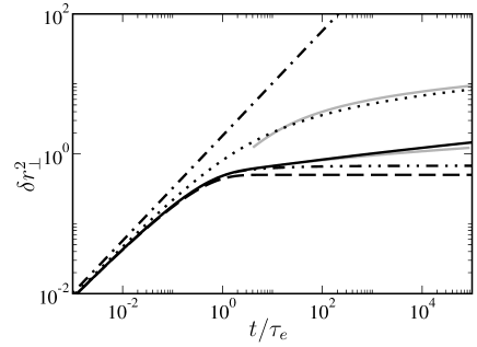
Figure 4: MSD of a free polymer ($-\cdot-$), of a polymer in an overdamped elastic background (– $\cdot\cdot$) with $\langle\mathbf{r}^{2}\rangle=0.35\,\langle\mathbf{r}_{\perp}^{2}\rangle$, GWLC with purely steric interactions ($\cdots$), and a GWLC with purely sticky interactions according to $\Lambda=L_{e}$, ${\cal E}=\infty$ ($--$) (equivalent to a static tube) and ${\cal E}=25$ (—), all with $\delta r_{\perp,L_{e}}^{2}(\infty)=\langle\mathbf{r}_{\perp}^{2}\rangle/3=4L_{e}^{3}/3\ell_{p}\pi^{4}=0.5$. The approximate analytical expressions eqs. (15), (62) and the asymptotic result eqs. (12), (62) (for $t>\tau_{e}e^{-{\cal F}}\!/{\cal F}$ with $\Lambda\rightarrow L_{e}$) are shown in gray.

3.4 Direct sticky interactions in the GWLC

In the simplest version, the GWLC behavior arises from very short-ranged (sticky) interactions of crossing polymers, as they might arise from hydrogen bonds or hydrophobic patches on a biopolymer’s backbone, or dispersion forces that are cut off at short distances. If such interactions are imperfectly screened by electrostatic repulsions, the resulting pair interaction potential will feature an energy barrier, which is denoted by ${\cal E}k_{B}T$ Kroy2007 . While such interactions may under some conditions induce phase separation, we concentrate on conditions of moderate attractions, where they have no thermodynamic but merely a kinetic effect via the barrier. In this case, the strategy of keeping the equilibrium mode amplitudes $\langle\mathbf{a}_{n}^{2}\rangle$ of the WLC unchanged while modifying its relaxation spectrum should be adequate. (In fact, the question how the equilibrium amplitudes are renormalized by the presence of a disordered background poses a formidable theoretical challenge, but the following analysis suggests that it might not be the dominant effect for the dynamics.)

Whenever such sticky interactions are the dominant effect, the relaxation spectrum of the bare WLC is modified according to

$$\tilde{\tau}_{n}=\begin{cases}\tau_{n}&n>n_{\Lambda}=L/\Lambda\\ \tau_{n}\exp(N_{n}{\cal E})&n<n_{\Lambda}\\ \end{cases}$$ (36)

with

$$N_{n}\equiv(\lambda_{n}/\Lambda-1)\;.$$ (37)

Here, $n_{\Lambda}$ denotes the interaction wave number, so that only two new parameters are introduced: the stretching parameter or barrier height ${\cal E}$ and the interaction length $\Lambda$, which has the direct physical interpretation as a typical contour distance between sticky contacts. For example, if the polymer contour as a whole is highly sticky, $\Lambda$ will be identical to the entanglement length $L_{e}$. When the stickiness is only induced at certain places along the backbone, e.g. if it is due to an incomplete coverage of the backbone with some molecular crosslinker, $\Lambda$ may be substantially larger than $L_{e}$. The same role is actually played by the strength of the attraction in the sticky case, where it determines the equilibrium ratio of bound to unbound entanglement points and thus $\Lambda/L_{e}$ via a Boltzmann factor. In particular in cases where ${\cal E}\lesssim 1$ and/or $\Lambda\gg L_{e}$ it becomes important to also consider the effect of steric interactions between adjacent polymers, known as cageing or entanglement, which is the subject of the following paragraph.

3.5 Cageing and entanglements in the GWLC

The GWLC model as introduced above is applicable to systems dominated by adhesive interactions. Additional contributions to the stretching of the relaxation spectrum arise however from steric interactions of the chain with its surroundings. Our basic assumption is that for each wavelength there are several substantially different conformations of similar free energy available. In order to relax the caged long wavelength modes, the surrounding matrix then has to be temporarily pushed out of the way to create enough free volume for the conformational change, a process that can again be described by an escape over a free energy barrier. More precisely, a wavelength dependent entanglement volume $V_{\lambda}$ may be defined as the free volume needed by a mode of (half) wavelength $\lambda$ to relax, which depends on the magnitude of the transverse excursions. These may be inferred from the following simple argument: With the help of eq. (22) the MSD of a monomer after relaxation of a mode of wavelength $\lambda=L/n$ is calculated as

$$\delta r_{\perp,\lambda}^{2}=\frac{2}{L}\sum\limits_{n=L/\lambda}^{\infty}\langle\mathbf{a}_{n}^{2}\rangle\approx\frac{4L^{3}}{\pi^{4}\ell_{p}}\int\limits_{L/\lambda}^{\infty}\frac{\mbox{d}n}{n^{4}}\,\simeq\lambda^{3}/\ell_{p}$$ (38)

(where the spatial averaging has already been carried out). Accordingly, we have $V_{\lambda}=\lambda\delta r_{\perp,\lambda}^{2}\propto\lambda^{4}$. The free energy barrier, that a mode of (half) wavelength $\lambda$ has to overcome to relax in presence of a background polymer solution of entanglement length $L_{e}$ is then estimated as $k_{B}T{\cal F}\lambda^{4}/L_{e}^{4}$. Moreover, it is assumed that modes with a transverse MSD smaller than $\delta r^{2}_{\perp,L_{e}}$ can relax freely. Similar to the above case with adhesive interactions, this leads to an additional stretching of the relaxation spectrum, where the relaxation times of modes of wavelength $\lambda_{n}>L_{e}$ are slowed down according to

$$\tilde{\tau}_{n}=\begin{cases}\tau_{n}&n>n_{e}=L/L_{e}\\ \tau_{n}\exp(N_{n}^{\prime}{\cal F})&n<n_{e}\\ \end{cases}$$ (39)

with

$$N_{n}^{\prime}\equiv(\lambda^{4}_{n}/L_{e}^{4}-1).$$ (40)

The dimensionless free energy barrier height ${\cal F}$ is generally expected to have a small numerical value, as can be seen from the following argument. The interaction free energy of a rigid polymer segment with hard core interactions is estimated as $cvk_{B}T/2$, where $c$ is the concentration of collision points and $v$ is the excluded volume of the segments. Here we consider semiflexible polymers of length $L_{e}$ with purely hard core direct interactions that are represented as soft cylinders interacting via an effective potential $V(r)$ on a coarse-grained level. Comparing their mutual repulsion to a hard core interaction, we estimate ${\cal F}\simeq 2B_{2}/v$, where $B_{2}$ is the second virial coefficient of the solution of soft cylinders. The effective interaction potential between the cylinders, is due to a kind of Helfrich repulsion Helfrich1985 ; Daniels2004 . Consider two WLCs of length $L_{e}$ that approach each other at orthogonal orientations. If the two axes through the polymer endpoints are held at a fixed distance $r$ from each other, their effective interaction potential $V(r)$ is found to be Teeffelen ; Morse2001

$$V(r)=-k_{B}T\log\left[\mbox{erfc}(-2\sqrt{3}r/d)/2\right]\;,\qquad d=\sqrt{L_{e}^{3}/\ell_{p}},$$ (41)

From this, the second virial coefficient is calculated as an integral over the Mayer $f$-function,

$$B_{2}=-\frac{1}{2}\int\mbox{d}\,\mathbf{r}\int\frac{\mbox{d}\Omega}{4\pi}\,\int\frac{\mbox{d}\Omega}{4\pi}^{\prime}\,\{\exp[-\beta V(\mathbf{r},\Omega,\Omega^{\prime})]-1\},$$ (42)

where $\mathbf{r}$ denotes relative separation between the two axes and $\Omega,\Omega^{\prime}$ denote their orientations. The implicit assumption is made that the potential of the two polymers crossing at an arbitrary angle is still of the form for orthogonally crossing polymers. The integral is split into a surface integral over a parallelogram (with edges of the tube length $L_{e}$) in the plane spanned by two unit vectors in the direction of $\Omega,\Omega^{\prime}$ (the excluded area) and an integral over the distance of the cylinders in a direction transverse to this plane, and it is assumed that the interaction potential only depends on this distance. One arrives at $B_{2}=L_{e}^{2}d\sqrt{\pi}/8\sqrt{3}$, and using $v=\pi L_{e}^{2}d/2$ for the excluded volume of hard cylinders of diameter $d$ and length $L_{e}$ Onsager1949 , we get:

$${\cal F}\approx\frac{1}{\sqrt{\pi}2\sqrt{3}}\approx 0.2.$$ (43)

For the strength of the steric interactions in Figs. 4-5, this value of ${\cal F}$ is used. It should be noted that ${\cal F}$ must in principle be recalculated if attractive interactions are present, in which case its absolute value can be substantially smaller. For strongly attractive interactions, ${\cal F}$ may turn negative, indicating that the free volume approach breaks down. The value for ${\cal F}$ obtained in eq. (43) should thus be understood as a rough estimate of an upper limit for purely steric interactions, while in the case $\Lambda\simeq L_{e}$ of strong stickiness, ${\cal F}\rightarrow 0$.

4 The dynamic structure factor

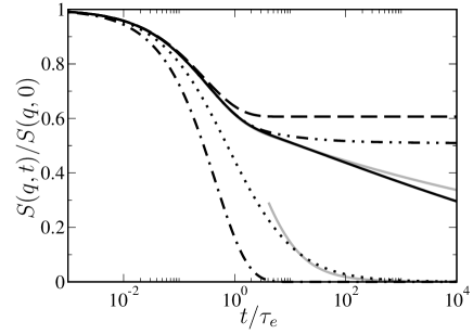
Figure 5: Dynamic structure factor of a free polymer ($-\cdot-$), of a polymer in an overdamped elastic background (– $\cdot\cdot$) with $\langle\mathbf{r}^{2}\rangle=0.35\,\langle\mathbf{r}_{\perp}^{2}\rangle$, of a GWLC with purely steric interactions ($\cdots$), and a GWLC with purely sticky interactions according to $\Lambda=L_{e}$ and ${\cal E}=\infty$ ($--$) (equivalent to a static tube) and ${\cal E}=25$ (—), all with $\delta r_{\perp,L_{e}}^{2}(\infty)=\langle\mathbf{r}_{\perp}^{2}\rangle/3=4L_{e}^{3}/3\ell_{p}\pi^{4}=0.5$. The dynamic structure factors obtained from the approximate analytical expressions eqs. (3), (15), (62) and the asymptotic result eqs. (3), (12), (62) (for $t>\tau_{e}e^{-{\cal F}}\!/{\cal F}$ with $\Lambda\rightarrow L_{e}$) are shown in gray.

4.1 Initial decay ($t\ll\tau_{q}^{\perp}$)

In this section we discuss the initial decay regime of the dynamic structure factor of (isolated) semiflexible filaments. Our calculation will be different from that in refs. Kroy1997 ; Liverpool2001 ; Nyrkova2007 , which was performed in mode space or Fourier space respectively, whereas our approach employs a real space representation.

To perform the thermal average in the dynamic structure factor eq. (1), the assumption that $\mathbf{r}_{\perp}$ is a Gaussian distributed variable is employed, valid for situations where the scattering can be traced back to single polymers which are described by eq. (21), i.e., whenever the scattering wavelength is smaller than the mesh size ($q^{-1}\ll\xi$). A quantitative evaluation of the derived results should thus focus on the largest measurable values of $q$. Neglecting longitudinal fluctuations, we get

$$S(q,t)=\frac{1}{Ld}\int\mbox{d}s\int\mbox{d}s^{\prime}\langle\exp[-q_{\perp}^{2}\Delta r_{\perp}^{2}(s,s^{\prime},t)/4\\ +iq_{\|}(s-s^{\prime})]\rangle_{O},$$ (44)

where $q_{\|}=q\cos(\theta)$ and $q_{\perp}^{2}=q^{2}\sin^{2}(\theta)$.

$$\langle\dots\rangle_{O}\equiv(1/2)\int\limits_{0}^{\pi}\mbox{d}\theta\,\sin(\theta)$$ (45)

denotes an average over orientations of the polymer. Taking this average, we get in the limit $q^{2}\Delta r_{\perp}^{2}(t)\ll 1$ ($t\rightarrow 0$)

$$S(q,t)\approx\frac{1}{2Ld}\int\mbox{d}s\,\mbox{d}s^{\prime}\,\int\limits_{-1}^{1}\mbox{d}x\,[1-q^{2}(1-x^{2})\Delta r_{\perp}^{2}(s,s^{\prime},t)/4\\ +\dots]\exp[iqx(s-s^{\prime})].$$ (46)

For $t=0$ and to zeroth order in $\epsilon$, the expression for the static structure factor is obtained:

$$S(q,0)\approx\frac{1}{2Ld}\int\mbox{d}s\,\mbox{d}s^{\prime}\,\int\limits_{-1}^{1}\mbox{d}x\,\exp[iqx(s-s^{\prime})]=\frac{\pi}{qd}.$$ (47)

The initial decay rate is defined as

$$\Gamma_{q}^{(0)}\equiv-\lim_{t\rightarrow 0}\frac{\mbox{d}}{\mbox{d}t}\log(S(q,t)).$$ (48)

We therefore need to calculate $\partial_{t}\Delta r_{\perp}^{2}(s,s^{\prime},t)$. We have

$$\lim_{t\rightarrow 0}\partial_{t}\Delta r_{\perp}^{2}(s,s^{\prime},t)=-2\lim_{t\rightarrow 0}\langle\mathbf{r}_{\perp}(s^{\prime},0)\partial_{t}\mathbf{r}_{\perp}(s,t)\rangle\\ +2\lim_{t\rightarrow 0}\langle\mathbf{r}_{\perp}(s,t)\partial_{t}\mathbf{r}_{\perp}(s,t)\rangle.$$ (49)

The last term in eq. (49) is actually a time derivative of an equilibrium correlation function and vanishes consequently. We replace the first time derivative using the equation of motion, eq. (21), and thus get an integral over an equilibrium correlation function for the transverse coordinates:

$$\lim_{t\rightarrow 0}\partial_{t}\Delta r_{\perp}^{2}(s,s^{\prime},t)\\ =2\kappa\lim_{t\rightarrow 0}\int_{0}^{L}\mbox{d}\tilde{s}\,h(s-\tilde{s})\langle\mathbf{r}_{\perp}^{\prime\prime\prime\prime}(\tilde{s},t)\mathbf{r}_{\perp}(s^{\prime},0)\rangle$$ (50)

The last correlator is obtained via the equipartition theorem, which yields

$$\langle\mathbf{r}_{\perp}^{\prime\prime\prime\prime}(\tilde{s})\mathbf{r}_{\perp}(s^{\prime})\rangle=2\ell_{p}^{-1}\delta(\tilde{s}-s^{\prime}),$$ (51)

taking into account two transverse directions. Combining eqs. (46), (50) and (51) we get

$$\lim_{t\rightarrow 0}\partial_{t}S(q,t)=-\frac{k_{B}Tq^{2}}{2Ld}\int\mbox{d}s\,\mbox{d}s^{\prime}\,\int\limits_{-1}^{1}\mbox{d}x\,h(s-s^{\prime})(1-x^{2})\\ \times\cos(qx(s-s^{\prime})).$$ (52)

With the help of the general identity

$$\int\limits_{0}^{L}\mbox{d}s\,\int\limits_{0}^{L}\mbox{d}s^{\prime}\,f(s-s^{\prime})=\int\limits_{-L}^{L}\mbox{d}s\,f(s)(L-|s|)$$ (53)

and eq. (47) we find the general expression for the initial decay rate

$$\Gamma_{q}^{(0)} =\lim_{t\rightarrow 0}\frac{\partial_{t}S(q,t)}{S(q,0)}$$ (54)

$$=\frac{k_{B}Tq^{3}}{2\pi L}\int\limits_{-L}^{L}\mbox{d}s\,\int\limits_{-1}^{1}\mbox{d}x\,(L-|s|)h(s)(1-x^{2})\cos(qxs).$$ (55)

Using the mobility function, eq. (20), an evaluation of eq. (55) for $d\ll q^{-1}\ll L$, an assumption usually fulfilled in light scattering experiments on biopolymers, gives

$$\Gamma_{q,RP}^{(0)}=\frac{k_{B}Tq^{3}}{6\pi^{2}\eta}[C-\log(qd)].$$ (56)

(terms of order $(qd)^{2}$ and higher have been discarded and the limit $L\rightarrow\infty$ has been taken.) The constant is $C=4/3+17/12-\gamma_{E}=2.17$, where $\gamma_{E}$ is Euler’s constant. This value differs from the previously reported value of $C=5/6$ Kroy1997 . We attribute this to our improved treatment of the hydrodynamic interactions. However, it also shows that the exact value sensitively depends on the details of the hydrodynamic model, which has to be taken into account for the determination of the hydrodynamic backbone diameter from measurements of the initial decay rate. This is also acknowledged in Nyrkova2007 . While our result confirms the previous results found in Kroy1997 ; Nyrkova2007 , Liverpool and Maggs Liverpool2001 obtained a qualitatively different result, where an additional logarithmic factor $S(q,t)/S(q,0)-1\simeq t\log(t)$ appears in the short time behavior of the dynamic structure factor, diverging in the limit $t\rightarrow 0$. This results from their too inaccurate treatment of the spherical Bessel functions occurring in the discussion in mode space.

We remark that if one chooses the simpler Oseen expression for the mobility function, our result for the initial decay rate due to transverse displacements, eq. (55), reduces (after carrying out the integration over $x$ and in the limit $L\rightarrow\infty$) to a result quoted in refs. Doi1988 ; Nyrkova2007 , which is derived from the Smoluchowski equation by projecting out longitudinal degrees of freedom from the mobility tensor, as proposed also in Kroy1997 . This amounts to evaluating eq. (21) of Nyrkova2007 with their scaling function replaced with ${\cal H}(x)=(1+\mbox{d}^{2}/\mbox{d}x^{2})\sin(x)/x$. An advantage of our approach over the calculation via the Smoluchowski equation lies in the fact that the Rotne-Prager corrections can easily be implemented in the mobility function. Table 1 compares the different predictions for the constant $C$ in eq. (56).

4.2 Logarithmic tails ($t\gg\tau_{e}$)

Since the dynamic structure factor at long delay times is of the (incoherent) form

$$S(q,t)\sim S(q,0)\exp[-q^{2}\delta r_{\perp}^{2}(t)/4]\;,$$ (57)

its late time behavior is trivially obtained from the dynamic MSD. Upon exponentiating, Fig. 4 is translated into Fig. 5. Interestingly, the somewhat limited logarithmic intermediate asymptotics visible in the MSD in the strongly sticky limit ${\cal E}\gg 1$ is thereby extended to much longer times, so that a logarithmic intermediate decay seems to constitute a quite robust feature of the dynamic structure factor of semidilute solutions of sticky semiflexible polymers (cf. Fig. 2). The remainder of this paragraph is therefore dedicated to a closer examination of the analytical properties of this intermediate asymptotics. For simplicity, we set ${\cal F}=0$ for the following discussion (the case ${\cal F}>0$ is discussed in appendix B).

We start from the dynamic MSD of a WLC and introduce the stretched relaxation times $\tilde{\tau}_{n}$ eq. (36). For convenience, we quote the general expression for the MSD by converting eq. (28) to an integral, after taking the limit $L,n_{\Lambda}\rightarrow\infty$ with $\Lambda=\mbox{const.}$,

$$\delta r_{\perp}^{2}(t)=\overline{\delta r_{\perp}^{2}(s,s,t)}=\frac{4L^{3}}{\pi^{4}\ell_{p}}\int\limits_{0}^{\infty}\frac{\mbox{d}n}{n^{4}}\,[1-\exp(-t/\tilde{\tau}_{n})].$$ (58)

We perform a change of variables and the dynamic MSD is written as

$$\delta r_{\perp}^{2}(t)=\delta r_{\perp,\Lambda}^{2}(t)+\delta r_{\perp}^{2,G}(t),$$ (59)

where

$$\delta r_{\perp,\Lambda}^{2}(t)=\frac{4\Lambda^{3}}{\ell_{p}\pi^{4}}\int\limits_{1}^{\infty}\frac{\mbox{d}n}{n^{4}}\,\{1-\exp[-(t/\tau_{\Lambda})n^{4}]\},$$ (60)

with $\tau_{\Lambda}=(\zeta_{\perp}/\kappa)(\Lambda^{4}/\pi^{4})$ (note that we assume the simplified treatment of hydrodynamic interactions here, for an improved discussion of eq. (60) see appendix A), and

$$\delta r_{\perp}^{2,G}(t)=\frac{4\Lambda^{3}}{\ell_{p}\pi^{4}}\\ \times\int\limits_{0}^{1}\frac{\mbox{d}n}{n^{4}}\,\{1-\exp\{-(t/\tau_{\Lambda})n^{4}\exp[-{\cal E}(1/n-1)]\}\}.$$ (61)

For the slow modes of eq. (61), substituting $\overline{\ell}_{\perp}(t)=\Lambda/\pi$ in the friction constant $\zeta_{\perp}(t)$ is sufficient. The first integral can be expressed in terms of an incomplete Gamma function,

$$\delta r_{\perp,\Lambda}^{2}(t)=\frac{4\Lambda^{3}}{3\ell_{p}\pi^{4}}\left\{1-b(t/\tau_{\Lambda})^{b}\Gamma[-b,(t/\tau_{\Lambda})]\right\},$$ (62)

where $b=3/4$. (This term is of the same form as the right term in eq. (34).) The integral saturates in the limit of long times,

$$\delta r_{\perp,\Lambda}^{2}(\infty)=4\Lambda^{3}/3\ell_{p}\pi^{4}.$$ (63)

The second integral is not immediately solvable analytically. We approximate it within a certain range of parameters. Writing

$$\tilde{n}=\tilde{t}^{1/4}\exp[-({\cal E}/4)(1/n-1)]n,$$ (64)

with the rescaled time $\tilde{t}=t/\tau_{\Lambda}$, we approximatively solve the implicit equation for $n$ and get

$$n \approx\frac{1}{1-(4/{\cal E})\log(\tilde{n}/n_{0}\tilde{t}^{1/4})}$$ (65)

$$\mbox{d}n \approx\frac{4}{{\cal E}}\frac{\mbox{d}\tilde{n}}{[1-(4/{\cal E})\log(\tilde{n}/n_{0}\tilde{t}^{1/4})]^{2}\tilde{n}}.$$ (66)

It is possible to numerically determine the fixed mode number $n_{0}$. This substitution is valid as long as the logarithmic term in the denominator of eqs. (65), (66) is not dominant, i.e.  for ${\cal E}\gg 1$. The remaining integral then reads:

$$\begin{split}\delta r_{\perp}^{2,G}(t)&\approx\frac{4\Lambda^{3}}{\ell_{p}\pi^{4}}\frac{4}{{\cal E}}\int\limits_{0}^{\tilde{t}^{1/4}}\frac{\mbox{d}\tilde{n}}{\tilde{n}}\,[1-\exp(-\tilde{n}^{4})]\\ &\quad\qquad\qquad\qquad\times\left[1-\frac{4}{{\cal E}}\log(\tilde{n}/n_{0}\tilde{t}^{1/4})\right]^{2}\\ &\approx\frac{4\Lambda^{3}}{\ell_{p}\pi^{4}}(A-B).\end{split}$$ (67)

These two integrals can be performed,

$$A=\frac{4}{{\cal E}}\int\limits_{0}^{\tilde{t}^{1/4}}\frac{\mbox{d}\tilde{n}}{\tilde{n}}\,[1-\exp(-\tilde{n}^{4})]\\ =\frac{1}{{\cal E}}[\gamma_{E}-\mbox{Ei}(-\tilde{t})+\log(\tilde{t})]$$ (68)

and

$$\begin{split}B&=\frac{32}{{\cal E}^{2}}\int\limits_{0}^{\tilde{t}^{1/4}}\frac{\mbox{d}\tilde{n}}{\tilde{n}}\,[1-\exp(-\tilde{n}^{4})]\log(\tilde{n}/n_{0}\tilde{t}^{1/4})\\ &\approx\frac{8}{{\cal E}^{2}}[-1/4-\log(n_{0})]\tilde{t}+{\cal O}(\tilde{t})^{2}\qquad(\tilde{t}\ll 1).\end{split}$$ (69)

In the limit $\tilde{t}/{\cal E}\ll 1$ we can neglect the contribution of $B$ (which for long times is ultimately approximated by a logarithmic term in $t$ resulting in corresponding power-law-decay in the dynamic structure factor) against $A$ and the final result, valid for short and intermediate times, is provided by eq. (15). Combining eq. (11), and (15), observing that $\mbox{Ei}(-\tilde{t})\rightarrow 0\,(\tilde{t}\rightarrow\infty)$, we arrive at eq. (16). A comparison of the result eq. (15) to the numerically evaluated expression eq. (61) is shown in Figs. 4, 5.

As the direct numerical evaluation in Figs. 2, 5 shows, the logarithmic tail of the structure factor for large ${\cal E}$ extends well beyond the indicated time regime $t\ll{\cal E}\tau_{\Lambda}$. It follows from eq. (16) that the prefactor of the logarithm (the slope of the logarithmic tail in a semilogarithmic plot) is inversely proportional to the energy barrier height ${\cal E}$, which is therefore directly monitored by the slope of the tail of the structure factor plotted against $\ln t$. Both $\Lambda$ and ${\cal E}$ can be accurately determined from a fit of eq. (3) to experimental data with the $\delta r_{\perp}^{2}(t)$ given by the full model eqs. (59), (62), (15).

5 Conclusions and outlook

We have presented a thorough theoretical discussion of the dynamic structure factor of a stiff polymer in a (sticky) solution. We claim that our predictions, though in qualitative agreement with previous results, are quantitatively superior and provide the missing link to a reliable quantitative analysis of microscopic mechanical parameters of polymers (backbone diameter and persistence length) via dynamic scattering measurements. Even more important seem the prospects of applying quasi-elastic scattering as a matchless non-invasive microrheological technique to explore with high accuracy the so far poorly understood parameter dependencies of the GWLC stretching parameter ${\cal E}$. This represents in our opinion one of the most promising pathways towards a microscopic modeling of the mechanical properties of biopolymer networks and living cells. A particularly rewarding application might be the search for an apparently scale dependent persistence length of biopolymers Heussinger2007a , which might arise from the fact that these polymers have a fibrous substructure requiring a GWLC (rather than a WLC) description already on the single polymer level.

Appendix A Analytical approximation to hydrodynamic interactions

In this section we will derive an analytical approximation for the mode integral of the MSD of the free GWLC modes, eq. (60), which is also the part of the MSD which corresponds to a static tube. We rewrite the integral with the help of eq. (24):

$$\delta r_{\perp,\Lambda}^{2}(t)=\frac{4\Lambda^{3}}{\ell_{p}\pi^{4}}\int\limits_{1}^{n_{0}}\frac{\mbox{d}n}{n^{4}}\,\left\{1-\exp[-(t/\overline{\tau}_{\Lambda})n^{4}\log(n_{0}/n)]\right\},$$ (70)

where $n_{0}\equiv\Lambda\exp(C^{\prime})/\pi d$ is an upper mode cut-off corresponding to the finite backbone diameter and $\overline{\tau}_{\Lambda}\equiv(4\pi\eta/\kappa)(\Lambda/\pi)^{4}$ is the approximate relaxation time of a mode of wavelength $\Lambda$. We begin with a substitution of variables, $z^{4}\equiv n^{4}\log(n_{0}/n)$. The lower bound of the integral is then $z_{0}=\log^{1/4}n_{0}$. With $\alpha\equiv 4z^{4}/n^{4}$, $n(z)$ is determined if $\alpha$ is a solution to the equation:

$$\alpha\exp(-\alpha)=4\frac{z^{4}}{n_{0}^{4}}.$$ (71)

Two solutions for $-\alpha$ exist: the two real branches of the Lambert $W$-function. In our case, the dominant contribution to the integral comes from the mode numbers for which $n\ll n_{0}$, this corresponds to $z>n$ or $\alpha\gg 1$. The relevant solution is therefore given by $\alpha=-W_{-1}(-4z^{4}/n_{0}^{4})$. This defines the upper bound of the integral as $z_{1}=(4e)^{-1/4}n_{0}$. We then have $W_{-1}(-4z^{4}/n_{0}^{4})=-4z^{4}/n^{4}$, and, using the derivative of the Lambert $W$ function, $W_{-1}^{\prime}(x)=W_{-1}(x)/\{x[1+W_{-1}(x)]\}$,

$$\mbox{d}n=\sqrt[4]{\frac{4}{\alpha}}\left(1-\frac{1}{1-\alpha}\right)\mbox{d}z.$$ (72)

The Lambert $W$ function may be asymptotically approximated by $W_{-1}(-x)=\gamma+\log(x)$ for $x\ll 1$ with $|\gamma|\ll|\log(x)|$ Corless1996 . Here we choose $\gamma=W_{-1}(-x_{0})-\log(x_{0})$, i.e., we expand $W_{-1}(-x)-\log(x)$ to $0th$ order around $x_{0}\equiv-4z_{0}^{4}/n_{0}^{4}$ (This means, that for very high mode numbers or very short times the approximation breaks down.) For the purpose of numerical evaluation, analytical approximations to $W_{-1}$ may be used Barry2000 . Hence we have the following expression for the integral eq. (70):

$$\delta r_{\perp,\Lambda}^{2}(t)\approx\frac{4\Lambda^{3}}{\ell_{p}\pi^{4}}4^{-3/4}\int\limits_{z_{0}}^{z_{1}}\mbox{d}z\,\alpha^{3/4}(z)\left(1-\frac{1}{1-\alpha}\right)\\ \frac{1-\exp[-(t/\overline{\tau}_{\Lambda})]}{z^{4}}.$$ (73)

Consider the first factor in the integrand. It is

$$\begin{split}\alpha^{3/4}(z)&=\left[-W_{-1}\left(-\frac{4z^{4}}{n_{0}^{4}}\right)\right]^{3/4}\\ &\approx\left[-\gamma(z_{0})-\log\left(\frac{4z^{4}}{n_{0}^{4}}\right)\right]^{3/4}\quad(z\ll n_{0})\\ &\approx\left[-\log\left(\frac{4z^{4}}{n_{0}^{4}}\right)\right]^{3/4}\\ &\qquad\qquad\qquad\left[1+\frac{3}{4}\frac{\gamma(z_{0})}{\log(4z^{4}/n_{0}^{4})}\right].\end{split}$$ (74)

We approximate the first factor in eq. (74) for $z\ll n_{0}$ as

$$\left[-\log(4z^{4}/n_{0}^{4})\right]^{3/4}\approx 4^{3/4}\log^{3/4}n_{0}\left[1-\frac{3}{4}\frac{\log(\sqrt{2}z)}{\log n_{0}}\right],$$ (75)

and the $1/\log(\dots)$ term in the second factor as

$$\begin{split}\frac{1}{\log(4z^{4}/n_{0}^{4})}&\approx\frac{-1}{4\log n_{0}\left[1-\frac{\log(\sqrt{2}z)}{\log n_{0}}\right]}\\ &\approx\frac{-1}{4\log(n_{0})}\left[1+\frac{\log(\sqrt{2}z)}{\log n_{0}}\right].\end{split}$$ (76)

Taken together, one finds, after grouping the terms according to orders of $\log(z)$:

$$\alpha^{3/4}(z)=4^{3/4}\log^{3/4}n_{0}\\ \left[c_{0}+c_{1}\log z+{\mathcal{O}}(\log z/\log n_{0})^{2}\right],$$ (77)

with

$$\begin{split}c_{0}&=1-\frac{3}{4}\Bigg{\{}\frac{\gamma(z_{0})}{4\log n_{0}}\left[1+\frac{\log 2}{8\log n_{0}}\left(1-\frac{3\log 2}{2\log n_{0}}\right)\right]\\ &\qquad\qquad\qquad\qquad\qquad\qquad\qquad\quad+\frac{\log z}{2\log n_{0}}\Bigg{\}},\\ c_{1}&=\frac{-3}{4\log n_{0}}\left[1+\frac{\gamma(z_{0})}{16\log n_{0}}\left(1-\frac{3\log 2}{\log n_{0}}\right)\right].\end{split}$$ (78)

By arguments similar to above, the second factor in the integrand of eq. (73) is approximated for $\alpha\gg 1$ and $z\ll n_{0}$ as

$$\left(1-\frac{1}{1-\alpha}\right)\approx 1+\frac{1}{4\log n_{0}}+{\mathcal{O}}(1/\log n_{0})^{2}.$$ (79)

Consider now the integral

$$\int\limits_{z_{0}}^{\infty}\mbox{d}z\,\frac{1-\exp[-(t/\overline{\tau}_{\Lambda})z^{4}]}{z^{4}}\log z.$$ (80)

With

$$\int\limits_{z_{0}}^{\infty}\mbox{d}z\,\frac{\log z}{z^{4}}=\frac{1+3\log z_{0}}{9z_{0}^{3}}$$ (81)

we can (partially) rewrite the integral eq. (80) in terms of an incomplete Gamma function (after a change of variables):

$$\frac{1+3\log z_{0}}{9z_{0}^{3}}-\frac{1}{16}\Bigg{\{}\left(\frac{t}{\overline{\tau}_{\Lambda}}\right)^{3/4}\int\limits_{(t/\overline{\tau}_{\Lambda})z_{0}^{4}}^{\infty}\mbox{d}y\,\frac{\exp(-y)}{y^{7/4}}\log y\\ -\log\left(\frac{t}{\overline{\tau}_{\Lambda}}\right)\Gamma[-3/4,(t/\overline{\tau}_{\Lambda})z_{0}^{4}]\Bigg{\}}.$$ (82)

The second term can now be integrated by substituting a limit representation for the logarithm:

$$\begin{split}\int\limits_{a}^{\infty}\mbox{d}y\,\frac{\exp(-y)}{y^{7/4}}\log y&=\lim_{n\rightarrow 0}\int\limits_{a}^{\infty}\mbox{d}y\,\frac{\exp(-y)}{y^{7/4}}\frac{y^{n}-1}{n}\\ &=\lim_{n\rightarrow 0}\frac{1}{n}[\Gamma(-3/4+n,a)-\\ &\qquad\qquad\qquad\qquad\Gamma(-3/4,a)].\end{split}$$ (83)

While the limit exists in terms of a Meijer G function, it can also be performed numerically by inserting very small values of $n$, which will be sufficient for our case. With the help of eqs. (60), (77), (79), (82),  (83), eq. (73) can now be fully approximated and the final result valid for times $t\gg(4\pi\eta/\kappa)d^{4}$ is given in eq.  (LABEL:msdlogtot). A comparison of this result with the simple approximation given in the main text is shown in Fig. 3.

Appendix B Approximation to free volume contributions

In this section we calculate the MSD of a GWLC with purely steric interactions, in the special case ${\cal F}>0$, ${\cal E}=0$. We may start from eq. (58), where we introduce the stretched relaxation times $\tilde{\tau}_{n}$ for the free volume contributions according to eq. (39). The integral is split into the contributions due to the free high modes $\delta r_{\perp,L_{e}}^{2}(t)$ and due to the slow modes $\delta r_{\perp}^{2,G}(t)$, as in eq. (59). We have

$$\delta r_{\perp}^{2,G}(t)=\\ \frac{4L_{e}^{3}}{\ell_{p}\pi^{4}}\int\limits_{0}^{1}\frac{\mbox{d}n}{n^{4}}\left\{1-\exp\{-(t/\tau_{e})n^{4}\exp[-{\cal F}(1/n^{4}-1)]\}\right\},$$ (85)

where we substituted $\Lambda\rightarrow L_{e}$. We will approximate this integral, by a change of variables, $\exp(z)=\tilde{t}n^{4}\exp[-{\cal F}$ $(1/n^{4}-1)]$, with the rescaled time $\tilde{t}\equiv t/\tau_{e}$, which implies

$$n^{4}={\cal F}/\,W\left[\tilde{t}{\cal F}\exp({\cal F}-z)\right],$$ (86)

with $W$ being the Lambert function. Using the approximation $W(x)\approx\log(1+x)$ Barry2000 , which becomes exact in the limit $x\rightarrow 0$,

$$\mbox{d}n\approx\frac{{\cal F}^{1/4}}{4\log^{5/4}\left[1+\tilde{t}{\cal F}\exp({\cal F}-z)\right]}\\ \times\left[1-\frac{1}{1+\tilde{t}{\cal F}\exp({\cal F}-z)}\right]\mbox{d}z.$$ (87)

Now eq. (85) may be rewritten,

$$\begin{split}\delta r_{\perp}^{2,G}&\approx\frac{4L_{e}^{3}}{\ell_{p}\pi^{4}}\frac{1}{{\cal F}^{3/4}}\\ &\times\frac{1}{4}\left[\int\limits_{-\infty}^{0}\mbox{d}z\,f(\tilde{t}{\cal F}e^{\cal F},z)+\int\limits_{0}^{\log\tilde{t}}\mbox{d}z\,f(\tilde{t}{\cal F}e^{\cal F},z)\right]\\ &\equiv A+B,\end{split}$$ (88)

with

$$f(x,z)\equiv\frac{1-\exp[-\exp(z)]}{\log^{1/4}[1+x/\exp(z)]}\times\left[1-\frac{1}{1+x/\exp(z)}\right].$$ (89)

We will in the following restrict the discussion to the case ${\cal F}\lesssim 1$ and $\tilde{t}\gg\exp(-{\cal F})/{\cal F}$. In this case we may approximate the first term in eq. (88) by the following integral:

$$A\approx\frac{4L_{e}^{3}}{\ell_{p}\pi^{4}}\frac{1}{{\cal F}^{3/4}}\frac{1}{4}\int\limits_{-\infty}^{0}\mbox{d}z\,\frac{\exp(z)}{\log^{1/4}[\tilde{t}{\cal F}\exp({\cal F}-z)]}\\ \times\left[1-\frac{1}{\tilde{t}{\cal F}\exp({\cal F}-z)}\right].$$ (90)

Here we expanded the double exponential factor to first order in $\exp(z)$. The integral is done analytically and the asymptotic result is

$$A\propto\frac{1}{4\log^{1/4}[\tilde{t}{\cal F}\exp({\cal F})]}\qquad(\tilde{t}{\cal F}\exp({\cal F})\rightarrow\infty)$$ (91)

We observe that the double exponential factor in eq. (89) may be approximated by a step function, $\theta(z)$. The remaining integral of eq. (88) can then be performed analytically, and we arrive at eq. (12) of the main text. To assess the validity of the approximation made, we first remark that we require $\log\tilde{t}\gg 1$. We then compare the two terms of eq. (88) in the limit $\tilde{t}{\cal F}\exp({\cal F})\rightarrow\infty$ and find

$$A/B\sim\frac{3}{4}\log^{-1}[\tilde{t}{\cal F}\exp({\cal F})]\qquad(\tilde{t}{\cal F}\exp({\cal F})\rightarrow\infty),$$ (92)

i.e., the approximation leading to eq. (12) is valid for $\log[\tilde{t}{\cal F}\exp({\cal F})]\gg 1$.

A comparison of this result to the numerically evaluated expression eq. (85) is shown in Figs. 4, 5. Though eq. (12) is only valid asymptotically, qualitative agreement is already reached for $\tilde{t}\gg\exp(-{\cal F})/{\cal F}$, ${\cal F}\lesssim 1$.

References

- (1) L. Le Goff, O. Hallatschek, E. Frey, F. Amblard, Phys. Rev. Lett. 89(25), 258101 (2002)
- (2) C. Semmrich, T. Storz, J. Glaser, R. Merkel, A.R. Bausch, K. Kroy, Proc. Natl. Acad. Sci. USA 104(52), 20199 (2007)
- (3) F. Pampaloni, G. Lattanzi, A. Jonas, T. Surrey, E. Frey, E. Florin, Proceedings of the National Academy of Sciences 103(27), 10248 (2006)
- (4) M. Hohenadl, T. Storz, H. Kirpal, K. Kroy, R. Merkel, Biophys. J. 77, 2199 (1999)
- (5) R. Winkler, S. Keller, J. Rädler, Physical Review E 73(4), 41919 (2006)
- (6) G. Arcovito, F. Bassi, M. Despirito, E. Distasio, M. Sabetta, Biophys Chem. 67(1-3), 287 (1997)
- (7) M. Pierno, L. Maravigna, R. Piazza, L. Visai, P. Speziale, Phys. Rev. Lett. 96(2), 28108 (2006)
- (8) R. Vincent, D. Pinder, Y. Hemar, M. Williams, Phys. Rev. E 76, 031909 (2007)
- (9) L. Carrick, M. Tassieri, T. Waigh, A. Aggeli, N. Boden, C. Bell, J. Fisher, E. Ingham, R. Evans, Langmuir 21(9), 3733 (2005)
- (10) M. Buchanan, M. Atakhorrami, J. Palierne, F. MacKintosh, C. Schmidt, Phys. Rev. E 72(1), 11504 (2005)
- (11) O. Hallatschek, E. Frey, K. Kroy, Phys. Rev. E 75(3), 31905 (2007)
- (12) S. Fujime, T. Maeda, Macromolecules 18(2), 191 (1985)
- (13) E. Farge, A. Maggs, Macromolecules 26(19), 5041 (1993)
- (14) P.A. Janmey, S. Hvidt, J. Käs, D. Lerche, A. Maggs, E. Sackmann, M. Schliwa, T.P. Stossel, J. Biol. Chem. 269, 32503 (1994)
- (15) R. Götter, K. Kroy, E. Frey, M. Bärmann, E. Sackmann, Macromolecules 29, 30 (1996)
- (16) K. Kroy, E. Frey, Scattering in Polymeric and Colloidal Systems (Gordon and Breach, 2000), p. 197
- (17) K. Kroy, E. Frey, Phys. Rev. E 55, 3092 (1997)
- (18) T.B. Liverpool, A.C. Maggs, Macromolecules 34, 6064 (2001)
- (19) I. Nyrkova, A. Semenov, Phys. Rev. E 76(1), 11802 (2007)
- (20) D. Morse, Phys. Rev. E 63, 31502 (2001)
- (21) K. Kroy, J. Glaser, New J. Phys. 9, 416 (2007)
- (22) J. Liu, M. Gardel, K. Kroy, E. Frey, B. Hoffman, J. Crocker, A. Bausch, D. Weitz, Phys. Rev. Lett. 96(11), 118104 (2006)
- (23) J.K.G. Dhont, An Introduction to Dynamics of Colloids (Elsevier Science B.V., Amsterdam, 1996)
- (24) M. Doi, S.F. Edwards, The Theory of Polymer Dynamics (Oxford University Press, 1988)
- (25) J. Glaser, unpublished
- (26) H. Isambert, A. Maggs, Macromolecules 29, 1036 (1996)
- (27) K. Kroy, Curr.Opin. Colloid Interface Sci. 11, 56 (2006)
- (28) H. Hinsch, J. Wilhelm, E. Frey, Eur. Phys. J. E 24(1), 35 (2007)
- (29) T. Mason, T. Gisler, K. Kroy, E. Frey, D. Weitz, Journal of Rheology 44, 917 (2000)
- (30) W. Götze, Les Houches, Session LI, Liquides, Cristallisation et Transition Vitreuse (North Holland, Amsterdam, 1991), p. 287
- (31) A. Moreno, J. Colmenero, J. Chem. Phys. 124, 184906 (2006)
- (32) B. Fabry, G. Maksym, J. Butler, M. Glogauer, D. Navajas, J. Fredberg, Phys. Rev. Lett. 87(14), 148102 (2001)
- (33) G. Lenormand, J. Fredberg, Biorheology 43(1), 1 (2006)
- (34) A. Sokolov, A. Kisliuk, V. Novikov, K. Ngai, Phys. Rev. B 63, 172204 (2001)
- (35) J. Glaser, C. Hubert, K. Kroy, Dynamics of sticky polymer solutions, in Proceedings of the 9th International Conference Path Integrals – New Trends and Perspectives;, edited by W. Janke, A. Pelster (World Scientific, 2008), to appear
- (36) W. Helfrich, W. Harbich, Chem. Scr. 25, 32 (1985)
- (37) D. Daniels, M. Turner, J. Chem. Phys 121, 7401 (2004)
- (38) S. van Teeffelen, K. Kroy, unpublished
- (39) L. Onsager, Ann. NY Acad. Sci 51(4), 627 (1949)
- (40) C. Heussinger, M. Bathe, E. Frey, Phys. Rev. Lett. 99(4), 48101 (2007)
- (41) R. Corless, G. Gonnet, D. Hare, D. Jeffrey, D. Knuth, Advances in Computational Mathematics 5, 329 (1996)
- (42) D. Barry, J. Parlange, L. Li, H. Prommer, C. Cunningham, F. Stagnitti, Mathematics and Computers in Simulation 53, 95 (2000)