Circuits, Attractors and Reachability in Mixed-K Kauffman Networks

Abstract

The growth in number and nature of dynamical attractors in Kauffman NK network models are still not well understood properties of these important random boolean networks. Structural circuits in the underpinning graph give insights into the number and length distribution of attractors in the NK model. We use a fast direct circuit enumeration algorithm to study the NK model and determine the growth behaviour of structural circuits. This leads to an explanation and lower bound on the growth properties and the number of attractor loops and a possible K-relationship for circuit number growth with network size $N$. We also introduce a mixed-K model that allows us to explore $N\left<K\right>$ between pairs of integer $K$ values in Kauffman-like systems. We find that the circuits’ behaviour is a useful metric in identifying phase transitional behaviour around the critical connectivity in that model too. We identify an intermediate phase transition in circuit growth behaviour at $K=K_{S}\approx 1.5$, that is distinct from both the percolation transition at $K_{P}\equiv 1$ and the Kauffman transition at $K_{C}\equiv 2$. We relate this transition to mutual node reachability within the giant component of nodes.

1 Introduction

Kauffman’s NK-Model [1, 2] of an $N$-node random boolean network with $K$-inputs to a boolean function residing on each node has found a significant role in the study of complex network properties. Random Boolean Network (RBN) models are effectively a generalisation of the 1-dimensional Cellular Automata model [3] and have important applications in biological gene regulatory networks [4] but also in more diverse areas such as quantum gravity through their relationship with $\phi^{3}$-networks  [5, 6]. RBNs have many interesting properties  [7] and have been amenable to various analyses [8] including mean-field theory. They also continue to be an important and interesting tool in studying biological and artificial life problems [9, 10].

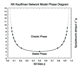
Figure 1: Phase diagram for the Kauffman NK Model in terms of (integer-valued) connectivity $K$ and bit-bias $p$.

One key property of RBNs is the now well established existence of a frozen phase and a chaotic phase  [11, 12] and the critical phase transition lies at the integer value of connectivity $K_{c}=\frac{1}{2p(1-p)}=2$ for unbiased networks with a mean boolean function output value of $p=0.5$. This gives rise to the phase diagram shown in figure 1 which is dominated by the chaotic region and for which simulations are limited to the integer $K$ values shown. It has therefore been of most interest to study RBNs at or around this critical (integer) value of $K_{c}\equiv 2$. In this paper we explore another mechanism to explore the critical region by adopting a mixed-K system.

The Random Boolean Network or graph $G$ is expressed as a four-tuple $\mathbf{G}=(V,E,F,x)$ and has $N=|V|=|F|=|x|$ nodes or vertices($V$), and $N_{a}=|E|$ directed edges or arcs, which express the $K_{i}$ inputs for node $i$. Formally we let $\mathbb{F}_{2}=\{0,1\}$ be a bit-field or Galois Field with the $\oplus$ operator defined modulo $2$ and $\mathbb{F}_{2}^{K}$ is the set of all possible vectors of $K$ bits. Vector $x\in{\mathbb{F}}_{2}^{K}$ and $x_{i}$ is then the bit at position $i$.

The Kauffman NK-Model Network is constructed with fixed (integer) $K=1,2,3,..$ and a boolean function $f_{i}\in F$ of $K_{i}$ inputs is assigned to each node. All the nodes of the network carry a boolean variable $x_{i}$ which may be initialised randomly and each of which is updated (usually, but not necessarily) synchronously in time $t$ from its $j$-labelled inputs so that:

$$x_{i}(t)\leftarrow f_{i}\left(x_{j}(t-1)\right),j=1,2,...,K_{i}$$ (1)

The boolean functions $f$ thus map $\mathbb{F}_{2}^{K}\mapsto\mathbb{F}_{2}$. The mapping can be expressed as a truth table and readily implemented as look-up table in a simulation program [13].

Work has been carried out on a number of different time-update mechanisms for boolean networks including asynchronous algorithms [14, 15]. In this paper we consider only synchronous updates where all nodes execute their boolean function once, at the same time, at every time step. Other studies have also considered how noise [16] effect the crossing times between distinct trajectories. In this paper we adhere to the quenched convention whereby node connections are assigned once and for all time, and particular boolean functions are assigned randomly and uniformly to nodes once and for all time.

The NK-network model assigns the $K_{i}$ inputs for node $i$ randomly and with uniform probability across all possible nodes. Even for a large network there is still a non-zero probability of assigning a node as one of its own inputs. In the case of $K_{i}>1$ there is also a possibility of assigning a node $j$ as an input of $i$ more than once. These self-edges and multiple-edges can have a subtle effect on the behaviour of the NK-network model [17].

A significant body of work has now been carried out on the roles of different sub-classes of boolean functions including the so called canalizing functions  [18] and in particular the effect of bit-bias thresholds and frozen or fixed-value boolean functions on particular elements of the network [19]. A network can therefore be restricted to only have some subset of the possible boolean functions. In the work we describe here, we use network sizes large enough to sample all possible $K$-input boolean functions for the largest $K$ present in the system.

An important consequence of the boolean functions in RBNs is the formation of attractor basins  [20]. These are observed in RBN models whereby diverse initial starting conditions will still lead to statistically similar behaviour. The state of the network falls into attractor cycles whereby a chain of interdependence of nodes (via their boolean functions) leads to the network periodically repeating its state. The number and length of these periods or attractors is of great importance in understanding the behaviour of the NK-model and associated application problems. This can be seen quantitatively by tracking a metric such as changes in the normalised Hamming distance between the network’s successive boolean states. We discuss this metric in section 2.

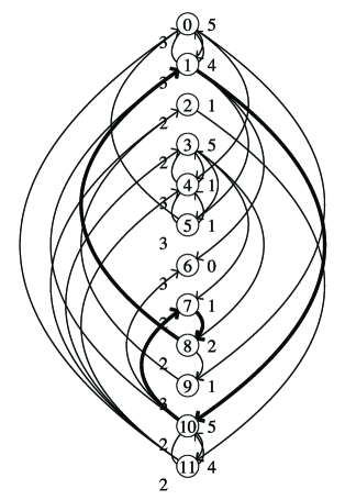
Figure 2: $12$ Node Network, with $\left<K\right>\approx 2.5$. For each node, input degree is shown on the left and output degree is shown on the right. One particular circuit, 1-10-7-8-1, is shown.

Of particular recent interest in the literature has been the uncertainty concerning the number of attractors  [21, 22] and how their number and lengths varied with the size of the network. Scaling was initially believed to be $O(\sqrt{N})$  [23]. It was later reported as linear  [24], and then as “faster than linear”  [25] and subsequently as “stretched exponential” in  [26, 27] but is now known to be faster than any power law  [28].

A recent review of the RBN model  [8] discusses the attractor behaviour in terms of the loops of boolean variable states that form and several exact results concerning these loops have been obtained for the case of connectivity $K\equiv 1$  [29]. Important observations concern the distribution of components with particular sub-classes of possible boolean functions. These “relevant elements” are defined as those nodes that are not frozen and that control at least one other relevant element in the system  [27]. A number of important results have been obtained using particular sub-classes of the possible boolean functions. Drossel et al. [22] have considered networks with non-fixed boolean functions thus making all elements relevant and have therefore shown the equivalence of $K=1$ and $K=2$ networks under appropriate restrictions on the boolean functions.

In this paper we use numerical methods to investigate the role that structural circuits play in the complex structure of the network and the resulting attractor behaviour of RBNs both for mono-$K$ and mixed-$K$ network systems.

Recent work in the literature has used trajectory sampling to study attractor behaviour. The combinatorics of RBN models means that the number of boolean functions grows as $2^{2^{K}}$ with a consequent rapid growth in the number of possible network states with network size. Taking limited numbers of sample trajectories through this state space can lead to very misleading results. Numerical sub-sampling of attractor trajectories seems to be the main difficulty behind obtaining a good understanding of attractor scaling. In this paper we explore the structural properties of RBNs including the number and length distribution of elementary circuits and of components. We compute these properties exactly using brute force enumeration techniques for a range of network sizes and connectivities. Our statistical sampling is only over different randomly configured networks, not over attractor trajectories.

We have found it necessary to study quite large samples (up to 100,000) of networks of size up to 250,000 nodes. The network size $N$ must be at least large enough to adequately sample all possible $K$-input boolean functions for the largest $K$ present in our mixed systems. There are some good software tools available for experimenting with RBNs such as those of Gershenson [7] and Wuensche’s DDLab [30], but we were forced to develop our own custom D code to simulate very large-scale systems [13].

The so-called “edge of chaos” regime [2] is quite narrow when $K$ is restricted to integer values. In this paper we also consider other ways to explore the model phase space. We explore a mixed-$K$ system which we refer to as the $N\left<K\right>$ Network model, with the understanding that although individual nodes (must) have an integer $K$ number of inputs, the system as a whole can have a mean, or effective, $K$ value if there is a distribution of nodes each with different number $K$ of inputs. It then becomes a matter of deciding on a sensible K-distribution for a given model system.

Although some work has been done developing simulations that employ mixed-K models with Poisson or other distributions  [30] we believe no one has yet studied mixed models in systematic detail and furthermore, that our pair-wise model is a novel way of achieving a definite $K_{\mbox{eff}}$. In  [31] Skarja et al. employed a skewed binomial distribution of $K$ values and found an enhanced tendency to orderliness (stability) but based their study of attractors on trajectory sampling.

It is not altogether obvious what the meaning of a distribution in $K$ might mean if it has a long tail with values at high and low $K$ relative to the mean, such as the Poisson distribution in node outputs that results from the mono-K NK model. Consequently we have chosen to study a pair-wise model that generates a $K$ value for each node that interpolates between a pair of integer $K$ values. We define a parameter $P$ that is the linear probability of a node having $K=K_{2}$ rather than $K=K_{1}$. So the cases $P=0$ or $P=1$ correspond to the pure integer states of all nodes having $K_{2}$ or $K_{1}$ respectively, and $P=0.5$ constitutes an equal mix of the designated pair of $K$ values. This means we can approach the transitional value of $K=2$ from above or below and also means we can explore properties with K-dependent relationships thoroughly over a larger range of fractional $K$ values rather than just the small subset of (small) integer $K$ values that is feasible numerically.

Figure 2 shows a small network generated with our mixed pair model. Nodes have 2 or 3 inputs but can have zero or more outputs depending upon the random distribution used during construction in the normal way for NK networks.

In  [17] we explored the behaviour of the growth of the number of elementary circuits and the resulting circuit length distributions in integer $K$-valued NK networks. We suggested that the number of circuits gave a lower bound on the number of attractors present in the associated NK network model. Our numerical experiments exactly enumerated the circuits in various NK networks, without resorting to trajectory sampling and we concluded that the growth in the number of attractors had to be at least as fast as exponential in network size $N$. This clarified some of the recent controversy concerning the growth rates in the number of attractors.

In our earlier work we had an insufficient range of $K$ values to determine a circuit growth relationship with $K$. In this present paper we have sampled higher $K$ values and also examined the pair-wise or fractional $K$ model over a large range of $K$ values and have therefore been able to determine likely relationships between $K$ and the growth of the number of circuits with network size $N$.

We have also observed long-time variations in the normalised Hamming distance for various K-valued networks at small and large network sizes. These suggest the very strong importance of adequately sampling all possible Boolean functions for a given $K$ value. This phenomenon may also explain the anomalous and misleading results on attractor growth obtained from sampling trajectories in too-small networks.

In section 2 we discuss the pair-wise $K$ model and implementation issues. We summarise the the role circuits appear to play in Kauffman nets in section 3 and their enumeration in section 4. In section 5 we present results on the number of circuits and their length distribution both for integer and fractional $K$ network systems. In sections 6 and  7 we offer some discussion of the results and conclusions concerning circuit growth with $K$ and $N$ and the properties of the mixed-pair $K$ model.

2 $K$ Pairs and the $N\left<K\right>$ Model

The conventional Kauffman NK model with mono-K can be extended to a system with a distribution of K-input nodes. RBN simulation tools like Wuensche’s DDLab [30] do make provision for this but it is unclear how to systematically investigate possible distributions, particularly when large samples are required. We might intuit that the mean or effective $K$ value for the whole system plays an important role, but it is not clear how smeared-out any behaviour might be that results from multiple $K$ values. Our pair-wise model approaches the critical value in $K$ from either side by adopting a simple uniform mix of just two possible values of $K$. Most useful are $K=2,3$ and $K=1,2$ to approach $K_{c}\equiv 2$ from above or below, respectively.

An effective-$K$ for the whole network can be defined as:

$$K_{\mbox{eff}}=\left<K_{i}\right>=(1-P).K_{\mbox{low}}+P.K_{\mbox{high}}$$ (2)

where any individual node $i$ has an integer valued number of exactly $K_{i}$ inputs and the average is over all $N$ nodes. Individual nodes are randomly assigned (once and for all time) their particular $K$ value.

We can investigate both static and dynamic properties of this simple mixed model. Static properties are measured from simple graph analysis, and dynamics can be obtained by examining the Normalised Hamming distance between subsequent bit states of the networks’ nodes.

If we have the vector $x\in{\mathbb{F}}_{2}^{K}$ and $x_{i}$ is the bit at position $i$ in the network, we define the Hamming weight as

$$w_{H}=|\{i|x_{i}\neq 0,i=1,2,...,K\}|$$ (3)

and the Hamming distance between two vectors $x,y$ as

$$H_{d}(x,y)=w_{H}(x\oplus y)$$ (4)

It is useful to normalise this by the network size $N$. Of particular interest is the Hamming distance between subsequent states of the network. This is easily calculated as $1-a_{\mbox{same}}$ where $a_{\mbox{same}}$ is the fraction of nodes that have the same bit value at subsequent steps or the single-step correlation function.

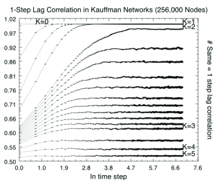
Figure 3: Single-Step lag correlation function (or fraction $a_{\mbox{same}}$) for $256,000$ Node Kauffman Networks for $K=0,1,2,3,4,5$ and networks with mixed pairs of $K$ values in between. This is the same as “one minus the normalised Hamming distance.”

Figure 3 shows the single step correlation function as measured from a variety of different K values. At low-K the network is barely connected and it very rapidly converges to a fixed Boolean state. In highly connected networks the attractor loops (of various lengths) introduce periodic cycles of correspondingly varied frequencies. Nevertheless the mean state of the network still converges to a stable value that depends critically upon $K$.

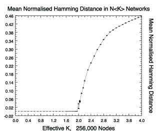
Figure 4: Normalised Hamming long term mean values

Figure 4 shows the long-term mean convergent values of the Normalised Hamming distance $\lim_{t\rightarrow\infty}H_{d}^{1}$ between subsequent (ie time difference of 1) Boolean states of the network as it varies with mean $K$ in our $N\left<K\right>$ model. These are measured for 10 separate samples of an $N=256,000$ node network. We observed that a stable reproducible long-term convergence value is obtained for each K-valued network only if $N$ is significantly larger than the corresponding number $N_{B_{f}}=2^{2^{K}}$ of possible Boolean functions. Not unreasonably, if $N$ is smaller than $N_{B_{f}}$, then the network instantiation is not adequately sampling the Boolean function space. Empirically we found $N>4N_{B_{f}}$ suffices to ensure a reasonable sample. Individual networks generally converge to a stable value within a few hundred time steps. To avoid possible lack of convergence we discarded the first $N$ time steps and averaged over a subsequent $N$ steps. The average has to be taken over a time larger than any likely attractor traversal times present.

Figure 4 does show a very clear transition at $K=2$ as expected for the integer-K $NK$ model, but also indicates that the normalised Hamming distance changes smoothly for the $N\left<K\right>$ model as we vary $K$. This suggests our pair-wise model is indeed a useful way to investigate meaningful non-integer K-valued systems. Intuitively we might expect that $H_{d}^{1}(K-K_{c})$ might have a straight-forward power or other closed function relationship with $\left<K\right>$, but we were not able to obtain a good numerical fit to any obvious forms.

3 Structural Circuits and Attractors

Figure 2 shows a 12-node mixed-K network with $K_{i}\in{2,3}$, $K_{\mbox{eff}}=2.5$ and where the construction algorithm has allowed self-arcs - in other words the inputs for each node have been chosen according to a flat uniform distribution so they can connect to themselves. The consequent self-edges allow self-inputs in the corresponding RBN. These are known to play a vital role in supporting the number of attractors. A self-input or “self-ancestor” in the input dependence chain of boolean variables anchors the periodic or attractor behaviour [8] of RBNs.

We felt intuitively that the presence of structural circuits would also be vital to the periodic attractor behaviour and as Drossel et al. have shown there are definite relationships between the number of attractors and the number of loops. In fact, the number of structural circuits provides a lower bound on the number of possible attractors. Consideration of the exact number of enumerated circuits, and their distribution, gives insight into the controversy over the number of attractors in RBNs.

An elementary circuit is a closed path along a subset of the edges of the graph such that no node, apart from the first and last, appears twice. The number of elementary circuits for a fully connected graph is bounded by

$$\sum_{i=1}^{N-1}C_{N-i+1}^{N}(N-i)!$$ (5)

as given by Harary [32]. This expression therefore represents the limit for the number of structural circuits in an NK-network when $K\rightarrow N$.

Figure 2 shows one such circuit or loop in the network structure. In fact, exact enumeration (as shown in figure 5) indicates that there are 30 arcs and 28 circuits, the longest of which is of length 10. It has 4 self-arcs (and hence two circuits are duplicated) and 3 multiple arcs. The maximum number of outputs is 5 and the minimum is zero. If self-edges are disallowed we would obtain a higher number of circuits present in the network.

  0  0
  0  1  5  0
  0  1 10  7  8  9  2 11  0
  0  1 10  7  8  9  2 11  3  5  0
  0  1 10  7  8  9  2 11  3  5  0
  0  1 10 11  0
  0  1 10 11  3  5  0
  0  1 10 11  3  5  0
  0  9  2 11  0
  0  9  2 11  3  5  0
  0  9  2 11  3  5  0
  0  9  2 11  3  7  8  1  5  0
  0  9  2 11  3  8  1  5  0
  0  9  2 11  0
  0  9  2 11  3  5  0
  0  9  2 11  3  5  0
  0  9  2 11  3  7  8  1  5  0
  0  9  2 11  3  8  1  5  0
  1 10  1
  1 10  7  8  1
  1 10 11  3  7  8  1
  1 10 11  3  8  1
  2 11  2
  2 11  3  7  8  9  2
  2 11  3  8  9  2
  3  3
  4  4
 10 10

Figure 5: Enumerated circuits for the network shown in figure 2.

4 Circuit Enumeration

Various algorithms have been formulated to count the circuits in a graph but these either use infeasible amounts of memory or are time exponential  [33, 34] with a time bound of

$$O(N.e(c+1))$$ (6)

We count circuits using a variation of Johnson’s algorithm  [35] implemented in D. For graphs of $N$ vertices, $e$ edges, $c$ circuits and $1$ fully connected component, Johnson’s algorithm is time bounded in time by

$$O\left((N+e)(c+1)\right)$$ (7)

and space bounded by $O(N+e)$. Unlike Johnson’s algorithm our code copes with partially connected graphs without resorting to the need to treat each of the possible $N_{c}>1$ components separately [36]. This is still a highly expensive process since the number of circuits $c$ itself grows very rapidly with $(N,e)$.

In the graph literature the term loop is unfortunately sometimes used to describe a self-edge or a circuit of length 1. In the NK-networks we study the number of self-edges is much less than $N$, even for low $K$. However we do count them and observe the effect of allowing them in the number of possible circuits and their length histograms. We have extended Johnson’s published algorithm to cope with graphs with directed arcs (and not just bi-directional edges); with multiple components; and self-arcs. The computational complexity is not changed although we store some additional book-keeping information to support arcs. At worst this doubles the memory space required. All the work we report in this present paper is compute-time bound and not space bound.

On a modern (circa 2007) compute server with 4GBytes memory and a speed of 2.66GHz, we found it was entirely feasible to enumerate circuits exactly in networks of up to $N\approx 140$ for $K=1,2$. Smaller networks were required for higher $K$. We were able to count components quite easily up to networks of around $N\approx 20,000$. We were able to exploit the near-linear speed-up of parallel job-farming to average our exact enumeration/counting results over many independently generated networks.

In a detailed investigation of elementary circuits in the graph structure of NK networks [17] we found numerical evidence for rapid growth of the number of circuits with network size N, but were unable to determine a reliable numerical relationship for growth in terms of $K$. This is largely because with integer $K$ we are restricted to only a very few practical values. It is only feasible to study networks up to around $K\approx 9$. This situation is not likely to change even with linear improvement in computer speeds or other supercomputing techniques since the growth in the number of circuits with $K$ scales so rapidly.

Using the mixed model however, we are able to investigate intermediate values in K-space and attempt to find an empirical relationship for circuit growth with $N$ for different mean values of $K$.

5 Circuit Measurement Results

In this section we present results of various numerical experiments, exactly enumerating the circuits over independently generated sample networks. We emphasise that these data are not based on sampling attractor trajectories.

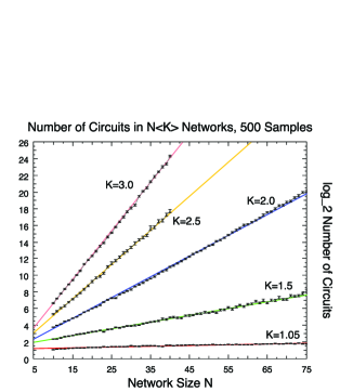
Figure 6: Number of circuits in Mixed-K Networks, sampled over 500 networks.

Figure 6 shows the number of circuits in mixed-K networks, sampled over 500 different networks. Above a $K$ value of 1.5 a straight line fit to $\log N_{c}$ vs $N$ is a good model for the data, whereas for low K, there appears to be a linear relationship between $\log N_{c}$ and $\log N$, as shown in figure 7.

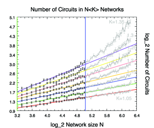
Figure 7: Number of circuits in Mixed-K Networks, sampled over 500 networks.

As we conjectured in [17] there is a definite change in behaviour between the low-K and high-K regimes, however this transition is not a simple one arising from the percolation transition at $K=1$, as figure 7 indicates.

We can explore this effect further by examining the least-squares fitted slopes obtained from figure 6.

Figure 8 shows a straight line fit to these fitted slopes from the data in figure 6 suggesting that the relationship $N_{c}\approx 2^{s.N}$ holds where $s=s(K)$ and for $K>1.5$ this is well fitted by a straight line so that $s\approx 0.340K$ and hence $N_{c}\approx A_{c}2^{0.340K.N}$ holds.

Discounting the effect of self-arcs which grow in number linearly with $N$, and of multiple-arcs which grow with $N^{2}$, the mean number of connections $N_{A}$ is approximately $K.N$ and therefore above $K=1.5$ the model data strongly supports growth in the number of circuits with $N_{A}$

However, figure 8 indicates a very clear departure from this behaviour at $K\approx 1.5$. Interestingly the integer-K NK Kauffman model exhibits a transition in the long term Normalised Hamming distance at $K=2$, as indeed does our mixed-K model as shown in figure 4.

As the error bars in figure 8 show the data does support a straight line fit, although one could convince oneself there is a small anomaly at the critical $K=K_{c}=2$. This is not surprising given the pairwise nature of our mixed model. We are essentially approaching $K_{c}$ independently from above and below. In the case of approach from above we have a system whose nodes mostly have $K=2$ with a few of $K=3$ whereas from below we mix in a minority with $K=1$. It is in fact perhaps a point in favour of the simple pair-wise model that the two curves meet so closely.

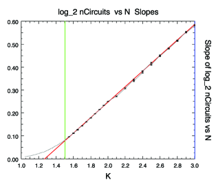
Figure 8: Circuit Slopes of $log_{2}nCircuits$ vs $N$; fitted gradient is 0.340. Experimental data follows the curve shown, with a dark fitted straight line. Error bars were computed from standard deviations and are as shown.

It is also instructive to examine the distribution of circuit lengths present in a typical system.

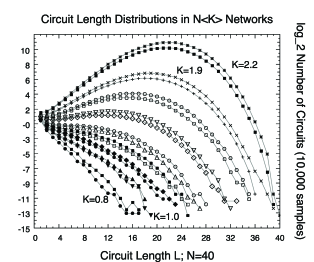
Figure 9: Distribution of circuit lengths in mixed $K$ systems, for fixed network size $N=40$.

Figure 9 shows the length distribution of circuits in networks of fixed $N$ but different $K$. At K values above 1.5, the distribution of circuit lengths has a definite peak around $N/2$ and indicates that there is a non zero, however small, possibility of Hamiltonian or near Hamiltonian circuits present in the system that include all $N$ nodes. Below $K=1.5$ however the circuits length distribution falls monotonically with length and there is no modal length. Although we can only study relatively small network sizes in detail, we might expect that the fall off means there would be almost no circuits of length greater than $N/2$ in large networks, and certainly, that the probability of there being any Hamiltonian circuits is vanishingly small.

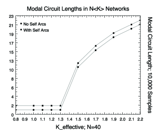
Figure 10: Modal Circuit lengths for 10,000 $N=40$ sample networks as it varies with $K_{\mbox{eff}}$. Note separate curves for networks with and without self-arcs.

Figure 10 shows the modal circuit lengths as they vary with effective $K$ value. Above $K=1.5$ the modal circuit length is non-trivial and grows logarithmically with mean $K$. Below the transition the most likely circuit length present is unity for systems that allow self arcs, and two for systems that do not.

6 Discussion on Network Composition

We have also carried out some standard graph metric analyses on our mixed system to clarify the role of the percolation transition at $K=1$ on the growth circuits. Theoretically we expect that, ignoring the effect of self-arcs and multiple arcs, the percolation transition for infinite sized networks is exactly $K\equiv 1$  [37].

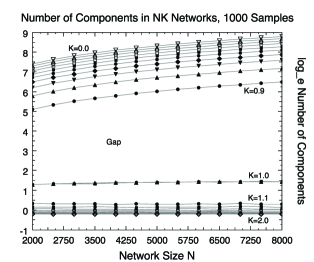
Figure 11: The number of cluster components in a mixed $K$ system for different $K$ and network sizes.

Figure 11 gives some insights into the composition of the system at a mixed value of $K$. At high $K>2$ the system is completely dominated by the single giant component and there are in fact practically no monomers. For $N\gtrsim 2000,K\gtrsim 1$ the number of component clusters is almost identically unity and the number of separate monomers almost identically zero. This transition remains quite sharp in $K$ even for $N\gtrsim 100$ with a clear gap below the critical $K=1$ value.

We found that the average number of monomers is still very small and does not vary with $N$ even for $K>1$. A fully disconnected system with $K\equiv 0$ has each node as a monomer and the number of monomers obviously then grows with $N$. The first intermediate range of $0<K<K_{P}$ shows the system become fully connected, and as discussed, $K_{P}\rightarrow 1$ as $N\rightarrow\inf$, but may be greater than unity for finite $N$. The next intermediate range has $K_{F}<K<K_{c}$ and shows some very interesting changes in the system’s behaviour.

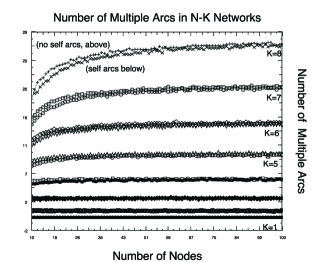
Figure 12: Number of multiple arcs in NK Networks vs network size $N$ for $K=1,2,3,4,5,6,7,8$.

We confirmed empirically our expectation that a system that is constructed to allow self-arcs will exhibit a growth in their number linear in $N$. In the work reported in this paper we have typically experimented with systems both with and without self-arcs. Figure 12 shows a count of the number of multiple arcs and how these are in fact influenced by the presence or absence of self-arcs. For the low-K regimes we are most interested in, the number of multiple arcs is almost invariant with network size, although this does grow logarithmically with $N$ – particularly with high-K. It appears that neither self-arcs nor multiple arcs provide clues to the nature of the $K=1.5$ circuits behaviour transition.

Another graph metric that is computationally inexpensive to compute is the all-pairs distance. Elementary graph textbooks illustrate this for fully connected systems and generally only for bi-directional graphs.

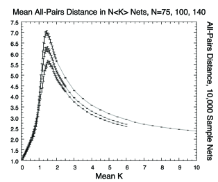
Figure 13: Variation of (modified) mean all pairs distance in mixed $K$ networks for $N=75,100,140$, showing maximal characteristic distance at $K=1.5$.

Figure 13 shows the significance of $K=1.5$ and needs to be carefully interpreted, recalling that it is measuring a bulk graph property across regimes where the graph is neither necessarily fully connected nor fully mutually reachable. As $K$ rises from zero, the $N$ independent nodes become connected and the steepness of rise of the all-pairs distance reaches a maximum at the percolation transition of $K=1$, however even when the network forms a single giant cluster, the connections are directed and not every node is reachable from every other node. Therefore a correct weighted calculation of pair-pair distances, where we include two unreachable nodes as contributing zero rather than infinity, highlights the structural role of connectivity $K=1.5$. At this connectivity the network supports the greatest set of traversal distances present consistent with being a fully connected system. Note further that mutual reachability tails off rather slowly and even at high $K$ there are still “islands of directed disconnection” in the system.

We can further explore the notion of vertex reachability as distinct from connectivity.

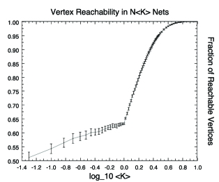
Figure 14: Fraction of Reachable vertices for different $<K>$ showing three regimes: multiple components for $K<1$; one component, but with varying vertex reachability for $1<K\lesssim 6$ and fully connect and fully reachable for large $K$.

Figure 14 shows the fraction of mutually reachable vertices for different mean $K$ in our model, with 560 nodes. At $K<1$ we see multiple disconnected components, but we do not in fact reach full reachability until $K\approx 6$.

Figure 13 also shows the sharpening of the transition with increasing network size. It is worth noting that many of the applications of Kauffman networks as they relate to real physical and biological systems have very definitely finite network sizes $N$ of a few hundred to a few tens of thousands and we are not solely interested in thermodynamically sized systems.

We can verify the bluntening of the percolation transition by counting the fraction of the network nodes in the giant component.

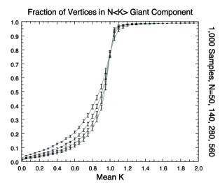
Figure 15: Fraction of vertices in the giant component for different $<K>$ showing a sharpening of the edge for increasing network size $N$.

Figure 15 shows how our network system generation algorithm will produce disconnected clusters even above $K=K_{P}\equiv 1$ for finite network size $N$. We conjectured that the $K=1.5$ transition might be related to partial component disconnection, but even when one edits out everything except the giant components and arranges them by size, we still see this effect within a fully connected component with mean $K=1.5$.

7 Summary and Conclusions

There seems to be several important transition values in the mixed-K model: the percolation transition at $K\approx 1$ from a disconnected to a fully connected system; the structural transition at $K=K_{S}\approx 1.5$ and the Kauffman transition from the stable to chaotic regime at $K_{C}\equiv 2$.

Our study was originally motivated on the assumption that there is a close relationship between the number of elementary circuits in the underpinning structural network and the number of attractors that can be supported in an associated RBN. As Aldana and Cluzel observe [38], the average connectivity $K_{\mbox{eff}}$ appears irrelevant in describing highly heterogeneous scale-free topological regimes of an NK system, but it does appear to be useful in characterising the transitional regime between $K_{P}$ and $K_{c}$.

Specifically, it appears that the structural transition at $K=1.5$ strongly influences the number of possible circuits in the system, but it requires the $K=2$ connectivity transition for the boolean functions to be able to exploit it and to produce a number of attractors that cross into the chaotic phase.

In  [22] Drossel et al. speculate that the vast number of attractors in $NK$ models appear to be a consequence of the synchronous updating scheme. While no doubt the synchronicity plays a role, we believe our work shows that the growth of attractors is also a more fundamental consequence of the structural circuits present in the underpinning $NK$ graph.

We have shown that above $K_{S}$ the number of structural circuits appears to be a relatively simple exponential function of the number of connections $N_{A}$ where discounting self-arcs and multiple arcs, $N_{A}\approx K.N$. This relationship models both the NK Network system and our pair-wise $N\left<K\right>$ system. The number of circuits $N_{C}$ therefore does appear to be a useful lower bound on the number of attractors in both models, and it remains for future work to refine this relationship and bound.

References

- [1] Stuart Kauffman. Homeostasis and differentiation in random genetic control networks. Nature, 224(5215):177–178, October 1969.
- [2] S. A. Kauffman. The Origins of Order. Oxford University Press, 1993.
- [3] Stephen Wolfram. Theory and Applications of Cellular Automata. World Scientific, 1986.
- [4] Stuart Kauffman, Carsten Peterson, Bjorn Samuelsson, and Carl Troein. Random boolean network models and the yeast transcriptional network. Proc. Natl. Acad. Sci. USA, 100:14796, 2003.
- [5] C. F. Baillie and D.A. Johnston. Damaging 2d quantum gravity. Physics Letters B, 326:51–56, 1994.
- [6] C.F. Baillie, K.A. Hawick, and D.A. Johnston. Quenching 2d quantum gravity. Physics Letters B, 328(3-4):284–290, June 1994.
- [7] Carlos Gershenson. Introduction to random boolean networks. Technical Report arXiv.org:nlin/0408006v3, Vrije Universiteit Brussel, August 2004.
- [8] Leo Kadanoff, Susan Coppersmith, and Maximino Aldana. Boolean dynamics with random couplings. In E. Kaplan, J. Marsden, and K. Sreenivasan, editors, Perspectives and Problems in Nonlinear Science. Springer, 2003.
- [9] Jeffrey J. Fox and Colin C. Hill. From topology to dynamics in biochemical networks. Chaos, 11:809–815, 2001.
- [10] J. F. Lynch. Dynamics of random boolean networks. In Proc. Conf on Mathematical Biology and Dynamics Systems, University of Texas at Tyler, 2005.
- [11] B. Derrida and Y. Pomeau. Random networks of automata: A simple annealed approximation. Europhys. Lett., 1(2):45–49, 1986.
- [12] B. Derrida and D. Stauffer. Phase transitions in two-dimensional Kauffman cell automata. Europhys. Lett., 2:739, 1986.
- [13] K.A.Hawick, H.A.James, and C.J.Scogings. Simulating large random boolean networks. Technical Report CSTN-039, Information and Mathematical Sciences, Massey University, Albany, North Shore 102-904, Auckland, New Zealand, May 2007.
- [14] I. Harvey and T. Bossomaier. Time out of joint: Attractors in asynchronous random boolean networks. In P. Husbands and I. Harvey, editors, Proc Fourth European Conference on Artificial Life (ECAL97), pages 67–75. MIT Press, 1997.
- [15] Bertrand Mesot and Christof Teuscher. Critical values in asynchronous random boolean networks. In Evolutionary and Adaptive Dynamics, volume 2801 of LNCS, chapter Critical Values in Asynchronous Random Boolean Networks, pages 367–376. Springer, 2004.
- [16] X. Qu, M. Aldana, and Leo P. Kadanoff. Numerical and theoretical studies of noise effects in the Kauffman model. J. Stat. Phys., 109:967–986, 2002.
- [17] K.A.Hawick, H.A.James, and C.J.Scogings. Structural circuits and attractors in Kauffman networks. In M.Randall, H.Abbas, and J.Wiles, editors, Proc. Australasian Conference on Artificial Life (ACAL), volume 4828 of LNAI, pages 190–201. Springer-Verlag, 2007.
- [18] A. Szejka and B. Drossel. Evolution of canalizing boolean networks. Eur. Phys. J. B, 56:373–380, 2007.
- [19] F. Greil and B. Drossel. Kauffman networks with threshold functions. Eur. Phys. J. B, 57:109–113, 2007.
- [20] A. Wuensche. Discrete dynamical networks and their attractor basins. In R. Standish and et al., editors, Proc. Complex Systems 1998, pages 3–21. UNSW, Sydney, Australia, 1998.
- [21] Barbara Drossel. On the number of attractors in random boolean networks. Technical Report arXiv.org:cond-mat/0503526, Institute fur Festkorperphysik, TU Darmstadt, March 2005.
- [22] Barbara Drossel, Tamara Mihaljev, and Florian Greil. Number and length of attractors in a critical Kauffman model with connectivity one. Phys. Rev. Lett., 94:088701, March 2005.
- [23] S. A. Kauffman. Metabolic stability and epigenesis in randomly constructed genetic nets. Journal of Theoretical Biology, 22:437–467, 1969.
- [24] Sven Bilke and Fredrik Sjunnesson. Stability of the Kauffman model. Phys. Rev. E, 65:016129, 2001.
- [25] J. E. S. Socolar and S. A. Kauffman. Scaling in ordered and critical random boolean metworks. Phys. Rev. Lett., 90:068702–1, 2003.
- [26] U. Bastolla and G. Parisi. Relevant elements, magnetization and dynamical properties in Kauffman networks: A numerical study. Physica D, 115:203–218, 1998.
- [27] U. Bastolla and G. Parisi. The modular structure of Kauffman networks. Physica D, 115:219–233, 1998.
- [28] Bjorn Samuelsson and Carl Troein. Superpolynomial growth in the number of attractors in Kauffman networks. Phys. Rev. Lett., 90:098701–1, 2003.
- [29] H. Flyvbjerg and N. J. Kjaer. Exact solution of Kauffman’s model with connectivity one. J. Phys. A: Math. Theor., 21:1695–1718, 1988.
- [30] Andrew Wuensche. Attractor Basins of Discrete Networks - Implications on self-organisation and memory. PhD thesis, University of Sussex, October 1996.
- [31] Metod Skarja, Barbara Remic, and Igor Jerman. Boolean networks with variable number of inputs (k). Chaos, 14(2):205–216, June 2004.
- [32] Frank Harary and Edgar M. Palmer. Graphical Enumeration. New York, Academic Press, 1973.
- [33] J. C. Tiernan. An efficient search algorithm to find the elementary circuits of a graph. Communications of the ACM, 13:722–726, 1970.
- [34] R. Tarjan. Enumeration of the elementary circuits of a directed graph. SIAM Journal on Computing, 2:211–216, 1973.
- [35] Donald B. Johnson. Finding all the elementary circuits of a directed graph. SIAM Journal on Computing, 4(1):77–84, March 1975.
- [36] K.A.Hawick and H.A.James. A fast code for enumerating circuits and loops in graphs. Technical Report CSTN-013, Massey University, November 2005.
- [37] L. Correale, M. Leone, A. Pagnani, M. Weigt, and R. Zecchina. Core percolation and onset of complexity in boolean networks. Phys. Rev. Lett., 96:018101, January 2006.
- [38] Maximino Aldana and Philippe Cluzel. A natural class of robust networks. Proc. Natl. Acad. Sci. USA, 100(15):9710–8714, July 2003.