The magnetron instability in a pulsar’s cylindrical electrosphere.

Abstract

Context. The physics of the pulsar magnetosphere near the neutron star surface remains poorly constrained by observations. Although about 2000 pulsars have been discovered to date, little is known about their emission mechanism, from radio to high-energy X-ray and gamma-rays. Large vacuum gaps probably exist in the magnetosphere, and a non-neutral plasma partially fills the neutron star surroundings to form an electrosphere.

Aims. In several previous works, we showed that the differentially rotating equatorial disk in the pulsar’s electrosphere is diocotron unstable and that it tends to stabilise when relativistic effects are included. However, when approaching the light cylinder, particle inertia becomes significant and the electric drift approximation is violated. In this paper, we study the most general instability, i.e. by including particle inertia effects, as well as relativistic motions. Electromagnetic perturbations are described in a fully self-consistent manner by solving the cold-fluid and Maxwell equations. This general non-neutral plasma instability is called the magnetron instability by plasma physicists.

Methods. We linearise the coupled relativistic cold-fluid and Maxwell equations. The non-linear eigenvalue problem for the perturbed azimuthal electric field component is solved numerically with standard techniques for boundary-value problems like the shooting method. The spectrum of the magnetron instability in a non-neutral plasma column confined between two cylindrically conducting walls is computed for several cylindrical configurations. For a pulsar electrosphere, no outer wall exists. In this case, we allow for electromagnetic wave emission propagating to infinity.

Results. First we checked our algorithm in the low-density limit. We recover the results of the relativistic diocotron instability. When the self-field induced by the plasma becomes significant, it can first increase the growth rate of the magnetron instability. However, equilibrium solutions are only possible when the self-electric field, measured by the parameter $s_{\rm e}$ and tending to disrupt the plasma configuration, is bounded to an upper limit, $s_{\rm e,max}$. For $s_{\rm e}$ close to but smaller than this value $s_{\rm e,max}$, the instability becomes weaker or can be suppressed as was the case in the diocotron regime.

Conclusions. When approaching the light-cylinder, particle inertia becomes significant in the equatorial disk of the electrosphere. Indeed, the rest-mass energy density of the plasma becomes comparable to the magnetic energy density. The magnetron instability sets in and takes over the destabilisation of the stationary flow initiated by the diocotron instability close to the neutron star surface. As a consequence, the flow in the pulsar inner magnetosphere is highly unstable, leading to particle diffusion across the magnetic field line. Therefore, an electric current can circulate in the closed magnetosphere and feed the wind with charged particles.

1 INTRODUCTION

This year, we celebrate the 40th year of the discovery of the first pulsar. Nevertheless, the detailed structure of charge distribution and electric-current circulation in the closed magnetosphere of a pulsar remains poorly understood. Although it is often assumed that the plasma fills the space entirely and corotates with the neutron star, it is on the contrary very likely that it only partly fills it, leaving large vacuum gaps between plasma-filled regions. The existence of such gaps in aligned rotators has been very clearly established by Krause-Polstorff & Michel (1985a, b). Since then, a number of different numerical approaches to the problem have confirmed their conclusions, including some work by Rylov (1989), Shibata (1989), Zachariades (1993), Neukirch (1993), Thielheim & Wolfsteller (1994), Spitkovsky & Arons (2002), and ourselves (Pétri et al., 2002b). This conclusion about the existence of vacuum gaps has been reached from a self-consistent solution of the Maxwell equations in the case of the aligned rotator. Moreover, Smith et al. (2001) have shown by numerical modelling that an initially filled magnetosphere like the Goldreich-Julian model evolves by opening up large gaps and stabilises to the partially filled and partially void solution found by Krause-Polstorff & Michel (1985a) and also by Pétri et al. (2002b). The status of models of the pulsar magnetospheres, or electrospheres, has recently been critically reviewed by Michel (2005). A solution with vacuum gaps has the peculiar property that those parts of the magnetosphere that are separated from the star’s surface by a vacuum region are not corotating and so suffer differential rotation, an essential ingredient that will lead to non-neutral plasma instabilities in the closed magnetosphere, a process never addressed in detail.

This raises the question of the stability of such a charged plasma flow in the pulsar magnetosphere. The differential rotation in the equatorial, non-neutral disk induces a non-neutral plasma instability that is well known to plasma physicists (Oneil 1980; Davidson 1990; O’Neil & Smith 1992). Their good confinement properties (trapped particles can remain on an almost unperturbed trajectory for thousands of gyro-periods) makes them a valuable tool for studying plasmas in laboratory, by using for instance Penning traps. In the magnetosphere of a pulsar, far from the light cylinder and close to the neutron star surface, the instability reduces to its non-relativistic and electrostatic form, the diocotron instability. The linear development of this instability for a differentially rotating charged disk was studied by Pétri et al. (2002a), in the thin disk limit, and by Pétri (2007a, b) in the thick disk limit. It both cases, the instability proceeds at a growth rate comparable to the star’s rotation rate. The non-linear development of this instability was studied by Pétri et al. (2003), in the framework of an infinitely thin disk model. They have shown that the instability causes a cross-field transport of these charges in the equatorial disk, evolving into a net out-flowing flux of charges. Spitkovsky & Arons (2002) have numerically studied the problem and concluded that this charge transport tends to fill the gaps with plasma. The appearance of a cross-field electric current as a result of the diocotron instability has been observed by Pasquini & Fajans (2002) in laboratory experiments in which charged particles were continuously injected in the plasma column trapped in a Malmberg-Penning configuration.

A general overview of the equilibrium and stability properties of non-neutral plasmas in Cartesian and cylindrical geometry can be found in Davidson et al. (1991). Tsang & Davidson (1986) describe how to compute fully self-consistent general equilibria configuration for a cold-fluid plasma in a cylindrical diode. This is useful to investigate the stability properties in magnetron devices as presented in Davidson & Tsang (1986).

The aim of this work is to extend the previous work by Pétri (2007a, b) on the diocotron instability by including particle inertia effects. In this paper we present a numerical analysis of the linear growth of the relativistic magnetron instability for a non-neutral plasma column. The paper is organised as follows. In Sect. 2, we describe the initial setup of the plasma column consisting of an axially symmetric equilibrium between two conducting walls. We give several equilibrium profiles useful for the study of the magnetron instability in different configurations. In Sect. 3, the non-linear eigenvalue problem satisfied by the perturbed azimuthal electric field component is derived. The algorithm to solve the eigenvalue problem is checked against known analytical results in the low-density limit (diocotron instability), Sect. 4. Then, applications to some typical equilibrium configurations are shown in Sect. 5. First we consider a plasma column with constant density. Next, we study the effect of the cylindrical geometry (curvature of the flow) and the transition to the planar diode limit. Finally, the consequences of the magnetron instability on the pulsar electrosphere is investigated. The conclusions and the possible generalisation are presented in Sect. 6.

2 THE MODEL

We study the motion of a non-neutral plasma column of infinite axial extend along the $z$-axis. We adopt cylindrical coordinates denoted by $(r,\varphi,z)$ and define the corresponding orthonormal basis vectors by $(\@vec{e}_{\rm r},\@vec{e}_{\rm\varphi},\@vec{e}_{\rm z})$. The geometric configuration is the same as the one described in our previous works (Pétri 2007a, b).

In this section, we briefly summarise the equilibrium conditions imposed on the plasma and give some typical examples of equilibrium configurations for specified velocity, density and electric field profiles.

We consider a single-species non-neutral plasma consisting of particles with mass $m_{\rm e}$ and charge $q$ trapped between two cylindrically conducting walls located at the radii $W_{1}$ and $W_{2}>W_{1}$. The plasma column itself is confined between the radii $R_{1}\geq W_{1}$ and $R_{2}\leq W_{2}$, with $R_{1}<R_{2}$. This allows us to take into account vacuum regions between the plasma and the conducting walls. Because we solve the full set of Maxwell equations, there is also the possibility for the plasma to radiate electromagnetic waves to infinity. In order to take this effect into account, we remove the outer wall if necessary and replace it by outgoing wave boundary conditions at $R_{2}$.

2.1 Equations of motion

Let us describe the equation of motion satisfied by the plasma column. Each particle evolves in the self-consistent electromagnetic field partly imposed by an external device and partly induced by the plasma itself. The motion of the plasma column is governed by the cold-fluid equations, i.e. the conservation of electric charge and the conservation of momentum, respectively,

$$\frac{\partial\rho_{\rm e}}{\partial t}+{\rm div}\,(\rho_{\rm e}\,\@vec{v}) = 0$$ (1)

$$\left(\frac{\partial}{\partial t}+\@vec{v}\cdot\frac{\partial}{\partial\@vec{r}}\right)(\gamma\,m_{\rm e}\,\@vec{v}) = q\,(\@vec{E}+\@vec{v}\wedge\@vec{B})$$ (2)

We introduced the usual notation, $\rho_{\rm e}$ for the electric charge density, $\@vec{v}$ for the velocity, $(\@vec{E},\@vec{B})$ for the electromagnetic field. The Lorentz factor of the flow is $\gamma=1/\sqrt{1-\@vec{v}^{2}/c^{2}}$. Eqs. (1) and (2) are supplemented by the full set of Maxwell equations,

$$\@vec{\rm rot}\,\@vec{E} = -\frac{\partial\@vec{B}}{\partial t}$$ (3)

$$\@vec{\rm rot}\,\@vec{B} = \mu_{0}\,\@vec{j}+\varepsilon_{0}\,\mu_{0}\,\frac{\partial\@vec{E}}{\partial t}$$ (4)

$${\rm div}\,\@vec{E} = \frac{\rho_{\rm e}}{\varepsilon_{0}}$$ (5)

$${\rm div}\,\@vec{B} = 0$$ (6)

where $\mu_{0}$ is the magnetic permeability and $\varepsilon_{0}$ the electric permittivity. For a non-neutral plasma, the current density corresponds to convective motion in the plasma and is therefore related to the charge density by

$$\@vec{j}=\rho_{\rm e}\,\@vec{v}$$ (7)

The set of Eqs. (1)-(7) represents the most general treatment of the cold fluid behavior, including relativistic and electromagnetic effects as well as inertia of the particles (the electric drift approximation, used to study the diocotron instability, is replaced by Eq. (2)).

2.2 Equilibrium of the plasma column

In equilibrium, the particle number density is $n_{\rm e}(r)$ and the charge density is $\rho_{\rm e}(r)=q\,n_{\rm e}(r)$. Particles evolve in a cross electric and magnetic field such that the equilibrium magnetic field is directed along the $z$-axis whereas the equilibrium electric field is directed along the $r$-axis. On average, the stationary motion is only azimuthal. The electric field induced by the plasma itself is

$$\@vec{E}_{\mathrm{p}} = E_{\rm r}\,\@vec{e}_{\rm r}.$$ (8)

The magnetic field is made of two parts, an imposed external applied field, $\@vec{B}_{0}$, assumed to be uniform in the region outside the plasma column, and a plasma induced field, $\@vec{B}_{\mathrm{p}}$ such that the total magnetic field is

$$\@vec{B}=\@vec{B}_{\mathrm{p}}+\@vec{B}_{0}=B_{\rm z}\,\@vec{e}_{\rm z}.$$ (9)

Therefore, for azimuthally symmetric equilibria, the steady-state Maxwell-Gauss and Maxwell-Ampère equations satisfy

$$\frac{1}{r}\,\frac{\partial}{\partial r}(r\,E_{\rm r}) = \frac{\rho_{\rm e}}{\varepsilon_{0}}$$ (10)

$$\frac{\partial B_{\rm z}}{\partial r} = -\mu_{0}\,\rho_{\rm e}\,v_{\varphi}.$$ (11)

In the stationary state, $\partial/\partial t=0$, the balance between the Lorentz force and the centrifugal force for a fluid element in Eq. (2) is expressed as

$$\gamma\,m_{\rm e}\,\frac{v_{\varphi}^{2}}{r}+q\,(E_{\rm r}+v_{\varphi}\,B_{\rm z})=0.$$ (12)

It is convenient to introduce the non-relativistic plasma and cyclotron frequencies respectively by

$$\Omega_{\rm p}^{2} = \frac{\rho_{\rm e}\,q}{m_{e}\,\varepsilon_{0}}$$ (13)

$$\Omega_{\rm c} = \frac{q\,B_{\rm z}}{m_{e}}$$ (14)

The corresponding relativistic expressions are respectively

$$\omega_{\rm p}^{2} = \frac{\Omega_{\rm p}^{2}}{\gamma}$$ (15)

$$\omega_{\rm c} = \frac{\Omega_{\rm c}}{\gamma}$$ (16)

where $\gamma=1/\sqrt{1-v_{\varphi}^{2}/c^{2}}$ corresponds to the Lorentz factor of the azimuthal flow. The plasma equilibrium is governed by two antagonistic effects. On one hand, the electric field induced by the plasma itself exerts a repelling force on the fluid element, trying to inflate the plasma. On the other hand, the magnetic field confines the plasma by incurving the particle trajectories. To quantify the strength of each effect, focusing magnetic field and defocusing electric field, it is useful to introduce the self-field parameter defined by

$$s_{\rm e}\equiv\frac{\omega_{\rm p}^{2}}{\omega_{\rm c}^{2}}=\gamma\,\frac{\Omega_{\rm p}^{2}}{\Omega_{\rm c}^{2}}$$ (17)

Note that this self-field parameter is a local quantity defined on every point in space as are the plasma and cyclotron frequencies. It can therefore depend on the radius $r$ and is generally not a constant throughout the plasma column. We should write it $s_{\rm e}(r)$ but in order to avoid overloading, we do not explicitly show the space dependence of any quantity as they should all depend on $r$ except otherwise specified. The diocotron regime, or electric drift approximation, corresponds to the low-density limit, i.e. to $s_{\rm e}\ll 1$ in the whole plasma column. We assume that the electric field induced by the plasma vanishes at the inner wall, at $r=W_{1}$, i.e.

$$\@vec{E}_{\mathrm{p}}(W_{1})=\@vec{0}.$$ (18)

Integrating Eq. (10) therefore gives for the electric field generated by the plasma,

$$\@vec{E}_{\mathrm{p}}(r)=\frac{1}{\varepsilon_{0}\,r}\,\int_{W_{1}}^{r}\rho_{\rm e}(r^{\prime})\,r^{\prime}\,dr^{\prime}\,\@vec{e}_{\rm r}$$ (19)

For the magnetic field induced by the plasma, we solve Eq. (11) with the boundary condition $B_{\rm z}(R_{2})=B_{0}$. This simply states that the total magnetic field outside the plasma column has to match the magnetic field imposed by an external device. Integrating within the plasma column, it is given by :

$$B_{\rm z}(r)=B_{0}-\mu_{0}\,\int_{R_{2}}^{r}\rho_{\rm e}(r^{\prime})\,v_{\varphi}(r^{\prime})\,dr^{\prime}$$ (20)

Any equilibrium state is completely determined by the following four quantities, the total radial electric field, $E_{\rm r}$, the total axial magnetic field, $B_{\rm z}$, the charge density, $\rho_{\rm e}$, and the azimuthal speed of the guiding center, $v_{\varphi}$. Prescribing one of these profiles, the remaining three are found self-consistently by solving the set of Eqs. (10), (11) and (12). In the next subsections, we show how to derive these quantities for some typical examples in which either the velocity profile, the density profile or the electric field are imposed.

2.3 Specified velocity profile

Let us first assume that the velocity profile $v_{\varphi}=r\,\Omega$ is prescribed, $\Omega$ being the angular velocity at equilibrium. This case is well-suited for the study of the pulsar’s electrosphere in which the plasma is in differential rotation and evolves in a dipolar magnetic field. As already noticed before, the differential rotation is essential to the presence of the instability. The other equilibrium quantities, $(E_{\rm r},B_{\rm z},\rho_{\rm e})$, are easily derived from $\Omega$. Indeed, inserting $\rho_{\rm e}$ from Eq. (10) and $E_{\rm r}$ from Eq. (12) into Maxwell-Ampère equation (11), the magnetic field satisfies a first order linear ordinary differential equation

$$\frac{\partial B_{\rm z}}{\partial r} = \frac{\gamma^{2}\,\beta}{r}\,\left[B_{\rm z}\,\frac{\partial}{\partial r}(r\,\beta)+\frac{m_{\rm e}\,c}{q}\,\frac{\partial}{\partial r}\left(\gamma\,\beta^{2}\right)\right].$$ (21)

The Lorentz factor of the flow is

$$\gamma = \frac{1}{\sqrt{1-\beta^{2}}}$$ (22)

$$\beta = \frac{r\,\Omega}{c}$$ (23)

From Maxwell-Ampère equation, Eq. (11), the charge density is found by

$$\rho_{\rm e}=-\frac{1}{\mu_{0}\,v_{\varphi}}\,\frac{\partial B_{\rm z}}{\partial r}$$ (24)

The electric field is recovered from the force balance equation, Eq. (12),

$$E_{\rm r}=-\frac{\gamma\,m_{\rm e}\,v_{\varphi}^{2}}{q\,r}-v_{\varphi}\,B_{\rm z}$$ (25)

2.4 Specified density profile

Another interesting case corresponds to a specified charge density profile $\rho_{\rm e}$. Replacing Eq. (19) and (20) into the force balance Eq. (12), the rotation profile is solution of a non-linear Volterra integral equation

$$\frac{r\,\Omega^{2}}{\sqrt{1-r^{2}\,\Omega^{2}/c^{2}}}+\frac{1}{r}\,\int_{W_{1}}^{r}\Omega_{\rm p}^{2}(r^{\prime})\,r^{\prime}\,dr^{\prime}$$

$$+ r\,\Omega\,\left[\Omega_{\rm c0}-\frac{1}{c^{2}}\,\int_{R_{2}}^{r}\Omega_{\rm p}^{2}(r^{\prime})\,\Omega(r^{\prime})\,r^{\prime}\,dr^{\prime}\right]=0$$

$\Omega_{\rm c0}=q\,B_{0}/m_{\rm e}$ is the non-relativistic cyclotron frequency associated to the external magnetic field $B_{0}$. Knowing $\Omega$, the same procedure as in the previous subsection for a specified velocity profile is applied, i.e. the electromagnetic field is calculated according to Eq. (21) and (25).

2.5 Specified electric field

It is also possible to specify the equilibrium radial electric field. An interesting case is given by

$$E_{\rm r}(r)=\left\{\begin{array}[]{lcl}0&,&W_{1}\leq r\leq R_{1}\\ -c\,B_{0}\,\displaystyle{\frac{\sinh\alpha\,(r-R_{1})}{\cosh\alpha\,(R_{2}-R1)}}&,&R_{1}\leq r\leq R_{2}\\ -c\,B_{0}\,\displaystyle{\frac{R_{2}\,\tanh\alpha\,(R_{2}-R1)}{r}}&,&R_{2}\leq r\leq W_{2}\end{array}\right.$$ (27)

$\alpha$ is a constant useful to adjust the maximal speed of the column. The equilibrium electric field profile, Eq. (27), enables us to investigate the influence of the cylindrical geometry compared to the planar diode geometry. Indeed, in the limit of small curvature, $R_{2}-R_{1}\ll R_{1}$, the eigenvalue problem in cylindrical geometry reduces to the planar diode case. The magnetic field is solution of an ordinary differential equation

$$\frac{\partial B_{\rm z}}{\partial r}=-\frac{\beta}{r\,c}\,\frac{\partial}{\partial r}\left(r\,E_{\rm r}\right)$$ (28)

The density is easily found from Maxwell-Poisson Eq. (10) to be

$$\rho_{\rm e} = n_{0}\,q$$

$$= -\frac{\varepsilon_{0}\,B_{0}\,\alpha}{\cosh\alpha\,(R_{2}-R1)}\,\left[\cosh\alpha\,(r-R1)+\frac{\sinh\alpha\,(r-R1)}{\alpha\,r}\right]$$

where $n_{0}$ is the plasma density within the column. Finally, the velocity is given by the centrifugal and Lorentz forces balance, Eq. (12).

3 LINEAR ANALYSIS

In this section, we derive the eigenvalue problem for the magnetron instability in the most general case. We apply the standard linear perturbation theory. All scalar perturbations of a physical quantity $X$ like electric potential, density, and velocity components, are expressed by the expansion

$$X(r,\varphi,t)=X(r)\,e^{i\,(l\,\varphi-\omega\,t)}$$ (30)

where $l$ is the azimuthal mode and $\omega$ the eigenfrequency. A more general treatment of the perturbation in full 3D allowing for a stratified vertical structure of the plasma column would need to introduce a wavenumber $k$, directed along the z-axis, in the phase term, like $(k\,z+l\,\varphi-\omega\,t)$. Techniques to deal with this general expansion are discussed in Sect. 3.1 of Pétri (2007a).

The decomposition in Eq. (30) only allows for a global mode to propagate in the plasma. The frequency does not depend on the radius. Nevertheless, we could imagine to split the column of plasma in different annular layers $L_{i}$, let us say $N$ layers such that $i\in[[1..N]]$. Each of them possesses its own eigenfrequency $\omega_{i}$. Then, by using matching conditions at the interface between successive layers, we could solve the eigenvalue problem and compute the radius dependent growth rates. This would be a generalisation of the technique employed to match the vacuum solution to the plasma column as described below.

3.1 Linearisation of Maxwell equations

We study the stability of the plasma column around the equilibrium mentioned in Sect. 2. An expansion to first order of the electromagnetic field around this equilibrium $(\@vec{E}^{0},B_{\rm z}^{0})$ leads to

$$\@vec{E} = \@vec{E}^{0}+\delta\@vec{E}$$ (31)

$$B_{\rm z} = B_{\rm z}^{0}+\delta B_{\rm z}$$ (32)

and the same for the charge and current densities

$$\@vec{j} = \@vec{j}^{0}+\delta\@vec{j}$$ (33)

$$\rho_{\rm e} = \rho_{\rm e}^{0}+\delta\rho_{\rm e}$$ (34)

Linearising the set of Maxwell equations, (3)-(6), we have

$$\frac{1}{r}\,\frac{\partial}{\partial r}(r\,\delta\,E_{\rm r})+i\,\frac{l}{r}\,\delta E_{\varphi} = \frac{\delta\rho_{\rm e}}{\varepsilon_{0}}$$ (35)

$$\frac{1}{r}\,\frac{\partial}{\partial r}(r\,\delta\,E_{\varphi})-i\,\frac{l}{r}\,\delta E_{\rm r} = i\,\omega\,\delta B_{\rm z}$$ (36)

$$i\,\frac{l}{r}\,\delta B_{\rm z} = \mu_{0}\,\delta j_{\rm r}-i\,\frac{\omega}{c^{2}}\,\delta E_{\rm r}$$ (37)

$$-\frac{\partial}{\partial r}\delta B_{\rm z} = \mu_{0}\,\delta j_{\varphi}-i\,\frac{\omega}{c^{2}}\,\delta E_{\varphi}$$ (38)

The current density perturbation is

$$\delta j_{\rm r} = \rho_{\rm e}\,\delta v_{\rm r}$$ (39)

$$\delta j_{\varphi} = \delta\rho_{\rm e}\,v_{\varphi}+\rho_{\rm e}\,\delta v_{\varphi}$$ (40)

It is convenient to introduce a potential $\delta E_{\varphi}=-i\,l\,\phi/r$ (we emphasise that this function is not the scalar potential from which the electric field could be derived, but is just a convenient auxiliary variable) such that the electric and magnetic field become

$$\delta E_{\rm r} = -\kappa\,\left[\frac{\partial\phi}{\partial r}-i\,\mu_{0}\,\omega\,\frac{r^{2}}{l^{2}}\,\rho_{\rm e}\,\delta v_{\rm r}\right]$$ (41)

$$\delta B_{\rm z} = \frac{\omega\,r}{l}\,\kappa\,\left[\frac{1}{c^{2}}\,\frac{\partial\phi}{\partial r}-i\,\frac{\mu_{0}}{\omega}\,\rho_{\rm e}\,\delta v_{\rm r}\right]$$ (42)

$$\kappa = \frac{1}{1-(\omega\,r/l\,c)^{2}}$$ (43)

Maxwell-Gauss equation, (5), is therefore written

$$\frac{1}{r}\,\frac{\partial}{\partial r}\left(r\,\kappa\,\frac{\partial\phi}{\partial r}\right)-\frac{l^{2}}{r^{2}}\,\phi=-\frac{\delta\rho_{\rm e}}{\varepsilon_{0}}\,+i\,\mu_{0}\,\frac{\omega}{r}\,\frac{\partial}{\partial r}\left(\frac{r^{3}}{l^{2}}\,\kappa\,\rho_{\rm e}\,\delta v_{\rm r}\right)$$ (44)

In order to find the eigenvalue equation satisfied by the function $\phi$, we have to relate the density and velocity perturbations, $\delta\rho_{\rm e}$, $\delta v_{\rm r}$ and $\delta v_{\varphi}$, to $\phi$. These expressions are derived in the next paragraph.

3.2 Linearisation of the fluid equations

Linearising the conservation of momentum, Eq. (2), the radial and azimuthal perturbations in velocity are related to the perturbation in electromagnetic field as follows

$$-i\,(\omega-l\,\Omega)\,\delta v_{\rm r}-(\omega_{\rm c}+2\,\Omega_{\rm b})\,\delta v_{\varphi} =$$

$$\frac{q}{\gamma\,m_{\rm e}}\,(\delta E_{\rm r}+r\,\Omega\,\delta B_{\rm z})-i\,(\omega-l\,\Omega)\,\gamma^{2}\,\delta v_{\varphi}$$

$$-\left(\omega_{\rm c}+\frac{1}{\gamma\,r}\,\frac{\partial}{\partial r}(r^{2}\,\gamma\,\Omega)\right)\,\delta v_{\rm r} = \frac{q}{\gamma\,m_{\rm e}}\,\delta E_{\varphi}$$ (45)

Following Davidson & Tsang (1986), we introduced the Coriolis frequency

$$\Omega_{\rm b}=\frac{1+\gamma^{2}}{2}\,\Omega$$ (46)

From Eqs. (41) and (42), we find

$$\delta E_{\rm r}+r\,\Omega\,\delta B_{\rm z}=-\kappa\,\left[\left(1-\frac{\omega\,r}{l\,c}\,\frac{\Omega\,r}{c}\right)\,\frac{\partial\phi}{\partial r}-i\,\mu_{0}\,\rho_{\rm e}\frac{r^{2}}{l^{2}}\,(\omega-l\,\Omega)\,\delta v_{\rm r}\right]$$ (47)

From the continuity equation, (1), we get

$$\delta\rho_{\rm e}=\frac{1}{i\,(\omega-l\,\Omega)}\,\left[\frac{1}{r}\,\frac{\partial}{\partial r}(r\,\rho_{\rm e}\,\delta v_{\rm r})+i\,\frac{l}{r}\,\rho_{\rm e}\,\delta v_{\varphi}\right]$$ (48)

Introducing the function

$$\Delta = (\omega_{\rm c}+2\,\Omega_{\rm b})\,\left(\omega_{\rm c}+\frac{1}{\gamma\,r}\,\frac{\partial}{\partial r}(r^{2}\,\gamma\,\Omega)\right)$$ (49)

$$- (\omega-l\,\Omega)^{2}\,\gamma^{2}\,\left(1+\kappa\,\frac{\omega_{\rm p}^{2}\,r^{2}}{l^{2}\,c^{2}}\right)$$

we solve for the velocity perturbation as

$$\delta v_{\rm r} = \frac{i\,q}{\gamma\,m_{\rm e}\,\Delta}\,\left[(\omega-l\,\Omega)\,\gamma^{2}\,\kappa\,\left(1-\frac{\omega\,r}{l\,c}\,\frac{\Omega\,r}{c}\right)\,\frac{\partial\phi}{\partial r}\right.$$ (50)

$$- \left.(\omega_{\rm c}+2\,\Omega_{\rm b})\,\frac{l}{r}\,\phi\right]$$

$$\delta v_{\varphi} = \frac{q}{\gamma\,m_{\rm e}\,\Delta}\,\left[\kappa\,\left(1-\frac{\omega\,r}{l\,c}\,\frac{\Omega\,r}{c}\right)\,\left(\omega_{\rm c}+\frac{1}{\gamma\,r}\,\frac{\partial}{\partial r}(r^{2}\,\gamma\,\Omega)\right)\,\frac{\partial\phi}{\partial r}\right.$$ (51)

$$- \left.(\omega-l\,\Omega)\,\left(1+\kappa\,\frac{\omega_{\rm p}^{2}\,r^{2}}{l^{2}\,c^{2}}\right)\,\frac{l}{r}\,\phi\right]$$

Therefore, the velocity perturbations are expressed in terms of the function $\phi$ as well as the density perturbation, Eq. (48).

The eigenvalue problem for $\phi$ is obtained by inserting Eqs. (48), (50) and (51) into Eq. (44). After some algebraic manipulations, we arrive at the final expression

$$\frac{1}{r}\,\frac{\partial}{\partial r}\left[r\,\kappa\,(1+\chi_{\rm r})\,\frac{\partial\phi}{\partial r}\right]-\frac{l^{2}}{r^{2}}\,(1+\chi_{\varphi})\,\phi =$$

$$\frac{l\,\phi}{(\omega-l\,\Omega)\,r}\,\kappa\,\left(1-\frac{\omega\,r}{l\,c}\,\frac{\Omega\,r}{c}\right)\,\frac{\partial}{\partial r}\left(\frac{\omega_{\rm p}^{2}}{\Delta}\,(\omega_{\rm c}+2\,\Omega_{\rm b})\right)$$ (52)

with the two auxiliary functions

$$\chi_{\rm r} = \frac{\gamma^{2}\,\kappa\,\omega_{\rm p}^{2}}{\Delta}\,\left(1-\frac{\omega\,r}{l\,c}\,\frac{\Omega\,r}{c}\right)^{2}$$ (53)

$$\chi_{\varphi} = \frac{\omega_{\rm p}^{2}}{\Delta}\,\left[1+\kappa\,\frac{\omega_{\rm p}^{2}\,r^{2}}{l^{2}\,c^{2}}+2\,(\omega_{\rm c}+2\,\Omega_{\rm b})\,\kappa^{2}\,\frac{\omega\,r^{2}}{l^{3}\,c^{2}}\right]$$ (54)

The eigenvalue equation (3.2) is very general (Davidson & Tsang 1986). It describes the motions of small electromagnetic perturbations around the given equilibrium state, Eqs. (10) and (11), when inertia is taken into account. Many aspect of the relativistic magnetron instability can be investigated with this eigenvalue equation. In order to solve the eigenvalue problem, boundary conditions need to be imposed at the plasma/vacuum interface. They play a decisive role in the presence or absence of the instability. How to treat the transition between vacuum and plasma or outgoing wave solutions is discussed in the next subsection.

3.3 Boundary conditions

In laboratory experiments, the plasma is usually confined between inner and outer conducting walls. However, in pulsar electrospheres, no such outer device exists to constrain the electric field at the outer boundary. Radiation from the plasma could propagate into vacuum to infinity, carrying energy away from the plasma by Poynting flux. To allow for this electromagnetic wave production by the instabilities studied in this work, the outer wall is removed. The electromagnetic field is solved analytically in vacuum and matched to the solution in the plasma at the plasma/vacuum interface located at $r=R_{2}$. First we discuss the situation in which an outer wall exists and then consider outgoing waves.

3.3.1 Outer wall

When vacuum regions exist between the plasma column and the walls, special care is required at the sharp plasma/vacuum transitions. Indeed, the right-hand side of Eq. (3.2) then involves Dirac distributions $\delta(r)$ because the function $f(r)=\omega_{\rm p}^{2}\,(\omega_{\rm c}+2\,\Omega_{\rm b})/\Delta$ is discontinuous at the edges of the plasma column, at $R_{1}$ and $R_{2}$. Moreover, outside the plasma column, this function vanishes such that $f(r)=0$ for $r<R_{1}$ and $r>R_{2}$.

In other words, its derivative has to be computed as

$$\frac{\partial f}{\partial r}=\delta(r-R_{1})\,\left.\frac{\partial f}{\partial r}\right|_{r=R_{1}}-\delta(r-R_{2})\,\left.\frac{\partial f}{\partial r}\right|_{r=R_{2}}+\left.\frac{\partial f}{\partial r}\right|_{\rm regular}$$ (55)

where $|_{\rm regular}$ means the regular (or continuous) part of the derivative, i.e. which does not involve $\delta$ distributions. It vanishes in the vacuum regions, $r<R_{1}$ and $r>R_{2}$. Therefore, the first order derivative of $\phi$ is not continuous at these interfaces. To overcome this difficulty, we decompose the space between the two walls into three distinct regions:

• region I: vacuum space between inner wall and inner boundary of the plasma column, with the solution for the electric potential denoted by $\phi_{\mathrm{I}}$, defined for $W_{1}\leq r\leq R_{1}$ ;

• region II: the plasma column itself located between $R_{1}$ and $R_{2}$, solution denoted by $\phi_{\mathrm{II}}$, defined for $R_{1}\leq r\leq R_{2}$ ;

• region III: vacuum space between the outer boundary of the plasma column and the outer wall, solution denoted by $\phi_{\mathrm{III}}$, defined for $R_{2}\leq r\leq W_{2}$.

In regions I and III, the vacuum solutions satisfy the required boundary conditions, $\phi_{\mathrm{I}}(W_{1})=0$ and $\phi_{\mathrm{III}}(W_{2})=0$.

The jump in the first order derivative $\partial\phi/\partial r$ at each plasma/vacuum interface are easily found by multiplying Eq. (3.2) by $r$ and then integrating around each discontinuity. Performing the calculation, we find the jump at $R_{1}$ to be

$$\frac{\partial\phi_{\rm II}}{\partial r}(R_{1})-\frac{\partial\phi_{\rm I}}{\partial r}(R_{1}) = \frac{l\,\phi(R_{1})}{\omega-l\,\Omega(R_{1})}\,\left(1-\frac{\Omega(R_{1})\,R_{1}}{c}\,\frac{\omega\,R_{1}}{l\,c}\right)\,\times$$ (56)

$$\times \frac{\omega_{\rm p}^{2}(R_{1})}{\Delta(R_{1})}\,\frac{\omega_{\rm c}(R_{1})+2\,\Omega_{\rm b}(R_{1})}{R_{1}\,(1+\chi_{\rm r}(R_{1}))}.$$

Similarly, at the outer interface at $R_{2}$, we obtain,

$$\frac{\partial\phi_{\rm III}}{\partial r}(R_{2})-\frac{\partial\phi_{\rm II}}{\partial r}(R_{2}) = -\frac{l\,\phi(R_{2})}{\omega-l\,\Omega(R_{2})}\,\left(1-\frac{\Omega(R_{2})\,R_{2}}{c}\,\frac{\omega\,R_{2}}{l\,c}\right)\,\times$$ (57)

$$\times \frac{\omega_{\rm p}^{2}(R_{2})}{\Delta(R_{2})}\,\frac{\omega_{\rm c}(R_{2})+2\,\Omega_{\rm b}(R_{2})}{R_{2}\,(1+\chi_{\rm r}(R_{2}))}.$$

3.3.2 Outgoing wave solution

Because of the wall located at $r=W_{2}$, the outer boundary condition $\phi_{\mathrm{III}}(W_{2})=0$ enforces $E_{\varphi}(W_{2})=0$. It therefore prevents waves escaping from the system due to the vanishing outgoing Poynting flux, $E_{\varphi}\,B_{z}/\mu_{0}=0$. In pulsar magnetospheres, no such wall exists. Thus, in order to let the system produce outgoing electromagnetic waves, we remove the outer wall in this case and solve the vacuum wave equation for $\phi$, which then reads

$$\frac{1}{r}\,\frac{\partial}{\partial r}\left[r\,\kappa(r,\omega)\,\frac{\partial\phi}{\partial r}\right]-\frac{l^{2}}{r^{2}}\,\phi=0.$$ (58)

This equation can also be derived directly from the vector wave equation

$$\Delta\@vec{E}-\frac{1}{c^{2}}\,\frac{\partial^{2}\@vec{E}}{\partial t^{2}}=\@vec{0}$$ (59)

projected along the $e_{\varphi}$ axis. To find the right outgoing wave boundary conditions, it is therefore necessary to solve the vector-wave equation in cylindrical coordinates using vector cylindrical harmonics as described for instance in Stratton (1941) and Morse & Feshbach (1953). The solutions for the function $\phi$ to be an outgoing wave in a vacuum outside the plasma column, which vanishes at infinity, is given by (region III with $W_{2}=+\infty$)

$$\phi_{\rm III}=K\,r\,\frac{\partial}{\partial r}H_{l}\left(\frac{\omega\,r}{c}\right)=K\,\frac{\omega\,r}{c}\,H_{l}^{\prime}\left(\frac{\omega\,r}{c}\right),$$ (60)

where the cylindrical outgoing wave function is given by $H_{l}$ (Stratton, 1941), the Hankel function of the first kind and of order $l$ related to the Bessel functions by $H_{l}(x)=J_{l}(x)+i\,Y_{l}(x)$, (Abramowitz & Stegun, 1965). The prime ^′ means derivative of the function evaluated at the point given in parentheses, and $K$ is a constant to be determined from the boundary condition at $R_{2}$. Eliminating the constant $K$, we conclude that the boundary condition to impose on $\phi$ is

$$\left[H_{l}^{\prime}\left(\frac{\omega\,R_{2}}{c}\right)+\frac{\omega\,R_{2}}{c}\,H_{l}^{\prime\prime}\left(\frac{\omega\,R_{2}}{c}\right)\right]\,\phi_{\rm III}(R_{2}) -$$

$$R_{2}\,H_{l}^{\prime}\left(\frac{\omega\,R_{2}}{c}\right)\,\frac{\partial\phi_{\rm III}}{\partial r}(R_{2}) = 0.$$ (61)

The boundary conditions expressed in region II for $\phi_{\rm II}$ are found by replacing $\phi_{\rm III}^{\prime}(R_{2})$ from Eq. (57). Since $\phi$ is continuous, $\phi_{\rm III}(R_{2})=\phi_{\rm II}(R_{2})=\phi(R_{2})$. We find

$$\left[H_{l}^{\prime}\left(\frac{\omega\,R_{2}}{c}\right)+\frac{\omega\,R_{2}}{c}\,H_{l}^{\prime\prime}\left(\frac{\omega\,R_{2}}{c}\right)\right]\,\phi(R_{2})-$$

$$R_{2}\,H_{l}^{\prime}\left(\frac{\omega\,R_{2}}{c}\right)\,\left[\frac{\partial\phi_{\rm II}}{\partial r}(R_{2})-\frac{l\,\phi(R_{2})}{\omega-l\,\Omega(R_{2})}\,\right.\times$$

$$\times\left.\left(1-\frac{\Omega(R_{2})\,R_{2}}{c}\,\frac{\omega\,R_{2}}{l\,c}\right)\,\frac{\omega_{\rm p}^{2}(R_{2})}{\Delta(R_{2})}\,\frac{\omega_{\rm c}(R_{2})+2\,\Omega_{\rm b}(R_{2})}{R_{2}\,(1+\chi_{\rm r}(R_{2}))}\right]=0.$$ (62)

3.4 Set of annular layers

Because the instability is related to strong velocity gradients, it is expected that the instability will only exist in the vicinity of this shear. In this paragraph, we briefly describe how to compute the radius dependent growth rate without going into details.

As was already done for the plasma/vacuum interface, the plasma column is divided into a set of $N$ annular layers $L_{i}$, each of them having their own eigenfrequency $\omega_{i}$ and a radial extension from $R_{1}^{i}$ to $R_{2}^{i}>R_{1}^{i}$. Because no surface charge accumulates on the interfaces between successive layers, the matching conditions require the unknown function $\phi$ to be continuous as well as its first derivative when crossing the interface. Moreover, to avoid shearing in the perturbation, we should impose ${\rm Re}(\omega_{i})$ to have the same constant value in all layers and just look at the variation of the growth rate, ${\rm Re}(\omega_{i})$ is related to the pattern speed of the perturbation. As a result, we would expect that the growth rate depends on radius and is maximal where the shear is largest. The column will then split into weakly (almost no shear in the flow) and strongly (large velocity gradients) unstable regions.

3.5 Algorithm

The eigenvalue problem, Eq. (3.2), is solved by standard numerical techniques. We have implemented a shooting method as described in Pétri (2007a) by replacing the eigenvalue Eq. (54) there, by the new ordinary differential equation, Eq. (3.2) and using the jump conditions Eq. (56) and (57), when inner and outer walls are present.

For the pulsar electrosphere, the situation is very similar, except that no calculation is performed in region III. The boundary condition for outgoing waves is applied at $R_{2}$, see Eq. (3.3.2). Actually for pulsars, we compare both boundary conditions.

4 Algorithm check

In order to check our algorithm in different configurations, we compute the eigenvalues for both, a low-density relativistic plasma column and in the limiting case of a relativistic planar diode geometry. For some special density profiles, the exact analytical dispersion relations are known and used as a starting point or for comparison with the numerical results obtained by our algorithm.

4.1 Low-density plasma column

In cylindrical geometry, an exact analytical solution of the dispersion relation can be found in the low-density and non-relativistic limit, the diocotron instability (Davidson 1990). We use these results to check our algorithm in cylindrical coordinates, as was already done in Pétri (2007a).

For completeness, we briefly recall the main characteristics of the configuration. The magnetic field is constant and uniform outside the plasma column, namely $B_{\rm z}=B_{0}$, for $r>R_{2}$. We solve self-consistently the Maxwell equations in the space between the inner and the outer wall, $R_{1}<r<R_{2}$. The particle number density and charge density are constant in the whole plasma column such that

$$\rho_{\rm e}(r)=\left\{\begin{array}[]{lcl}0&,&W_{1}\leq r\leq R_{1}\\ \rho_{0}=n_{0}\,q={\rm const}&,&R_{1}\leq r\leq R_{2}\\ 0&,&R_{2}\leq r\leq W_{2}\end{array}\right.$$ (63)

We first check our fully relativistic and electromagnetic code, which includes particle inertia, in the non-relativistic and low-density limit. By non-relativistic, we mean a maximum speed at the outer edge of the plasma column of $\approx 10^{-3}$ and a density such that the self-field parameter is weak, $s_{\rm e}=10^{-6}$. When numerical values of the self-field parameter are given, we mean the value it takes at the outer edge of the plasma column. Thus $s_{\rm e}$ should be understood as $s_{\rm e}(r=R_{2})$. In this limit, the electric drift approximation is excellent and the non-relativistic diocotron regime applies. The eigenvalues are therefore given by Eq. (68) of Pétri (2007a).

We computed the growth rates for several geometrical configurations of the plasma column, varying $R_{1,2}$ and $W_{1,2}$. Some typical examples are presented in Table 1. To summarise, the relative error in the real and imaginary part of the eigenvalues compared to the exact analytical solution is

$$\varepsilon_{\rm Re} = \left|\frac{{\rm Re}\,(\omega)-{\rm Re}\,(\omega_{\rm exact})}{{\rm Re}\,(\omega_{\rm exact})}\right|\lesssim 10^{-7}$$ (64)

$$\varepsilon_{\rm Im} = \left|\frac{{\rm Im}\,(\omega)-{\rm Im}\,(\omega_{\rm exact})}{{\rm Im}\,(\omega_{\rm exact})}\right|\lesssim 10^{-7}$$ (65)

The precision is excellent, reaching 7 digits at least. Our algorithm computes quickly and accurately the eigenvalues in cylindrical geometry with vacuum gaps between the plasma column and the walls. The eigenvalues obtained in this example are good initial guesses to study the relativistic problem in the low speed limit.

Mode $l$	$d_{1}$	$d_{2}$	$\omega_{\rm num}$	$\varepsilon_{\rm Re}$	$\varepsilon_{\rm Im}$
2	0.4	0.5	1.8865e-03 + 3.5878e-04   i	6.5774e-08	4.1221e-08
3	0.4	0.5	2.7284e-03 + 1.1336e-03   i	7.8227e-08	1.3019e-08
4	0.4	0.5	3.6081e-03 + 1.4944e-03   i	8.6291e-08	1.2482e-08
5	0.45	0.5	2.3766e-03 + 1.3515e-03   i	1.9263e-08	3.1651e-09
7	0.45	0.5	3.3251e-03 + 1.7069e-03   i	2.2522e-08	4.2726e-09

Table 1: Numerical eigenvalues $\omega_{\rm num}$ and relative errors for the low-density and non-relativistic plasma column, for different modes $l$ and different aspect ratios, $d_{1}=R_{1}/W_{2}$, and $d_{2}=R_{2}/W_{2}$.

As in Pétri (2007a), the influence of the relativistic and electromagnetic effects are investigated by slowly increasing the maximal speed at the outer edge of the plasma column, $\beta_{2}=R_{2}\,\Omega(R_{2})/c$. We also allow for outgoing electromagnetic wave radiation at the outer edge of the column.

Two cases are presented in Fig. 1. The first one, Fig. 1a, has $w=W_{1}/W_{2}=0.1$, $d_{1}=R_{1}/W_{2}=0.4$ and $d_{2}=R_{2}/W_{2}=0.5$ whereas the second one, Fig. 1b, has $w=0.1$, $d_{1}=0.45$ and $d_{2}=0.5$. For non-relativistic speeds, $\beta_{2}\ll 1$, the eigenvalues of Sect. 4.1 are recovered. The thinner the plasma layer, the larger the number of unstable modes, respectively 5 and 12 unstable modes. In both cases, the growth rate starts to be altered whenever $\beta_{2}\gtrsim 0.1$. In any case, for very high speeds, $\beta_{2}\approx 1$, all the modes stabilise because the growth rate vanishes.

Removing the outer wall, and replacing it by outgoing wave boundary conditions does not significantly affect the instability. Except for the mode $l=2$, the changes become perceptible only for relativistic speeds, $\beta_{2}\gtrsim 0.7$.

Note that these results slightly differ from those presented in Pétri (2007a) because in the former case the density is kept constant while in the latter case the diocotron frequency, $\omega_{\rm D}$, is kept constant, both being related by the Lorentz factor of the flow.

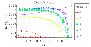
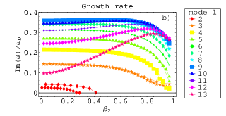
Figure 1: Stabilisation of the magnetron instability in the low-density limit. We retrieve the results of the diocotron instability. The plasma density is constant in the column, $\rho_{0}={\rm cst}$. The geometric aspect ratios are, for Fig.(a), $w=0.1$, $d_{1}=0.4$ and $d_{2}=0.5$ and, for Fig.(b), $w=0.1$, $d_{1}=0.45$ and $d_{2}=0.5$. The growth rates are normalised to the diocotron frequency, $\omega_{\rm D}$. The curves corresponding to the outgoing wave boundary conditions contain twice as much symbols as the conducting wall boundary conditions in order to distinguish them.

A simplistic approach to understand the stabilisation process is as follows. In the low-density limit, the magnetron instability reduces to the diocotron regime. Assuming a constant charge density within the plasma, unstable oscillations are generated when the surface waves at both edges of the plasma column interact in a constructive way, i.e. that oscillation have to synchronise. For high velocities within the fluid, the relative phase speed between the two waves increase, mutual synchronisation becomes difficult to reach, reducing the growth rate of the instability (Knauer, 1966).

The qualitative physical nature of the diocotron/magnetron instability can be expressed via the more familiar Kelvin-Helmholtz or two-stream instability (MacFarlane & Hay, 1950; Trivelpiece & Gould, 1959; Buneman et al., 1966). For instance, the two-stream instability is investigated in Delcroix & Bers (1994). It is found (in Cartesian geometry) that while in the long wavelength limit, the growth rate is proportional to the velocity difference between the two beams, they are reduced for sufficiently large velocity shear until the instability disappears. This stabilisation mechanism applies also to the diocotron/magnetron instability and can already occur at modest speeds, much less than the speed of light $c$.

4.2 Influence of curvature

The influence of the curvature is also studied by taking the limit of the planar diode geometry. The curvature of the plasma column is then increased to investigate the evolution of the growth rates.

The effective aspect ratio of the plasma layer is conveniently described by the parameter

$$A=\frac{R_{1}}{R_{2}-R_{1}}$$ (66)

Using the equilibrium electric field profile indicated in Sect. 2.5, in the limit of small curvature corresponding to large aspect ratio, $A\to+\infty$, the eigenvalue problem and equilibrium configuration is described by the relativistic planar diode.

We show the evolution of the growth rate in the non-relativistic limit $\beta_{2}=10^{-3}$, Fig. 2a, and in the relativistic case $\beta_{2}\approx 0.2$, Fig. 2b. The aspect ratio has a drastic influence on the growth rate. For large values of $A\gg 1$, all unstable modes are stabilised, in both non-relativistic and relativistic flows. These results agree with those found in Pétri (2007a). Note that the drift speed has only a negligible effect on the growth rate compared to the aspect ratio.

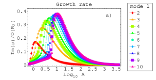
Figure 2: Effect of the cylindrical geometry on the growth rate of the instability. The growth rate are normalised to the rotation at the outer edge of the plasma column $\Omega(R_{2})$ and plotted versus the aspect ratio $A$, in logarithmic scale. In Fig.(a), the speed at the outer edge of the column is $\beta_{2}=10^{-3}$ whereas in Fig.(b), it is $\beta_{2}\approx 0.2$.

4.3 Electrosphere

Finally, we checked the results obtained for the electrosphere, with outer wall or outgoing waves. The rotation profile is chosen to mimic the rotation curve obtained in the 3D electrosphere. To study the influence of the relativistic effects, we take the same profiles as those given in Pétri (2007a, b). We remind that different analytical expressions for the radial dependence of $\Omega$ are chosen by mainly varying the gradient in differential shear as follows

$$\Omega(r)=\Omega_{*}\,(2+\tanh[\alpha\,(r-r_{0})]\,e^{-\beta\,r^{4}})$$ (67)

$\Omega_{*}$ is the neutron star spin and $r$ is normalised to the neutron star radius, $R_{*}$. The values used are listed in Table 2.

$\Omega$	$\alpha$	$\beta$	$r_{0}$
$\Omega_{2}$	1.0	$5\times 10^{-5}$	6.0
$\Omega_{3}$	0.3	$5\times 10^{-5}$	10.0

Table 2: Parameters for the rotation profiles used to mimics the azimuthal velocity of the plasma in the electrospheric disk.

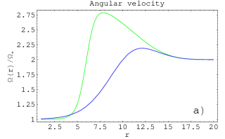
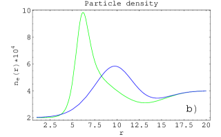
Figure 3: Two choices of differential rotation curves in the plasma column for the cylindrical pulsar electrosphere, $\Omega_{2}$ with strong shear (in green) and $\Omega_{3}$ with weak shear (in blue), Fig. (a) and the corresponding charge density, Fig.(b).

The angular velocity, and the corresponding particle density number, are shown respectively in Fig. 3a and 3b. In both cases, $\Omega$ starts from corotation with the star $\Omega=\Omega_{*}$ followed by a sharp increase around $r=6$ for $\Omega_{2}$ and a less pronounced gradient around $r=10$ for $\Omega_{3}$. Finally the rotation rate asymptotes twice the neutron star rotation speed for large radii.

The computed growth rates, normalised to the speed of the neutron star, are shown in Fig. 4, for the profile $\Omega_{2}$, Fig. 4a, and for $\Omega_{3}$, Fig. 4b.

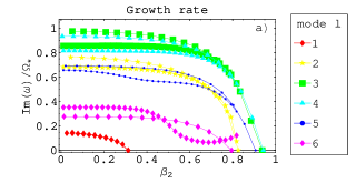
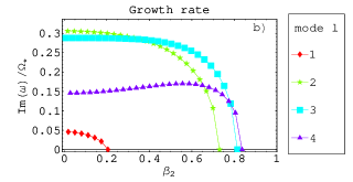
Figure 4: Evolution of the growth rates, ${\rm Im}(\omega)$, normalised to the spin of the neutron star $\Omega_{*}$, for increasing maximal speed of the column, $\beta_{2}$. For the profile $\Omega_{2}$, in Fig.(a), outer conducting wall are compared with outgoing wave boundary conditions. For the latter, the curves contain twice as much symbols as for the former boundary conditions. Note that for the mode $l=1$, the curves overlap and cannot be distinguished. For the profile $\Omega_{3}$, in Fig.(b), only the wall boundary conditions are plotted.

5 RESULTS

We demonstrated that our numerical algorithm gives accurate results in the non-relativistic cylindrical geometry for which we know an analytical expression of the eigenfrequencies. Moreover, the transition to the relativistic regime gives the same results as those shown in Pétri (2007a). In this section, we compute the eigenspectra of the relativistic magnetron instability in cylindrical coordinates, for various equilibrium density profiles, electric field, and velocity profiles. Application to pulsar’s electrosphere is also discussed.

5.1 Influence of the self-field

We study the influence of the self-electromagnetic field on the instability. When the self-field is negligible, i.e. in the low-density limit, $s_{\rm e}\ll 1$, the instability is well approximated by the diocotron regime, which means in the electric drift approximation. However, when the density of the plasma increases, $s_{\rm e}\approx 1$, it induces a strong electric field which would lead to superluminal motion in the drift approximation. Therefore, particle inertia comes into play and imposes a motion which departs significantly from the electric drift and modifies the behavior of the instability.

We considered the plasma in cylindrical geometry, confined by some external experimental electromagnetic device between the inner and outer wall. The external applied magnetic field and the density profile are specified as initial data. Thus, we deduce the velocity profile by solving the non-linear Volterra integral equation, Eq. (2.4), as explained in Sect. 2.4.

We study the influence of particle inertia in both, the non-relativistic and relativistic regime. As a starting point, we take the diocotron regime, $s_{\rm e}\ll 1$, and slowly increase the influence of the self-field parameter, $s_{\rm e}$.

Examples of growth rates are shown in Fig. 5. A non-relativistic flow ($\beta_{2}\approx 10^{-3}$) is shown in Fig. 5a whereas a mildly relativistic flow ($\beta_{2}\approx 0.19$) is shown in Fig. 5b. In both cases, increasing the self-field stabilises the magnetron regime. Close to the maximum value of the self-field parameter, the Brillouin zone above which no equilibrium configuration exists because the defocusing electric field is to strong compared to the magnetic focusing field, the instability has almost completely disappeared.

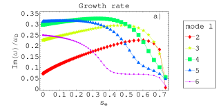
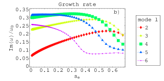
Figure 5: Influence of the self-field parameter, $s_{\rm e}$, on the magnetron instability, for a non-relativistic flow ($\beta_{2}\approx 10^{-3}$) in Fig.(a) and a relativistic flow ($\beta_{2}\approx 0.19$) in Fig.(b). The geometric aspect ratios are, $w=0.1$, $d_{1}=0.4$, and $d_{2}=0.5$, the same as those in Fig. 1a.

For completeness, the evolution of the shape of the eigenfunctions of the mode $l=5$ corresponding to the eigenvalues in Fig. 5a is shown in Fig. 6. When the stabilisation process becomes important, the real and imaginary parts of the eigenfunction possess significant negative values compared to the low self-field parameter case.

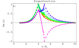
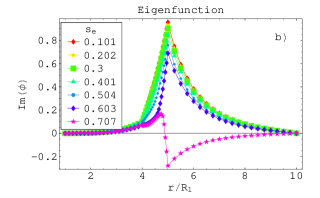
Figure 6: Real and imaginary part of the eigenfunction, respectively Fig. a and b, for the mode $l=5$ in Fig. 5a. The real part of the eigenfunction is normalised such that the maximum in absolute value is unity. The value of the self-field parameter $s_{\rm e}$ for each eigenfunction is shown in legend.

5.2 Electrosphere

The electrospheric non-neutral plasma is confined by the rotating magnetised neutron star. The most important feature is the velocity profile in the plasma column. For simplicity, here, we assume that no vacuum gaps exist between the plasma and the inner wall, $W_{1}=R_{1}$. The inner wall depicts the perfectly conducting neutron star interior. The plasma is in contact with the neutron star surface. The outer wall can be suppressed depending on the outer boundary conditions. For instance, we expect electromagnetic wave generation, leading to a net outgoing Poynting flux carrying energy to infinity. Both situations will be considered. We generalise the study presented in Pétri (2007a) by including particle inertia.

To remain fully self-consistent, we only consider an uniform applied external magnetic field. The growth rates for the rotation curve $\Omega_{2}$ for each mode $l$ are shown in Fig. 7a and those for $\Omega_{3}$ in Fig. 7b.

For $\Omega_{2}$, starting from the diocotron regime, $s_{\rm e}\ll 1$, the instability is first enhanced by the particle inertia effect, until $s_{\rm e}\approx 0.25$. Then, the growth rates begin to decrease until they vanish for the maximum allowed self-field parameter, corresponding to the last existing equilibrium configuration.

For $\Omega_{3}$, no increase is observed, the stabilisation effect proceeds as soon as $s_{\rm e}$ increases.

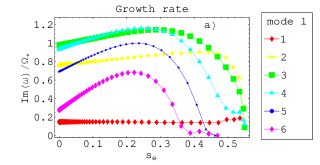
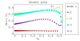
Figure 7: Evolution of the growth rates, ${\rm Im}(\omega)$, of the profiles $\Omega_{2}$, Fig.(a), and $\Omega_{3}$, Fig.(b), for increasing self-field parameter, i.e. transition from the diocotron to the magnetron regime.

Finally, we compute the evolution of the spectrum of the magnetron instability when going to the relativistic regime for a significant initial self-field parameter, $s_{\rm e}\approx 0.16$. We start with a non-relativistic rotation profile such that $\beta_{2}\ll 1$ and slowly increase $R_{2}$ (as well as $W_{1},W_{2},R_{1}$ to maintain their ratio constant) in order to approach the speed of light for the maximal rotation rate of the plasma column.

Results for the growth rates of the velocity profiles $\Omega_{2}$ and $\Omega_{3}$ are shown in Fig. 8a and b respectively.

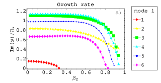
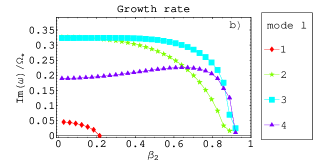
Figure 8: Evolution of the growth rates ${\rm Im}(\omega)$ of the profiles $\Omega_{2}$, Fig.(a), and $\Omega_{3}$, Fig.(b), for a significant initial self-field parameter, $s_{\rm e}\approx 0.16$.

For completeness, the evolution of the shape of the eigenfunctions of the mode $l=5$ corresponding to the eigenvalues in Fig. 8a is shown in Fig. 9. When the stabilisation process starts, the real and imaginary parts of the eigenfunction oscillate. Moreover, while these functions remain positive for small speeds, they change sign whenever the diminishing of the growth rates become significant. This behavior was already observed in the study of the influence of the self-field parameter, Sect. 5.1.

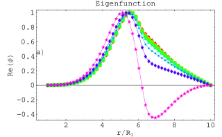
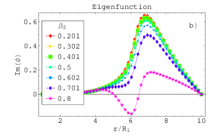
Figure 9: Real and imaginary part of the eigenfunction, respectively Fig. a and b, for the mode $l=5$ in Fig. 8a. The real part of the eigenfunction is normalised such that the maximum in absolute value is unity. The value of the maximal speed $\beta_{2}$ for each eigenfunction is shown in legend.

6 CONCLUSION

We developed a numerical code to compute the eigenspectra and eigenfunctions of the magnetron instability in cylindrical geometry, including particle inertia, as well as electromagnetic and relativistic effects, in a fully self-consistent way. It is thus possible to study the behavior of the plasma in the vicinity of the light cylinder, i.e. where the particle kinetic energy becomes comparable to the magnetic field energy density.

Unstable modes are computed for a uniform external applied magnetic field and arbitrary velocity, density and electric field profiles. The resulting equilibrium configuration is computed self-consistently, according to the cold-fluid and Maxwell equations. Application of the code to a plasma column as well as to the pulsar electrosphere have been shown. In both cases, the magnetron regime gives rise to instabilities that become less and less unstable when the self-field parameter of the flow, $s_{\rm e}$, approaches its maximum allowed value, $s_{\rm e}\lesssim s_{\rm e,max}$. Whereas the growth rates can be comparable to the rotation period of the neutron star in the non-relativistic limit, it is found that for special rotation profiles, the magnetron instability is completely suppressed in the relativistic regime, as was already the case in the diocotron limit.

However, the magnetron instability is not restricted to the electrosphere. For instance, it is believed that the pulsed radio emission emanates from the magnetic poles close to the neutron star surface. Highly relativistic and dense leptonic flows are accelerated at these polar caps, forming non-neutral plasma beams able to radiate coherent electromagnetic waves by several processes like the cyclotron maser or the free electron laser instability. We will address this problem as well as the effect of finite temperature in a forthcoming paper.