UMTG–255

The QCD spin chain $S$ matrix
Changrim Ahn , Rafael I. Nepomechie and Junji Suzuki

Beisert et al. have identified an integrable $SU(2,2)$ quantum spin chain which gives the one-loop anomalous dimensions of certain operators in large $N_{c}$ QCD. We derive a set of nonlinear integral equations (NLIEs) for this model, and compute the scattering matrix of the various (in particular, magnon) excitations.

1 Introduction

The search for integrability in QCD has a long history (see e.g. [1]-[6] and references therein). A remarkable recent development is the discovery [7] that the one-loop mixing matrix for the chiral gauge-invariant operators

$$\mathop{\rm tr}\nolimits f_{\alpha_{1}\beta_{1}}(x)\ldots f_{\alpha_{L}\beta_{L}}(x)$$ (1.1)

in the limit $N_{c}\rightarrow\infty$ is given by the integrable spin-1 antiferromagnetic XXX Hamiltonian [9, 10],

$$\Gamma={\alpha_{s}N_{c}\over 2\pi}\sum_{l=1}^{L}\left[\frac{7}{6}+\frac{1}{2}\vec{S}_{l}\cdot\vec{S}_{l+1}-\frac{1}{2}(\vec{S}_{l}\cdot\vec{S}_{l+1})^{2}\right]\,.$$ (1.2)

Here $f_{\alpha\beta}$ are the selfdual components of the Yang-Mills field strength $F_{\mu\nu}=\partial_{\mu}A_{\nu}-\partial_{\nu}A_{\mu}-ig_{YM}[A_{\mu}\,,A_{\nu}]$ (where the gauge fields $A_{\mu}(x)$ are $N_{c}\times N_{c}$ Hermitian matrices), which together with the anti-selfdual components $\bar{f}_{\dot{\alpha}\dot{\beta}}$ are defined by

$$F_{\mu\nu}=\sigma^{\ \ \ \alpha\beta}_{\mu\nu}\,f_{\alpha\beta}+\bar{\sigma}^{\ \ \ \dot{\alpha}\dot{\beta}}_{\mu\nu}\,\bar{f}_{\dot{\alpha}\dot{\beta}}\,,$$ (1.3)

where $\sigma_{\mu\nu}=i\sigma_{2}(\sigma_{\mu}\bar{\sigma}_{\nu}-\sigma_{\nu}\bar{\sigma}_{\mu})/4$, $\bar{\sigma}_{\mu\nu}=-i(\bar{\sigma}_{\mu}\sigma_{\nu}-\bar{\sigma}_{\nu}\sigma_{\mu})\sigma_{2}/4$ and $\sigma_{\mu}=(1\,,\vec{\sigma})$, $\bar{\sigma}_{\mu}=(1\,,-\vec{\sigma})$. Moreover, $\alpha_{s}=g_{YM}^{2}/4\pi$, $\alpha_{s}N_{c}$ is the ‘t Hooft coupling [1] which is assumed to be small, and $\vec{S}$ are spin-1 generators of $SU(2)$. Indeed, since $f_{\alpha\beta}$ has three independent components

$$f_{+}=f_{11}\,,\quad f_{0}=\frac{1}{\sqrt{2}}(f_{12}+f_{21})\,,\quad f_{-}=f_{22}\,,$$ (1.4)

the operators (1.1) can be identified with the Hilbert space of a periodic spin-1 quantum spin chain of length $L$. The eigenvectors and eigenvalues of $\Gamma$, i.e. the linear combinations of the operators (1.1) which are multiplicatively renormalizable and their anomalous dimensions, respectively, can therefore be obtained using the Bethe Ansatz [11, 12]. In particular, the anomalous dimensions are given by

$$\gamma={\alpha_{s}N_{c}\over 2\pi}\left(\frac{7L}{6}-\sum_{j=1}^{M_{l}}{2\over l_{j}^{2}+1}\right)\,,$$ (1.5)

where $\{l_{1}\,,\ldots\,,l_{M_{l}}\}$ are roots of the Bethe Ansatz equations (BAEs)

$$\left(l_{j}+i\over l_{j}-i\right)^{L}=\prod_{k=1\atop k\neq j}^{M_{l}}{l_{j}-l_{k}+i\over l_{j}-l_{k}-i}\,.$$ (1.6)

This result was generalized in [13] to gauge-invariant operators with derivatives

$$\mathop{\rm tr}\nolimits\,(D^{m_{1}}f)\ldots(D^{m_{L}}f)\,,$$ (1.7)

where

$$D^{m}f=D_{\alpha_{1}\dot{\alpha}_{1}}\ldots D_{\alpha_{m}\dot{\alpha}_{m}}f_{\beta\gamma}+symmetrized$$ (1.8)

(complete symmetrization in the undotted and dotted indices, respectively), and $D_{\mu}=\sigma_{\mu}^{\alpha\dot{\alpha}}D_{\alpha\dot{\alpha}}$ is the usual Yang-Mills covariant derivative. Namely, the one-loop mixing matrix for the operators (1.7) is given by an integrable $SO(4,2)=SU(2,2)$ (non-compact!) quantum spin chain Hamiltonian with spins in the representation with Dynkin labels [2,-3,0]. The anomalous dimensions are given by

$$\gamma={\alpha_{s}N_{c}\over 2\pi}\left(\frac{7L}{6}-\sum_{j=1}^{M_{l}}{2\over l_{j}^{2}+1}+\sum_{j=1}^{M_{u}}{3\over u_{j}^{2}+9/4}\right)\,,$$ (1.9)

where the BAEs are now given by

$$\left(l_{j}+i\over l_{j}-i\right)^{L} = \prod_{k=1\atop k\neq j}^{M_{l}}{l_{j}-l_{k}+i\over l_{j}-l_{k}-i}\prod_{k=1}^{M_{u}}{l_{j}-u_{k}-i/2\over l_{j}-u_{k}+i/2}\,,$$

$$\left(u_{j}-3i/2\over u_{j}+3i/2\right)^{L} = \prod_{k=1\atop k\neq j}^{M_{u}}{u_{j}-u_{k}+i\over u_{j}-u_{k}-i}\prod_{k=1}^{M_{l}}{u_{j}-l_{k}-i/2\over u_{j}-l_{k}+i/2}\prod_{k=1}^{M_{r}}{u_{j}-r_{k}-i/2\over u_{j}-r_{k}+i/2}\,,$$ (1.10)

$$1 = \prod_{k=1\atop k\neq j}^{M_{r}}{r_{j}-r_{k}+i\over r_{j}-r_{k}-i}\prod_{k=1}^{M_{u}}{r_{j}-u_{k}-i/2\over r_{j}-u_{k}+i/2}\,.$$

As noted by Beisert et al., a $u$-root corresponds to adding a covariant derivative $D_{1{\dot{1}}}$; and an $l$-root and an $r$-root flip a left-Lorentz-spin $1\to 2$ and a right-spin ${\dot{1}}\to{\dot{2}}$, respectively. The scaling dimensions and $SU(2)_{L}\times SU(2)_{R}$ quantum numbers are given by

$$D=2L+M_{u}\,,\quad S_{1}=L+{1\over 2}M_{u}-M_{l}\,,\quad S_{2}={1\over 2}M_{u}-M_{r}\,,$$ (1.11)

respectively.

As noted in [13], the BAEs (1.10) can be obtained from those of the “beast” form of ${\cal N}=4$ SYM [14] by truncating the supergroup $SU(2,2|4)$ down to the Bosonic subgroup $SU(2,2)$. Much attention has been focused on the $S$ matrix of ${\cal N}=4$ SYM and of the corresponding string theory (see e.g. [16] ).

For the pure spin-1 problem (1.5), (1.6), the ground state for large $L$ is described by a “sea” of approximate “2-strings” of $l$-roots [11, 12] (in contrast to the case of the spin-1/2 antiferromagnetic XXX chain, for which the ground state is described by a sea of real roots). The excitations consist of “spinons” (roughly speaking, “holes” in the sea) which carry RSOS [17] quantum numbers. The spinon-spinon $S$ matrix was found by indirect methods in [18, 19], correcting the result obtained in [11] using the string hypothesis. A nonlinear integral equation (NLIE) [20, 21] has been obtained for this model [22]-[24], which does not rely on the string hypothesis and provides a more direct way to compute the $S$ matrix [25]. The NLIE of the $SU(2)$ sector of ${\cal N}=4$ SYM has been studied in [26].

For the general case (1.9), (1.10), the ground state is still a sea of approximate 2-strings of $l$-roots, since the $u$-roots contribute positively to the energy (and the $r$-roots do not contribute at all). Hence, there are again spinon excitations corresponding to holes in the sea. However, there are now also “magnon” excitations, corresponding to $u$-roots [13].

Our main objective here is to further investigate these magnon excitations, and in particular, to compute the magnon-magnon $S$ matrix. Owing to the nontrivial nature of the ground state, this $S$ matrix (like the spinon-spinon $S$ matrix) must be computed with care: using the string hypothesis as in [11] gives an incorrect result. To this end, we first derive in Sec. 2 a set of NLIEs for the model. Although we do not invoke the string hypothesis, we do make a certain analyticity assumption in order to describe the $u$-roots. For simplicity, we restrict to real $u$-roots, and we do not consider $r$-roots. We then use these NLIEs to determine the energy and momentum of the excitations (Sec. 3), and their $S$ matrices (Sec. 4). We end in Sec. 5 with a brief discussion of our results.

2 Nonlinear integral equations

We restrict our attention to the case without $r$-roots ($M_{r}=0$), for which the BAEs (1.10) reduce to

$$\left(l_{j}+i\over l_{j}-i\right)^{L} = \prod_{k=1\atop k\neq j}^{M_{l}}{l_{j}-l_{k}+i\over l_{j}-l_{k}-i}\prod_{k=1}^{M_{u}}{l_{j}-u_{k}-i/2\over l_{j}-u_{k}+i/2}\,,$$ (2.1)

$$\left(u_{j}-3i/2\over u_{j}+3i/2\right)^{L} = \prod_{k=1\atop k\neq j}^{M_{u}}{u_{j}-u_{k}+i\over u_{j}-u_{k}-i}\prod_{k=1}^{M_{l}}{u_{j}-l_{k}-i/2\over u_{j}-l_{k}+i/2}\,.$$ (2.2)

We now proceed in turn to recast these two sets of BAEs in the form of NLIEs.

2.1 The first set of BAEs (2.1) and an auxiliary inhomogeneous mixed spin chain

An important hint on how to analyze the first set of BAEs (2.1) comes from rewriting it in the obviously equivalent form

$$\left(l_{j}+i\over l_{j}-i\right)^{L}\prod_{k=1}^{M_{u}}{l_{j}-u_{k}+i/2\over l_{j}-u_{k}-i/2}=\prod_{k=1\atop k\neq j}^{M_{l}}{l_{j}-l_{k}+i\over l_{j}-l_{k}-i}\,.$$ (2.3)

We recognize these as the BAEs for an inhomogeneous “mixed” spin chain which has two types of spins: spin-1 and spin-1/2, with $L$ of the former and $M_{u}$ of the latter. (See, e.g., [27].) Moreover, the latter have associated “inhomogeneities” $iu_{k}$, $k=1,\ldots,M_{u}$.

We therefore consider an auxiliary integrable inhomogeneous mixed quantum spin chain, where the number of spin-1 and spin-1/2 “quantum” spaces are given respectively by $L$ and $M_{u}$; and with spectral parameter inhomogeneities $iu_{k}$ only for the spin-1/2 spins. This chain has two relevant transfer matrices $T_{1}(x)\,,T_{2}(x)$, corresponding to “auxiliary” spaces which are spin-1/2 (2-dimensional) and spin-1 (3-dimensional), respectively.

We find by standard methods that the eigenvalues of these transfer matrices (which we denote by the same notation) are given by

$$T_{1}(x) = \psi(x-i/2)\phi(x-i)\frac{Q(x+i)}{Q(x)}+\psi(x+i/2)\phi(x+i)\frac{Q(x-i)}{Q(x)}\,,$$ (2.4)

$$T_{2}(x) = \psi(x)\psi(x-i)\phi(x-i/2)\phi(x-3i/2)\frac{Q(x+3i/2)}{Q(x-i/2)}$$ (2.5)

$$+ \psi(x)^{2}\phi(x-i/2)\phi(x+i/2)\frac{Q(x+3i/2)Q(x-3i/2)}{Q(x+i/2)Q(x-i/2)}$$

$$+ \psi(x)\psi(x+i)\phi(x+i/2)\phi(x+3i/2)\frac{Q(x-3i/2)}{Q(x+i/2)}$$

$$:= \lambda_{1}(x)+\lambda_{2}(x)+\lambda_{3}(x)\,,$$

where

$$\phi(x)=x^{L}\,,\quad\psi(x)=\prod_{j=1}^{M_{u}}(x-u_{j})\,,\quad Q(x)=\prod_{j=1}^{M_{l}}(x-l_{j})\,.$$ (2.6)

Indeed, the BAEs obtained by demanding that $T_{1}(x)$ be analytic at $x=l_{j}$ (zeros of $Q(x)$) coincide with (2.1).

Evidently $T_{2}(x)$ has the common factor $\psi(x)$, which has “trivial” zeros. We therefore introduce the renormalized $T_{2}$,

$$T_{2}(x)=\psi(x)\,T^{(r)}_{2}(x)\,.$$

We note that

$$S_{1}=S^{z}_{1}=L+\frac{M_{u}}{2}-M_{l}\,,$$ (2.7)

and we recall that the “energy” is given by (1.9).

2.1.1 Physical degrees of freedom

For simplicity, we restrict $u_{k}$ to be real, and $M_{u}=1,2$. For now, we also assume that $u_{k}$ are given by hand, with (in the case $M_{u}=2$) $u_{1}=-u_{2}$. We shall discuss how they should be determined later in Sec. 2.2.

Numerical studies for small values of $L$ suggest that:

• For $M_{u}=1$, the lowest energy state in the $S^{z}_{1}=1/2$ sector is characterized by a single zero ($\vartheta_{\alpha}$) of $T_{1}(x)$, and a single zero ($\theta_{h}$) of $T^{(r)}_{2}(x)$. Both of these zeros lie on the real axis.

• For $M_{u}=2$, the lowest energy state is in the $S^{z}_{1}=0$ sector. In the “physical strip” ($-1/2\leq\Im m\,x\leq 1/2$), $T_{1}(x)$ and $T^{(r)}_{2}(x)$ are free from zeros.

• For $M_{u}=2$, the second-lowest energy state is in the $S^{z}_{1}=1$ sector. It is characterized by two zeros ($\vartheta_{\alpha}$) of $T_{1}(x)$ and two zeros ($\theta_{h}$) of $T^{(r)}_{2}(x)$. These zeros lie on the real axis.

These observations suggest that three sets of real parameters are needed to describe the physical degrees of freedom: $u_{j}\,,\vartheta_{\alpha}\,,\theta_{h}$. The first and third parameters correspond to magnon and spinon rapidities, respectively. The second parameter, which seems to correspond to excitation of the RSOS degree of freedom, is not discussed in [13].

2.1.2 The auxiliary functions and algebraic relations among them

As in previous studies [22, 24], we introduce a pair of auxiliary functions

$$\mathfrak{b}_{1}(x):=\frac{\lambda_{1}(x)+\lambda_{2}(x)}{\lambda_{3}(x)}\qquad\Im m\,x\geq 0\,,\qquad\bar{\mathfrak{b}}_{1}(x):=\frac{\lambda_{2}(x)+\lambda_{3}(x)}{\lambda_{1}(x)}\qquad\Im m\,x\leq 0\,,$$ (2.8)

where $\lambda_{i}(x)$ are defined in (2.5). They are free from zeros and poles near the real axis. This will be apparent from the following representations,

$$\mathfrak{b}_{1}(x) = \frac{\phi_{-1/2}}{\psi_{1}\phi_{3/2}\phi_{1/2}}\frac{Q(x+3i/2)}{Q(x-3i/2)}T_{1}(x-i/2)\,,$$

$$\bar{\mathfrak{b}}_{1}(x) = \frac{\phi_{1/2}}{\psi_{-1}\phi_{-3/2}\phi_{-1/2}}\frac{Q(x-3i/2)}{Q(x+3i/2)}T_{1}(x+i/2)\,.$$ (2.9)

We have introduced here the abbreviated notation $\phi_{a}:=\phi(x+ia)$, and similarly for $\psi$, which we shall use throughout this part of the paper.

At this stage, there seems to be no reason why the two auxiliary functions should be introduced in the corresponding half planes. This will become clear at a later stage.

The upper-case functions are also introduced: $\mathfrak{B}_{1}(x)=1+\mathfrak{b}_{1}(x)$, $\bar{\mathfrak{B}}_{1}(x)=1+\bar{\mathfrak{b}}_{1}(x)$, and the following relations are also useful:

$$T^{(r)}_{2}(x) = \psi_{1}\phi_{1/2}\phi_{3/2}\frac{Q(x-3i/2)}{Q(x+i/2)}\mathfrak{B}_{1}(x)$$ (2.10)

$$= \psi_{-1}\phi_{-1/2}\phi_{-3/2}\frac{Q(x+3i/2)}{Q(x-i/2)}\bar{\mathfrak{B}}_{1}(x)\,.$$ (2.11)

Apparently $\mathfrak{B}_{1}(x)$ vanishes at $x=\theta_{h}$, but it remains nonzero at $x=u_{j}$.

We now define the most important functions,

$$\mathfrak{b}(x) =\mathfrak{b}_{1}(x+i\epsilon)\,, \mathfrak{B}(x) =\mathfrak{B}_{1}(x+i\epsilon) \Im m\,x\geq 0\,,$$ (2.12)

$$\bar{\mathfrak{b}}(x) =\bar{\mathfrak{b}}_{1}(x-i\epsilon)\,, \bar{\mathfrak{B}}(x) =\bar{\mathfrak{B}}_{1}(x-i\epsilon) \Im m\,x\leq 0\,.$$ (2.13)

Here $\epsilon$ denotes a positive quantity which is slightly larger than the deviation of the 2-strings from their “perfect” positions. Therefore $\mathfrak{B}$ would possess zeros (due to the factor $Q(x+i/2)$ in (2.10)) slightly below the real axis if it were defined in the whole complex plane. The function $\mathfrak{B}$ is, however, defined only in the upper half plane (including the real axis).

Another auxiliary function originates from the so-called fusion formula that relates the two transfer matrices,

$$T_{1}(x-i/2)\,T_{1}(x+i/2)=\psi_{1}\psi_{-1}\phi_{3/2}\phi_{-3/2}+\psi_{0}T^{(r)}_{2}(x)\,,$$ (2.14)

which can be verified using (2.4) and (2.5). For later convenience, we renormalize $T_{1}(x)=\prod_{\alpha=1}^{N_{\vartheta}}\tanh\frac{\pi}{2}(x-\vartheta_{\alpha})\,T_{1}^{(r)}(x)$, and rewrite the above in the form

$$T_{1}^{(r)}(x-i/2)\,T_{1}^{(r)}(x+i/2) = \psi_{1}\psi_{-1}\phi_{3/2}\phi_{-3/2}+\psi_{0}T^{(r)}_{2}(x)$$ (2.15)

$$= \psi_{1}\psi_{-1}\phi_{3/2}\phi_{-3/2}\,Y(x)\,,$$

where we have defined the auxiliary functions

$$y(x):=\frac{\psi_{0}}{\psi_{1}\psi_{-1}\phi_{3/2}\phi_{-3/2}}T^{(r)}_{2}(x)\,,\qquad Y(x):=1+y(x)\,.$$ (2.16)

Since $y$ possesses zeros on the real axis due to $u_{j}$ and $\theta_{h}$, we also define a renormalized function $y^{(r)}$

$$y(x)=\prod_{j=1}^{M_{u}}\tanh\frac{\pi}{2}(x-u_{j})\prod_{h=1}^{N_{h}}\tanh\frac{\pi}{2}(x-\theta_{h})\,y^{(r)}(x)\,,$$ (2.17)

which obeys the functional relation

$$y^{(r)}(x-i/2)\,y^{(r)}(x+i/2)=\mathfrak{B}_{1}(x+i/2)\,\bar{\mathfrak{B}}_{1}(x-i/2)\,,$$ (2.18)

as follows from (2.10) and (2.11).

2.1.3 Derivation of NLIE

The derivation of the NLIE can be most easily done in Fourier space. For a smooth function $f(x)$, we define

$$\hat{f}[k]=\frac{1}{2\pi}\int_{-\infty}^{\infty}{\rm e}^{ikx}f(x)\,dx\,,\qquad f(x)=\int_{-\infty}^{\infty}{\rm e}^{-ikx}\hat{f}[k]\,dk.$$ (2.19)

We also introduce the special notation

$$\widehat{dlf}[k]=\frac{1}{2\pi}\int_{-\infty}^{\infty}{\rm e}^{ikx}\left[\ln f(x)\right]^{\prime}dx$$ (2.20)

which will be frequently used below.

It is convenient to introduce “shifted” $Q$ functions,

$$q_{1}(x):=Q(x-i/2-i\epsilon)\,,\qquad q_{2}(x):=Q(x+i/2+i\epsilon)\,.$$ (2.21)

By definition, $q_{1}$ is Analytic and NonZero (ANZ) for $\Im m\,x\leq 0$, while $q_{2}$ is ANZ for $\Im m\,x\geq 0$. We therefore have by Cauchy’s theorem the important property

$$\widehat{dlq}_{2}[k>0]=\widehat{dlq}_{1}[k<0]=0\,.$$ (2.22)

Similarly,

$$\widehat{dl\psi}_{a}[k>0]=\widehat{dl\phi}_{a}[k>0]=0\mbox{ for }a>0\,,\quad\widehat{dl\psi}_{a}[k<0]=\widehat{dl\phi}_{a}[k<0]=0\mbox{ for }a<0\,.$$ (2.23)

We slightly shift the arguments in (2.10), (2.11)

$$T^{(r)}_{2}(x+i\epsilon) = \psi_{1+\epsilon}\phi_{1/2+\epsilon}\phi_{3/2+\epsilon}\frac{q_{1}(x-i+2i\epsilon)}{q_{2}(x)}\mathfrak{B}(x)\,,$$ (2.24)

$$T^{(r)}_{2}(x-i\epsilon) = \psi_{-1-\epsilon}\phi_{-1/2-\epsilon}\phi_{-3/2-\epsilon}\frac{q_{2}(x+i-2i\epsilon)}{q_{1}(x)}\bar{\mathfrak{B}}(x)\,.$$ (2.25)

We then use the result

$$\frac{1}{2\pi}\int_{C_{\epsilon}}{\rm e}^{ikx}\left[\ln T_{2}^{(r)}(x)\right]^{\prime}dx=i\sum_{h}{\rm e}^{ik\theta_{h}}\,,$$ (2.26)

where we choose the contour $C_{\epsilon}$ as in Figure 1,

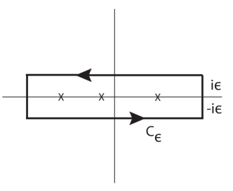
Figure 1: Integration contour

and we obtain the following

$$\widehat{dlq}_{1}[k>0] = \frac{\widehat{dl\psi}_{-1-\epsilon}+\widehat{dl\phi}_{-3/2-\epsilon}+\widehat{dl\phi}_{-1/2-\epsilon}}{1+{\rm e}^{-k}}+\frac{\widehat{dl\bar{\mathfrak{B}}}[k]-{\rm e}^{-2k\epsilon}\widehat{dl\mathfrak{B}}[k]}{1+{\rm e}^{-k}}$$ (2.27)

$$-i\sum_{h}\frac{{\rm e}^{ik\theta_{h}-k\epsilon}}{1+{\rm e}^{-k}}\,,$$

$$\widehat{dlq}_{2}[k<0] = \frac{\widehat{dl\psi}_{1+\epsilon}+\widehat{dl\phi}_{3/2+\epsilon}+\widehat{dl\phi}_{1/2+\epsilon}}{1+{\rm e}^{k}}+\frac{\widehat{dl\mathfrak{B}}[k]-{\rm e}^{2k\epsilon}\widehat{dl\bar{\mathfrak{B}}}[k]}{1+{\rm e}^{k}}$$ (2.28)

$$+i\sum_{h}\frac{{\rm e}^{ik\theta_{h}+k\epsilon}}{1+{\rm e}^{k}}\,.$$

In addition, from (2.15), one derives

$$\widehat{dlT}_{1}[k]=\frac{\widehat{dl\psi}_{\mp 1}+\widehat{dl\phi}_{\mp 3/2}}{{\rm e}^{k/2}+{\rm e}^{-k/2}}+\frac{\widehat{dlY}}{{\rm e}^{k/2}+{\rm e}^{-k/2}}+i\sum_{\alpha}\frac{{\rm e}^{ik\vartheta_{\alpha}+k/2}}{{\rm e}^{k/2}+{\rm e}^{-k/2}}\,,$$ (2.29)

where $-(k>0)$ and $+(k<0)$.

We shift the arguments in (2.9)

$$\mathfrak{b}(x) = \frac{\phi_{-1/2+\epsilon}}{\psi_{1+\epsilon}\phi_{3/2+\epsilon}\phi_{1/2+\epsilon}}\frac{q_{2}(x+i)}{q_{1}(x-i+2i\epsilon)}T_{1}(x-i/2+i\epsilon)\,,$$

$$\bar{\mathfrak{b}}(x) = \frac{\phi_{1/2-\epsilon}}{\psi_{-1-\epsilon}\phi_{-3/2-\epsilon}\phi_{-1/2-\epsilon}}\frac{q_{1}(x-i)}{q_{2}(x+i-2i\epsilon)}T_{1}(x+i/2-i\epsilon)\,,$$ (2.30)

and then take the Fourier transformation. The substitution of (2.27 ), (2.28 ) and (2.29) into the resultant transformation then leads to the NLIE in Fourier space,

$$\widehat{dlb}[k>0] = \frac{\widehat{dl\phi}_{-1/2+\epsilon}}{1+{\rm e}^{-k}}+i\sum_{h}\frac{{\rm e}^{ik\theta_{h}+\epsilon k}}{1+{\rm e}^{k}}+i\sum_{\alpha}\frac{{\rm e}^{ik\vartheta_{\alpha}+\epsilon k}}{{\rm e}^{k/2}+{\rm e}^{-k/2}}$$ (2.31)

$$+ \frac{{\rm e}^{-k/2+\epsilon k}}{{\rm e}^{k/2}+{\rm e}^{-k/2}}\widehat{dlY}[k]+\frac{1}{{\rm e}^{k}+1}(\widehat{dl\mathfrak{B}}[k]-{\rm e}^{2k\epsilon}\widehat{dl\bar{\mathfrak{B}}}[k])\,,$$

$$\widehat{dlb}[k<0] = -\frac{\widehat{dl\phi}_{1/2+\epsilon}}{1+{\rm e}^{k}}+i\sum_{h}\frac{{\rm e}^{ik\theta_{h}+\epsilon k}}{1+{\rm e}^{-k}}+i\sum_{\alpha}\frac{{\rm e}^{ik\vartheta_{\alpha}+\epsilon k}}{{\rm e}^{k/2}+{\rm e}^{-k/2}}$$ (2.32)

$$+ \frac{{\rm e}^{-k/2+\epsilon k}}{{\rm e}^{k/2}+{\rm e}^{-k/2}}\widehat{dlY}[k]+\frac{1}{{\rm e}^{-k}+1}(\widehat{dl\mathfrak{B}}[k]-{\rm e}^{2k\epsilon}\widehat{dl\bar{\mathfrak{B}}}[k])\,.$$

Interestingly, although a contribution from the inhomogeneities ($\psi$) appeared during the calculation, it cancelled in the final form. An equation for $y$ is immediately derived from (2.18),

$$\widehat{dly}[k] = i\sum_{h}\frac{{\rm e}^{ik\theta_{h}}}{1+{\rm e}^{-k}}+i\sum_{j}\frac{{\rm e}^{iku_{j}}}{1+{\rm e}^{-k}}$$ (2.33)

$$+ \frac{{\rm e}^{k(1/2-\epsilon)}}{{\rm e}^{k/2}+{\rm e}^{-k/2}}\widehat{dl\mathfrak{B}}[k]+\frac{{\rm e}^{-k(1/2-\epsilon)}}{{\rm e}^{k/2}+{\rm e}^{-k/2}}\widehat{dl\bar{\mathfrak{B}}}[k]\,.$$

In the original coordinate space, the resultant equations read

$$\ln\mathfrak{b}(x) = iD_{b}(x+i\epsilon)+\int_{-\infty}^{\infty}G_{s}(x-x^{\prime})\ln\mathfrak{B}(x^{\prime})\,dx^{\prime}-\int_{-\infty}^{\infty}G_{s}(x-x^{\prime}+2i\epsilon)\ln\bar{\mathfrak{B}}(x^{\prime})\,dx^{\prime}$$ (2.34)

$$+ \int_{-\infty}^{\infty}K(x-x^{\prime}-i/2+i\epsilon)\ln Y(x^{\prime})\,dx^{\prime}\,,$$

$$\ln y(x) = iD_{y}(x)+\int_{-\infty}^{\infty}K(x-x^{\prime}+i/2-i\epsilon)\ln\mathfrak{B}(x^{\prime})\,dx^{\prime}$$ (2.35)

$$+ \int_{-\infty}^{\infty}K(x-x^{\prime}-i/2+i\epsilon)\ln\bar{\mathfrak{B}}(x^{\prime})\,dx^{\prime}\,,$$

where

$$G_{s}(x)=\frac{1}{2\pi}\int_{-\infty}^{\infty}\frac{{\rm e}^{-ikx}}{1+{\rm e}^{|k|}}dk\,,\qquad K(x)=\frac{1}{2\pi}\int_{-\infty}^{\infty}\frac{1}{2\cosh(k/2)}{\rm e}^{-ikx}\,dk=\frac{1}{2\cosh(\pi x)}\,.$$ (2.36)

The source term in (2.34) consists of the bulk (“driving”) contribution and the contribution from the hole excitations,

$$D_{b}(x)=D^{(b)}_{\rm bulk}(x)+D^{(b)}_{\rm hole}(x)-\frac{\pi}{2}N_{h}\,,$$ (2.37)

where

$$D^{(b)}_{\rm bulk}(x)=L\chi_{K}(x)\,,\qquad D^{(b)}_{\rm hole}(x)=\sum_{\alpha=1}^{N_{\vartheta}}\chi_{K}(x-\vartheta_{\alpha})+\sum_{h=1}^{N_{h}}\chi(x-\theta_{h})\,,$$ (2.38)

and

$$\chi^{\prime}_{K}(x)=2\pi K(x)\,,\qquad\chi^{\prime}(x)=2\pi G_{s}(x)\,.$$ (2.39)

In particular, on suitable domains (containing the positive real axis),

$$\chi_{K}(x)=\frac{1}{i}\ln\tanh(\pi(x-i/2)/2)=i\ln\frac{\sinh(\pi(x+i/2)/2)}{\sinh(\pi(x-i/2)/2)}+\frac{\pi}{2}=\arctan(\sinh(\pi x))-\frac{\pi}{2}\,,$$

where $\chi_{K}(0)\equiv-\pi/2$, and also $\chi(0)\equiv 0$. The source term in (2.35) is given by

$$D_{y}(x) = \sum_{h=1}^{N_{h}}\chi_{K}(x-\theta_{h}+i/2)+\sum_{j=1}^{M_{u}}\chi_{K}(x-u_{j}+i/2)\,.$$ (2.41)

The parameters $(u_{j},\vartheta_{\alpha},\theta_{h})$ must actually be determined again by NLIEs. Indeed, (2.10) implies that the hole rapidities $\theta_{h}$ are determined by

$$\mathfrak{b}(\theta_{h}-i\epsilon)=\mathfrak{b}_{1}(\theta_{h})=-1\,,$$ (2.42)

which also leads to the determination of the spinon-spinon and spinon-magnon scattering matrices, as discussed in Sec. 4.

In order to fix the parameters $\vartheta_{\alpha}$, we need another NLIE. We consider the most natural auxiliary function ${\mathfrak{a}}(x)$, defined by

$${\mathfrak{a}}(x):=\frac{\lambda_{1}(x+i/2)}{\lambda_{2}(x+i/2)}=\frac{\lambda_{2}(x-i/2)}{\lambda_{3}(x-i/2)}\,,$$ (2.43)

where again $\lambda_{i}(x)$ are defined in (2.5). From (2.4) we have

$$T_{1}(x)=\psi_{1/2}\phi_{1}\frac{Q(x-i)}{Q(x)}\left[1+{\mathfrak{a}}(x)\right]\,.$$ (2.44)

Hence, the zeros of $T_{1}$ on the real axis $\vartheta_{\alpha}$ satisfy

$$\mathfrak{a}(\vartheta_{\alpha})=-1\,.$$ (2.45)

We omit the derivation of the NLIE for $\mathfrak{a}(x)$ for $|\Im m\,x|<1/2$, which is similar to the one for the trigonometric and homogeneous case considered in [24]. The result is

$$\ln\mathfrak{a}(x)=iD_{a}(x)+\int_{-\infty}^{\infty}K(x-x^{\prime}-i\epsilon)\ln\mathfrak{B}(x^{\prime})\,dx^{\prime}-\int_{-\infty}^{\infty}K(x-x^{\prime}+i\epsilon)\ln\bar{\mathfrak{B}}(x^{\prime})\,dx^{\prime}\,,$$ (2.46)

where the source term is given by

$$D_{a}(x)=\sum_{h=1}^{N_{h}}\chi_{K}(x-\theta_{h})+\sum_{j=1}^{M_{u}}\chi_{K}(x-u_{j})\,.$$ (2.47)

2.2 The second set of BAEs (2.2)

We finally consider an equation to fix the magnon rapidities $u_{j}$. For this purpose, we propose an expression for the transfer matrix eigenvalues similar to the one for the $su(3)$ spin chain,

$$\tau(x) = \phi(x-i)\frac{Q(x+i)}{Q(x)}+\phi(x+i)\frac{\psi(x+i/2)}{\psi(x-i/2)}\frac{Q(x-i)}{Q(x)}+\phi(x-2i)\frac{\psi(x-3i/2)}{\psi(x-i/2)}$$ (2.48)

$$:= \tau_{1}(x)+\tau_{2}(x)+\tau_{3}(x)\,.$$

Indeed, demanding analyticity of $\tau(x)$ at $x=l_{j}$ (zeros of $Q(x)$) gives the BAEs (2.1), while demanding analyticity at $x=u_{j}+i/2$ (zeros of $\psi(x-i/2)$) gives the BAEs (2.2).

Because of its similarity to the $su(3)$ transfer matrix eigenvalue, we shall assume that $\tau(x)$ is ANZ in the strip $-1/2\leq\Im m\,x\leq 1/2$, which is indeed the analyticity property for the $su(3)$ case. This assumption can in principle be checked numerically for small values of $L$. However, we have so far not succeeded to do so, due to the difficulty of finding numerical solutions of the BAEs (2.1), (2.2).

This assumption leads to a simple determination of $u_{j}$ as follows. Let us consider an auxiliary function introduced in studies of the supersymmetric $tJ$ model [28] and the $su(3)$ vertex model [29],

$$\mathfrak{c}(x):=\frac{\tau_{3}(x+i/2)}{\tau_{1}(x+i/2)+\tau_{2}(x+i/2)}\,.$$ (2.49)

It is easy to check that this can be rewritten in terms of $T_{1}(x)$ in (2.4),

$$\mathfrak{c}(x)=\frac{\psi(x-i)\phi(x-3i/2)}{T_{1}(x+i/2)}\,.$$ (2.50)

We then have

$$\mathfrak{c}(u_{j})=-1\,,$$ (2.51)

which follows from

$$\mathfrak{C}(x)=1+\mathfrak{c}(x)=\frac{\tau(x+i/2)}{\tau_{1}(x+i/2)+\tau_{2}(x+i/2)}=\frac{\tau(x+i/2)\,\psi(x)}{T_{1}(x+i/2)}\,.$$ (2.52)

From our above assumption on the analyticity of $\tau(x)$, the zeros of $\mathfrak{C}(x)$ near the real axis are determined by those of $\psi(x)$, namely $u_{j}$.

The NLIE for $\mathfrak{c}$ is obtained from the knowledge of $T_{1}$. The result is

$$\ln\mathfrak{c}(x)=iD_{c}(x)-\int_{-\infty}^{\infty}K(x-x^{\prime}+i/2)\ln Y(x^{\prime})\,dx^{\prime}\,,$$ (2.53)

where the source term is given by

$$D_{c}(x) = L\chi_{2}(x)+\sum_{j=1}^{M_{u}}\chi_{3/2}(x-u_{j})+\sum_{\alpha=1}^{N_{\vartheta}}\chi_{K}(x-\vartheta_{\alpha})-\frac{\pi}{2}(L+M_{u})\,,$$ (2.54)

and

$$\chi_{a}^{\prime}(x)=2\pi K_{a}(x)\,,\quad K_{a}(x)=\frac{1}{2\pi}\int_{-\infty}^{\infty}\frac{{\rm e}^{-a|k|-ikx}}{2\cosh\frac{k}{2}}dk\,,\quad\chi_{a}(0)\equiv 0\,,\quad a=3/2\,,2\,.$$ (2.55)

2.3 Counting functions and counting equations

So-called counting equations relating the various types of Bethe roots and excitations in a given state can be derived from corresponding counting functions associated with the auxiliary functions . These counting equations help determine the spins of the excitations.

We continue to restrict to the case of real $u$-roots and no $r$-roots. As in previous studies [21, 24, 25], it is convenient to classify $l$-roots according to their imaginary parts as follows:

2-strings

: pairs of complex-conjugate roots $x_{j}\pm iy_{j}$ with $0<y_{j}-1/2<\!\!<1$, $j=1,\ldots,M_{2}/2$

real roots

: $\Im m\,l_{j}=0$, $j=1,\ldots,M_{real}$

inner roots

: $|\Im m\,l_{j}|<1/2$, $j=1,\ldots,M_{I}$

close roots

: $1/2<|\Im m\,l_{j}|<3/2$, $j=1,\ldots,M_{C}$

wide roots

: $|\Im m\,l_{j}|>3/2$, $j=1,\ldots,M_{W}$

Hence,

$$M_{l}=M_{real}+M_{2}+M_{I}+M_{C}+M_{W}\,.$$ (2.56)

It is also convenient to introduce the functions

$$\theta_{\mp}(x,\alpha)=\frac{1}{i}\ln\left(\mp\frac{x-i\alpha}{x+i\alpha}\right)\,.$$ (2.57)

Note that $\theta_{-}(x,\alpha)=2\arctan(x/\alpha)$ has branch points in the complex $x$ plane at $x=\pm i\alpha$; following [21], we choose the corresponding branch cuts to be parallel to the real axis, extending from $i\alpha$ to $+\infty+i\alpha$, and from $-\infty-i\alpha$ to $-i\alpha$. This function has a discontinuity of $-2\pi$ when crossing the cuts from below. Similarly, we add to $\theta_{+}(x,\alpha)$ a $2\pi$-discontinuity at $x=0$ so that it is a continuous function of $x$.

We define the counting function $z_{\mathfrak{a}}(x)$ associated with the auxiliary function $\mathfrak{a}(x)$ (2.43) by

$$z_{\mathfrak{a}}(x)=\frac{1}{i}{\rm Log}\,\mathfrak{a}(x)=L\theta_{-}(x,1)-\sum_{j=1}^{M_{l}}\theta_{-}(x-l_{j},1)+\sum_{j=1}^{M_{u}}\theta_{+}(x-u_{j},1/2)\,.$$ (2.58)

We have verified numerically for various states that $z_{\mathfrak{a}}(x)$ is a continuous increasing function of $x$. This function “counts” zeros of $T_{1}(x)$ and real $l$-roots. That is,

$$z_{\mathfrak{a}}(x_{j})=2\pi I_{j}^{\mathfrak{a}}\,,$$ (2.59)

where $I_{j}^{\mathfrak{a}}$ is integer ($S_{1}-S_{2}$ odd) or half-odd integer ($S_{1}-S_{2}$ even) if $x_{j}$ is a zero of $T_{1}(x)$ or a real $l$-root. Defining integers or half-odd integers $I_{max}^{\mathfrak{a}}$ and $I_{min}^{\mathfrak{a}}$ by

$$z_{\mathfrak{a}}(+\infty) = 2\pi\left(I_{max}^{\mathfrak{a}}+\frac{1}{2}\right)\,,$$

$$z_{\mathfrak{a}}(-\infty) = 2\pi\left(I_{min}^{\mathfrak{a}}-\frac{1}{2}\right)\,,$$ (2.60)

it follows from (2.58) and (2.59), respectively, that

$$I_{max}^{\mathfrak{a}}-I_{min}^{\mathfrak{a}}+1 = S_{1}+S_{2}+M_{b}$$ (2.61)

$$= N_{\vartheta}+M_{real}\,,$$

where $M_{b}$ is the number of $l$-roots $l_{j}$ with $|\Im m\,l_{j}|>1$. We therefore arrive at the first counting equation

$$N_{\vartheta}=S_{1}+S_{2}+M_{b}-M_{real}\,.$$ (2.62)

Similarly, we define the counting function $z_{\mathfrak{b}}(x)$ associated with the auxiliary function $\mathfrak{b}_{1}(x)$ (2.8) by

$$z_{\mathfrak{b}}(x) = \Re e\,\frac{1}{i}{\rm Log}\,\mathfrak{b}_{1}(x)=\Re e\,\Big{\{}\frac{1}{i}\ln\left[1+\frac{1}{\mathfrak{a}(x-i/2)}\right]+\sum_{j=1}^{M_{u}}\theta_{+}(x-u_{j},1)$$ (2.63)

$$+ L\left[\theta_{-}(x,1/2)+\theta_{-}(x,3/2)\right]-\sum_{j=1}^{M_{l}}\left[\theta_{-}(x-l_{j},1/2)+\theta_{-}(x-l_{j},3/2)\right]\Big{\}}\,.$$

The presence of the first term generally requires the introduction of further discontinuities. We have verified numerically that $z_{\mathfrak{b}}(x)$ is also a continuous increasing function of $x$. This function “counts” zeros of $T_{2}^{(r)}(x)$ and centers of 2-strings and inner pairs. Proceeding as before, we find

$$I_{max}^{\mathfrak{b}}-I_{min}^{\mathfrak{b}}+1 = 2S_{1}+M_{C}+2M_{W}+(M_{2}+M_{I})/2$$ (2.64)

$$= N_{h}+(M_{2}+M_{I})/2\,.$$

We therefore arrive at the second counting equation

$$N_{h}=2S_{1}+M_{C}+2M_{W}\,.$$ (2.65)

Finally, we define the counting function $z_{\mathfrak{c}}(x)$ associated with the auxiliary function $\mathfrak{c}(x)$ (2.49) by

$$z_{\mathfrak{c}}(x) = \Re e\,\frac{1}{i}{\rm Log}\,\mathfrak{c}(x)=\Re e\,\Big{\{}-\frac{1}{i}\ln\left[1+\mathfrak{a}(x+i/2)\right]+\sum_{j=1}^{M_{u}}\theta_{+}(x-u_{j},1)$$ (2.66)

$$+ L\theta_{-}(x,3/2)-\sum_{j=1}^{M_{l}}\theta_{-}(x-l_{j},1/2)\Big{\}}\,.$$

We have verified numerically (using for the first term the same discontinuities introduced for the first term in (2.63)) that $z_{\mathfrak{c}}(x)$ is a continuous increasing function of $x$. Assuming

$$I_{max}^{\mathfrak{c}}-I_{min}^{\mathfrak{c}}+1=L+M_{u}-M_{real}-(M_{2}+M_{I})/2\,,$$ (2.67)

which can also be verified numerically, we recover the result

$$M_{u}=2S_{2}\,.$$ (2.68)

3 Spin, energy and momentum of excitations

We now compute the excitations’ spin, energy and momentum, which enter into the computation of the $S$ matrix. Our results agree (except for some minor discrepancies) with those obtained previously using the string hypothesis.

We can infer the spins of the excitations with the help of the counting equations found in Sec. 2.3. The second counting equation (2.65) implies that a spinon has $S_{1}=1/2$. Indeed, $N_{h}=1$ requires $S_{1}=1/2$ (and $M_{C}=M_{W}=0$); $N_{h}=2$ requires either $S_{1}=0$ or $S_{1}=1$, etc. Note that all the terms on the RHS of (2.65) are nonnegative. Evidently, a spinon also has $S_{2}=0$. The fact that a spinon has spin-1/2 was found using the string hypothesis by Takhtajan [11].

Similarly, the third counting equation (2.68) implies that a magnon has $S_{2}=1/2$, and evidently $S_{1}=0$. This result was found using the string hypothesis by Beisert et al. [13].

The spin of the $\vartheta$ particle is not determined by the first counting equation (2.65), since not all the terms on the RHS are nonnegative. Nevertheless, an analysis of various examples suggests that this particle has $S_{1}=S_{2}=0$.

By the definition in [13], the energy ($E$) is related to the anomalous dimension (1.9) by $\gamma={\alpha_{s}N_{c}\over 2\pi}E$, and is therefore given by

$$E=-\sum_{j=1}^{M_{l}}{2\over l_{j}^{2}+1}+\sum_{j=1}^{M_{u}}{3\over u_{j}^{2}+9/4}\,.$$ (3.1)

We can relate this to the derivate of the eigenvalue $T_{2}(x)$ (2.5) at $x=i/2$,

$$E=i{d\over dx}\ln T_{2}(x)\Big{|}_{x=i/2}-{3L\over 2}+\sum_{j=1}^{M_{u}}\left[{3\over u_{j}^{2}+9/4}+i\left({1\over u_{j}-i/2}+{1\over u_{j}-3i/2}\right)\right]\,.$$ (3.2)

Recalling the definition of the auxiliary function $y(x)$ (2.16), we see that

$$E=i{d\over dx}\ln y(x)\Big{|}_{x=i/2}-2L+\sum_{j=1}^{M_{u}}\left({3\over u_{j}^{2}+9/4}-{1\over u_{j}^{2}+1/4}\right)\,.$$ (3.3)

We observe from (2.20) that

$${d\over dx}\ln y(x)=\int_{-\infty}^{\infty}dk\ e^{-ikx}\widehat{dly}[k]\,,$$ (3.4)

and substitute our result for $\widehat{dly}[k]$ (2.33) to obtain

$$E=-2L+\sum_{j=1}^{M_{u}}\left[{\pi\over\cosh(\pi u_{j})}+{3\over u_{j}^{2}+9/4}-{1\over u_{j}^{2}+1/4}\right]+\sum_{h}{\pi\over\cosh(\pi\theta_{h})}+\ldots\,,$$ (3.5)

where the ellipsis (…) represents the Casimir energy contribution. We conclude that the energy of a spinon is

$$\varepsilon_{h}(\theta)={\pi\over\cosh(\pi\theta)}\,,$$ (3.6)

and the energy of a magnon is

$$\varepsilon_{u}(u)={\pi\over\cosh(\pi u)}+{3\over u^{2}+9/4}-{1\over u^{2}+1/4}\,,$$ (3.7)

in agreement with Eqs. (6.15), (6.32) in Beisert et al. [13], respectively, up to a factor 2. The spinon result (3.6) was first found by Takhtajan [11]. We remark that

$$\varepsilon_{u}(u)=2\pi K_{2}(u)\,,$$ (3.8)

where $K_{2}(u)$ is the kernel introduced in (2.55). Evidently there is no $\vartheta$-dependent contribution in (3.5), which implies that the $\vartheta$ “particle” does not carry energy.

The momentum is given by

$$P={1\over i}\left[\sum_{j=1}^{M_{l}}\ln\left({l_{j}+i\over l_{j}-i}\right)+\sum_{j=1}^{M_{u}}\ln\left(\frac{u_{j}-3i/2}{u_{j}+3i/2}\right)\right]\quad(\mbox{mod }2\pi)\,.$$ (3.9)

We can evaluate it in similar fashion. Indeed, we find that

$$P={1\over i}\ln y(i/2)+{1\over i}\sum_{j=1}^{M_{u}}\left[\ln e_{-3}(u_{j})+\ln e_{1}(u_{j})\right]+L\pi\,,$$ (3.10)

where we have introduced the notation

$$e_{n}(u)=\frac{u+in/2}{u-in/2}\,.$$ (3.11)

Proceeding as before, we arrive at the result

$$P=L\pi+\sum_{j=1}^{M_{u}}\left[\chi_{K}(u_{j})+q_{3}(u_{j})-q_{1}(u_{j})\right]+\sum_{h}\chi_{K}(\theta_{h})+\ldots\,,$$ (3.12)

where $\chi_{K}(x)$ is defined in (2.39), and $q_{n}(x)$ is defined by

$$q_{n}(x)=\pi+i\ln e_{n}(x)\quad n>0\,,\qquad q_{-n}(x)=-q_{n}(x)\,,\qquad q_{0}(x)=0\,.$$ (3.13)

It is an odd function of $x$, and satisfies

$$q_{n}(x)=2\arctan\left(2x/n\right)\quad n\neq 0\,.$$ (3.14)

We conclude that the momentum of a spinon is

$$p_{h}(\theta)=\chi_{K}(\theta)\,,$$ (3.15)

and the momentum of a magnon is

$$p_{u}(u)=\chi_{K}(u)+q_{3}(u)-q_{1}(u)\,,$$ (3.16)

in agreement with Eqs. (6.15), (6.32) in [13], respectively, up to an overall sign. Corresponding to the energy result (3.8), we observe that

$$p_{u}(u)=\chi_{2}(u)\,,$$ (3.17)

where $\chi_{2}(u)$ is defined in (2.55). The $\vartheta$ particle also does not carry momentum.

4 $S$ matrix

We finally turn to the problem of computing the scattering amplitudes for the various excitations.

4.1 Spinon-spinon

It is convenient to review the computation of the spinon-spinon $S$ matrix [18, 19] using the NLIE approach [25]. Let $\theta_{h_{1}}\,,\theta_{h_{2}}$ denote the rapidities of the two spinons. Since $\mathfrak{b}(\theta_{h_{1}}-i\epsilon)=-1$ (2.42), the $\ln\mathfrak{b}$ equation (2.34) implies

$$i\pi=iD_{b}(\theta_{h_{1}})+\int_{-\infty}^{\infty}dx^{\prime}\ K(\theta_{h_{1}}-x^{\prime}-i/2)\ln Y(x^{\prime})\,,$$ (4.1)

since the convolution terms involving $\mathfrak{B}$ and $\bar{\mathfrak{B}}$ become exponentially small in the IR limit. Neglecting the convolution term in the $\ln y$ equation (2.35), one obtains

$$y(x)=\tanh(\pi(x-\theta_{h_{1}})/2)\tanh(\pi(x-\theta_{h_{2}})/2)\,,$$ (4.2)

and therefore

$$Y(x)=1+y(x)={\cosh(\pi(x-(\theta_{h_{1}}+\theta_{h_{2}})/2))\over\cosh(\pi(x-\theta_{h_{1}})/2)\cosh(\pi(x-\theta_{h_{2}})/2)}\,.$$ (4.3)

We now exponentiate both sides of (4.1), and note using (2.37), (2.38) that

$$D_{b}(\theta_{h_{1}})=L\chi_{K}(\theta_{h_{1}})+\chi(\theta)-\pi\,,\qquad\theta=\theta_{h_{1}}-\theta_{h_{2}}\,.$$ (4.4)

With the help of the momentum expression (3.15), we compare the result with the Yang equation

$$e^{iLp_{h}(\theta_{h_{1}})}\ S_{h,h}(\theta)=1\,.$$ (4.5)

We conclude that the $S$ matrix is given (up to a constant) by

$$S_{h,h}(\theta)=e^{i\chi(\theta)}S_{RSOS}(\theta)\,,$$ (4.6)

where

$$S_{RSOS}(\theta) = e^{\int_{-\infty}^{\infty}dx^{\prime}\ K(\theta_{h_{1}}-x^{\prime}-i/2)\ln Y(x^{\prime})}$$ (4.7)

$$= e^{-{i\over 2}\left[\psi_{0}(\theta)-\varphi_{2}(\theta)\right]}=e^{-i\left[\psi_{0}(\theta)-\varphi_{4}(\theta)\right]}\,,$$

and

$$\psi_{0}(x) = \arctan\sinh(\pi x/2)=i\ln{\sinh(\pi(i+x)/4)\over\sinh(\pi(i-x)/4)}\,,$$ (4.8)

$$\varphi_{n}(x) = \int_{0}^{\infty}dk\ {\sin(kx)\sinh((n-1)k/2)\over k\sinh(nk/2)\cosh(k/2)}\,,$$ (4.9)

with $\varphi_{4}(x)=\left(\varphi_{2}(x)+\psi_{0}(x)\right)/2$. The convolution integrals are performed using the results collected in the appendix. The result (4.7) is (up to a crossing factor, and a rescaling of the rapidity by $\pi$) one of the kink-kink scattering amplitudes of the tricritical Ising model perturbed by the operator $\Phi_{(1,3)}$ [17], which appears also in the soliton-soliton $S$ matrix of the supersymmetric sine-Gordon model [18]. We note that

$$\chi(\theta)=\frac{1}{i}\ln\frac{\Gamma(1+i\theta/2)\,\Gamma(1/2-i\theta/2)}{\Gamma(1-i\theta/2)\,\Gamma(1/2+i\theta/2)}\,,$$ (4.10)

which is (up to the same rescaling of the rapidity by $\pi$) the soliton-soliton scattering phase of the sine-Gordon model [30] in the isotropic limit $\beta^{2}\rightarrow 8\pi$.

If we also consider the $\ln y$ equation with an additional $i\pi$ term, then the RHS of (4.2) acquires a minus sign. The corresponding amplitudes can be computed along similar lines [25]. However, for simplicity, we restrict our attention to the $\ln y$ equation without this additional $i\pi$ term.

4.2 Spinon-magnon

Let $\theta_{h_{1}}\,,u_{1}$ denote the rapidities of the spinon and magnon, respectively. The spinon-magnon $S$ matrix can be computed in two different ways. One way is to start from $\mathfrak{b}(\theta_{h_{1}}-i\epsilon)=-1$, which again leads to (4.1). The $\ln y$ equation implies

$$y(x)=\tanh(\pi(x-\theta_{h_{1}})/2)\tanh(\pi(x-u_{1})/2)\,,$$ (4.11)

and therefore

$$Y(x)=1+y(x)={\cosh(\pi(x-(\theta_{h_{1}}+u_{1})/2))\over\cosh(\pi(x-\theta_{h_{1}})/2)\cosh(\pi(x-u_{1})/2)}\,.$$ (4.12)

Moreover, now $D_{b}(\theta_{h_{1}})=L\chi_{K}(\theta_{h_{1}})=Lp_{h}(\theta_{h_{1}})$, up to an additive constant. Proceeding as before, we obtain the result

$$S_{h,u}(\theta)=S_{RSOS}(\theta)\,,$$ (4.13)

where now $\theta=\theta_{h_{1}}-u_{1}$, and $S_{RSOS}(\theta)$ is given by (4.7). That is, in contrast to the spinon-spinon $S$ matrix (4.6), the spinon-magnon $S$ matrix consists only of the RSOS factor.

A second way to compute the spinon-magnon $S$ matrix is to start from $\mathfrak{c}(u_{1})=-1$ (2.51), which together with the $\ln\mathfrak{c}$ equation (2.53) imply

$$i\pi=iD_{c}(u_{1})+\int_{-\infty}^{\infty}dx^{\prime}\ K(u_{1}-x^{\prime}-i/2)\ln Y(x^{\prime})\,.$$ (4.14)

We exponentiate both sides of this equation, and note that

$$D_{c}(u_{1})=L\chi_{2}(u_{1})=Lp_{u}(u_{1})\,,$$ (4.15)

where we have made use of (2.54) and the momentum result (3.17). Comparing with the corresponding Yang equation, we recover the same result, i.e.

$$S_{u,h}(\theta)=S_{RSOS}(\theta)\,,$$ (4.16)

where now $\theta=u_{1}-\theta_{h_{1}}$.

4.3 Magnon-magnon

Let $u_{1}$, $u_{2}$ be the rapidities of the two magnons. The $\ln y$ equation (2.35) implies

$$y(x)=\tanh(\pi(x-u_{1})/2)\tanh(\pi(x-u_{2})/2)\,,$$ (4.17)

and

$$Y(x)=1+y(x)={\cosh(\pi(x-(u_{1}+u_{2})/2))\over\cosh(\pi(x-u_{1})/2)\cosh(\pi(x-u_{2})/2)}\,.$$ (4.18)

The condition $\mathfrak{c}(u_{1})=-1$ (2.51) and the $\ln\mathfrak{c}$ equation (2.53) again give (4.14), where now (cf. (4.15))

$$D_{c}(u_{1})=Lp_{u}(u_{1})+\chi_{3/2}(\theta)\,,$$ (4.19)

with $\theta=u_{1}-u_{2}$. Proceeding as before, we conclude that the magnon-magnon $S$ matrix is given by

$$S_{u,u}(\theta)=e^{i\chi_{3/2}(\theta)}\,S_{RSOS}(\theta)\,,$$ (4.20)

where $S_{RSOS}(\theta)$ is given by (4.7). We note that

$$\chi_{3/2}(\theta)=\frac{1}{i}\ln\frac{\Gamma(-1/2+i\theta/2)\,\Gamma(-i\theta/2)}{\Gamma(-1/2-i\theta/2)\,\Gamma(i\theta/2)}+\pi\,,$$ (4.21)

and that $s(\theta)\equiv e^{i\chi_{3/2}(\theta)}$ has the crossing property

$$s(i-\theta)=\left(\frac{1-i\theta}{2+i\theta}\right)s(\theta)\,.$$ (4.22)

Hence, $s(\theta)/(1+i\theta/2)$ is crossing invariant.

We have considered so far the composite operators containing only $D_{\alpha{\dot{1}}}$ covariant derivatives and computed the $S$ matrix amplitude between them. In principle, one would need to add $r$-roots to compute amplitudes for the derivatives carrying the right-spin state ${\dot{2}}$. But this can be done, without adding $r$-roots, by using the $SU(2)_{R}$ symmetry. The “vertex” part of the $S$ matrix is in fact a $4\times 4$ matrix which can be fixed completely by the $SU(2)_{R}$ symmetry along with factorizability (i.e., Yang-Baxter equation), unitarity and crossing,

$$\frac{s(\theta)}{1+i\theta/2}\left({\cal P}+i\theta/2\right)\,,$$ (4.23)

where ${\cal P}$ is the permutation matrix.

4.4 $\vartheta$-spinon and $\vartheta$-magnon

The condition $\mathfrak{a}(\vartheta_{\alpha})=-1$ (2.45) together with the $\ln\mathfrak{a}$ equation (2.46) imply that the $S$ matrices $S_{\vartheta,h}$ and $S_{\vartheta,u}$ are identical, and are given by

$$S(\theta)=\frac{\sinh(\pi(\theta/2-i/4))}{\sinh(\pi(\theta/2+i/4))}\,.$$ (4.24)

The same result can also be obtained starting from (2.42), (2.34) (for $S_{h,\vartheta}$) and from (2.51), (2.53) (for $S_{u,\vartheta}$). Since there is no $\vartheta$-dependent contribution in the source term of the $\ln\mathfrak{a}$ equation (2.46), there is no nontrivial $\vartheta$-$\vartheta$ scattering.

5 Discussion

We have proposed a set of NLIEs (2.34)-(2.41), (2.46), (2.47), (2.53)-(2.55) to describe the QCD spin chain of Beisert et al. [13]. We have used these NLIEs to compute $S$ matrix elements for excitations of this model, as shown in detail in Sec. 4. The consistency of our results ($S_{a,b}=S_{b,a}$ for particles $a$ and $b$ of different types) provides further support for the validity of these NLIEs.

Many questions remain to be addressed. It should be possible to generalize this work along the lines [31] and compute the boundary $S$ matrix for the open QCD spin chain corresponding to operators with quarks at the ends. The magnon-magnon $S$ matrix (4.20), (4.21) has an infinite number of singularities (starting at $\theta=\pm 2i$), which can presumably be interpreted as magnon-magnon bound states (“breathers”). The energy and momentum of these breathers was computed using the string hypothesis in [13]. It would be interesting to analyze these excitations without invoking the string hypothesis, and to determine their $S$ matrices. It would also be interesting to consider the effects of higher loops ([7] and [13] worked only to leading order in the ‘t Hoof coupling) and to better understand the significance of these results for QCD, as well as for the full ${\cal N}=4$ SYM theory and for the corresponding string theory.

Appendix A Convolutions

The convolution integrals involving the kernel $K(x-{i\over 2})={i\over 2\sinh\pi x}$ can be evaluated using the following results

$${i\over 2}\int_{-\infty}^{\infty}dx^{\prime}\ {\ln\cosh(\pi(x^{\prime}-i\epsilon))\over\sinh(\pi(x-x^{\prime}+i\epsilon))} = -{i\over 2}\arctan\sinh(\pi x)+{1\over 2}\ln\cosh(\pi x)\,,$$ (A.1)

$${i\over 2}\int_{-\infty}^{\infty}dx^{\prime}\ {\ln\cosh(\pi(x^{\prime}-i\epsilon)/2)\over\sinh(\pi(x-x^{\prime}+i\epsilon))} = -{i\over 2}\varphi_{2}(x)+{1\over 2}\ln\cosh(\pi x/2)\,,$$ (A.2)

$${i\over 2}\int_{-\infty}^{\infty}dx^{\prime}\ {\ln\sinh(\pi(x^{\prime}-i\epsilon))\over\sinh(\pi(x-x^{\prime}+i\epsilon))} = {1\over 2}\ln\sinh(\pi x)-{1\over 2}\ln\tanh(\pi x/2)-{i\pi\over 4}\,,$$ (A.3)

$${i\over 2}\int_{-\infty}^{\infty}dx^{\prime}\ {\ln\sinh(\pi(x^{\prime}-i\epsilon)/2)\over\sinh(\pi(x-x^{\prime}+i\epsilon))} = {i\over 2}\varphi_{2}(x)+{1\over 2}\ln\cosh(\pi x/2)-{i\pi\over 4}\,,$$ (A.4)

where $\epsilon$ is a small positive number, and $\varphi_{2}(x)$ is given by (4.9).

References

- [1] G. ’t Hooft, “A planar diagram theory for strong interactions,” Nucl. Phys. B72, 461 (1974).
- [2] A.M. Polyakov, “String Representations and Hidden Symmetries for Gauge Fields,” Phys. Lett. B82, 247 (1979).
- [3] Y.M. Makeenko and A.A. Migdal, “Exact equation for the loop average in multicolor QCD,” Phys. Lett. B88, 135 (1979).
- [4] L.N. Lipatov, “High energy asymptotics of multi-colour QCD and exactly solvable lattice models,” JETP Lett. 59, 596 (1994) [hep-th/9311037].
- [5] L.D. Faddeev and G.P. Korchemsky, “High-energy QCD as a completely integrable model,” Phys. Lett. B342, 311 (1995) [hep-th/9404173].
-
[6]
A.V. Belitsky,
“Renormalization of twist-three operators and integrable lattice
models,”
Nucl. Phys. B574, 407 (2000) [hep-ph/9907420];
S.E. Derkachov, G.P. Korchemsky and A.N. Manashov, “Evolution equations for quark-gluon distributions in multi-color QCD and open spin chains,” Nucl. Phys. B566, 203 (2000) [hep-ph/9909539];
A.V. Belitsky, V.M. Braun, A.S. Gorsky and G.P. Korchemsky, “Integrability in QCD and beyond,” Int. J. Mod. Phys. A19, 4715 (2004) [hep-th/0407232]. - [7] G. Ferretti, R. Heise and K. Zarembo, “New Integrable Structures in Large-N QCD,” Phys. Rev. D70, 074024 (2004) [hep-th/0404187].
-
[8]
J.A. Minahan and K. Zarembo,
“The Bethe-Ansatz for N=4 Super Yang-Mills,”
JHEP 0303, 013 (2003)
[hep-th/0212208];
J.A. Minahan, “A brief introduction to the Bethe ansatz in super-Yang-Mills,” J. Phys. A39, 12657 (2006). - [9] A.B. Zamolodchikov and V.A. Fateev, “Model factorized S matrix and an integrable Heisenberg chain with spin 1,” Sov. J. Nucl. Phys. 32, 298 (1980).
-
[10]
P.P. Kulish, N.Yu. Reshetikhin and E.K. Sklyanin,
“Yang-Baxter equation and representation theory. I,”
Lett. Math. Phys. 5, 393 (1981);
P.P. Kulish and E.K. Sklyanin, “Quantum spectral transform method, recent developments,” Lecture Notes in Physics 151, 61 (Springer, 1982). - [11] L.A. Takhtajan, “The picture of low-lying excitations in the isotropic Heisenberg chain with arbitrary spins,” Phys. Lett. A87, 479 (1982).
-
[12]
H.M. Babujian,
“Exact solution of the one-dimensional isotropic Heisenberg chain
with arbitrary spins S,”
Phys. Lett. A90, 479 (1982);
H.M. Babujian, “Exact solution of the isotropic Heisenberg chain with arbitrary spins: thermodynamics of the model,” Nucl. Phys. B215, 317 (1983). - [13] N. Beisert, G. Ferretti, R. Heise and K. Zarembo, “One-Loop QCD Spin Chain and its Spectrum,” Nucl. Phys. B717, 137 (2005) [hep-th/0412029].
- [14] N. Beisert and M. Staudacher, “The SYM Integrable Super Spin Chain,” Nucl. Phys. B670, 439 (2003) [hep-th/0307042].
-
[15]
G.V. Uimin,
“One-dimensional problem for S=1 with modified antiferromagnetic
Hamiltonian,”
JETP Lett. 12, 225 (1970);
C.K. Lai, “Lattice gas with nearest-neighbor interaction in one dimension with arbitrary statistics,” J. Math. Phys. 15, 1675 (1974);
B. Sutherland, “Model for a multicomponent quantum system,” Phys. Rev. B12, 3795 (1975);
P.P. Kulish and E.K. Sklyanin, “Solutions of the Yang-Baxter equation,” J. Sov. Math. 19, 1596 (1982);
P.P. Kulish, “Integrable graded magnets,” J. Sov. Math. 35, 2648 (1986);
F.H.L. Essler and V.E. Korepin, “Higher conservation laws and algebraic Bethe Ansätze for the supersymmetric t-J model,” Phys. Rev. B46, 9147 (1992) [hep-th/9207007];
A. Foerster and M. Karowski, “Algebraic properties of the Bethe ansatz for an spl(2,1)-supersymmetric t-J model,” Nucl. Phys. B396, 611 (1993);
P.B. Ramos and M.J. Martins, “One parameter family of an integrable vertex model: Algebraic Bethe ansatz and ground state structure,” Nucl. Phys. B474, 678 (1996) [hep-th/9604072];
M.P. Pfannmüller and H. Frahm, “Algebraic Bethe Ansatz for gl(2,1) Invariant 36-Vertex Models,” Nucl. Phys. B479, (1996) 575 [cond-mat/9604082];
H. Saleur, “The continuum limit of sl(N/K) integrable super spin chains,” Nucl. Phys. B578, 552 (2000) [solv-int/9905007]. -
[16]
M. Staudacher,
“The factorized S-matrix of CFT/AdS,”
JHEP 0505, 054 (2005)
[hep-th/0412188];
N. Beisert, “The dynamic S-matrix,” [hep-th/0511082];
R.A. Janik, “The AdS(5) x S5 superstring worldsheet S-matrix and crossing symmetry,” Phys. Rev. D73, 086006 (2006), [hep-th/0603038];
N. Beisert, B. Eden and M. Staudacher, “Transcendentality and crossing,” J. Stat. Mech. 0701, P021 (2007) [hep-th/0610251]. -
[17]
G.E. Andrews, R.J. Baxter and P.J. Forrester,
“Eight vertex SOS model and generalized Rogers-Ramanujan type
identities,”
J. Stat. Phys. 35, 193 (1984);
A.B. Zamolodchikov, “Fractional-spin integrals of motion in perturbed conformal field theory,” in Fields, Strings and Quantum Gravity, eds. H. Guo, Z. Qiu and H. Tye, (Gordon and Breach, 1989). -
[18]
C. Ahn, D. Bernard and A. LeClair,
“Fractional supersymmetries in perturbed coset CFTs and integrable
soliton theory,”
Nucl. Phys. B346, 409 (1990);
C. Ahn, “Complete S matrices of supersymmetric sine-Gordon theory and perturbed superconformal minimal model,” Nucl. Phys. B354, 57 (1991). - [19] N. Reshetikhin, “S-matrices in integrable models of isotropic magnetic chains. I,” J. Phys. A24, 3299 (1991).
-
[20]
A. Klümper and M.T. Batchelor,
“An analytic treatment of finite-size corrections in the spin-1
antiferromagnetic XXZ chain,”
J. Phys. A23, L189 (1990);
A. Klümper, M.T. Batchelor and P.A. Pearce, “Central charges of the 6- and 19-vertex models with twisted boundary conditions,” J. Phys. A24, 3111 (1991);
C. Destri and H. de Vega, “New thermodynamic Bethe Ansatz equations without strings,” Phys. Rev. Lett. 69, 2313 (1992) [hep-th/9203064]. -
[21]
C. Destri and H. de Vega,
“Non linear integral equation and excited-states scaling functions
in the sine-Gordon model,”
Nucl. Phys. B504, 621 (1997)
[hep-th/9701107];
G. Feverati, “Finite Volume Spectrum of Sine-Gordon Model and its Restrictions,” [hep-th/0001172]. - [22] J. Suzuki, “Spinons in magnetic chains of arbitrary spins at finite temperatures,” J. Phys. A32, 2341 (1999).
- [23] C. Dunning, “Finite size effects and the supersymmetric sine-Gordon models,” J. Phys. A36, 5463 (2003) [hep-th/0210225].
- [24] J. Suzuki, “Excited states nonlinear integral equations for an integrable anisotropic spin 1 chain,” J. Phys. A37, 11957 (2004) [hep-th/0410243].
- [25] Á. Hegedűs, F. Ravanini and J. Suzuki, “Exact finite size spectrum in super sine-Gordon model,” Nucl. Phys. B763, 330 (2007) [hep-th/0610012].
-
[26]
G. Feverati, D. Fioravanti, P. Grinza and M. Rossi,
“On the finite size corrections of anti-ferromagnetic anomalous
dimensions in SYM,”
JHEP 0605, 068 (2006) [hep-th/0602189];
G. Feverati, D. Fioravanti, P. Grinza and M. Rossi, “Hubbard’s Adventures in SYM-land? Some non-perturbative considerations on finite length operators,” J. Stat. Mech. 0702, P001 (2007) [hep-th/0611186]. - [27] H.J. de Vega and F. Woynarovich, “New integrable quantum chains combining different kinds of spins,” J. Phys. A25, 4499 (1992).
- [28] G. Jüttner, A. Klümper and J. Suzuki, “Exact thermodynamics and Luttinger liquid properties of the integrable t-J model,” Nucl. Phys. B487, 650 (1997) [cond-mat/9611058].
- [29] A. Fujii and A. Klümper, “Anti-Symmetrically Fused Model and Non-Linear Integral Equations in the Three-State Uimin-Sutherland Model,” Nucl. Phys. B546, 751 (1999) [cond-mat/9811234 ].
- [30] A.B. Zamolodchikov and Al.B. Zamolodchikov, “Factorized matrices in two-dimensions as the exact solutions of certain relativistic quantum field models,” Ann. Phys. 120, 253 (1979).
- [31] C. Ahn, R.I. Nepomechie and J. Suzuki, “Finite size effects in the spin-1 XXZ and supersymmetric sine-Gordon models with Dirichlet boundary conditions,” Nucl. Phys. B767, 250 (2007) [hep-th/0611136].