Drawing polytopal graphs with polymake

Abstract.

This note wants to explain how to obtain meaningful pictures of (possibly high-dimensional) convex polytopes, triangulated manifolds, and other objects from the realm of geometric combinatorics such as tight spans of finite metric spaces and tropical polytopes. In all our cases we arrive at specific, geometrically motivated, graph drawing problems. The methods displayed are implemented in the software system polymake.

1. Introduction

Clearly, visualization is a key tool for doing experimental mathematics. However, what to do if the geometric objects that we want to understand do not admit a straightforward, natural way of visualization? Reasons for this may include some of the following: The objects live in Euclidean space but only of high dimension. The objects do not come with any embedding into Euclidean space (or any other known geometry). We are only interested in combinatorial features and thus are after a visualization which abstracts from geometric “randomness.”

In order to be able to give answers to the question posed we restrict our attention to convex polytopes, triangulated surfaces and some other objects derived from them. The common theme will be that we will assign a graph to the object in question which then asks for a suitable, meaningful visualization. In some cases there is an obvious candidate for such a graph like the vertex-edge graph of a polytope; see Section 2. In other cases there are interesting choices to be made as for abstract simplicial manifolds; see Section 5.3.

A graph $G=(V,E)$ is a pair of a node set $V$ and an edge set $E$, consisting of $2$-element subsets of $V$. That is, our graphs are usually undirected and simple (loop-less and without multiple edges). We use the term polytopal graph in a loose sense: a polytopal graph is associated with some polytope(s) in one way or another.

It is a basic fact that each graph can be drawn in ${\mathbb{R}}^{3}$ with straight edges and without self-intersections; see Remark 7. An obvious question is how to find a “good” drawing representing a given graph (which may even admit self-intersections). But these quality parameters depend on the context, and so we will discuss them, time and again, in the subsequent sections. The methods which we present are implemented in the software package polymake [10, 11].

The following is to describe the contents. We start out with a very brief introduction to convex polytopes (the objects polymake primarily is designed for) and their graphs in Section 2. The situation for polytopes in dimension $\leq 4$ is special in that there is a canonical way of visualizing. For dimensions $\leq 3$ this is obvious, and in dimension $4$ Schlegel diagrams come in handy. Their interactive construction is the topic of Section 3. Section 4 discusses the use of pseudo-physical models to produce drawings of a graph. A dynamic process is modeled which often converges to an acceptable drawing of the graph. Additionally, we discuss and exemplify the use of (pseudo-physical) forces which turn out to be particularly useful for polytopes. In Section 4.2 the rubber band method by Maxwell [20] and Cremona [6] is explained, which expresses the dynamic process from a special planar pseudo-physical model in terms of linear algebra.

We conclude this paper by discussing visualizations of polytopal graphs which come from areas which recently received some attention. This includes tight spans of finite metric spaces (used for phylogenetic reconstructions in computational biology) [2, 26] and tropical polytopes (arising in combinatorial aspects of algebraic geometry) [7, 16, 5]. Finally we introduce pd-graphs to visualize simplicial manifolds.

For general references to graph drawing see [27, 17].

2. Facts About Convex Polytopes and Their Graphs

A (convex) polyhedron is the intersection of finitely many closed affine half-spaces in some Euclidean space. It is called a polytope if it is bounded. Each polytope is the convex hull of finitely many points, and vice versa. Likewise, each polyhedron can be described as the Minkowski sum of polytope, a finitely generated pointed cone, and an affine subspace. The polyhedron is pointed if it does not contain any affine subspace. In the following we will assume that the polyhedron $P\subset{\mathbb{R}}^{d}$ will affinely span the space. This is not much of a restriction since otherwise we can continue our discussion by considering the affine span of $P$ as the surrounding space.

A proper face of such a full-dimensional polyhedron $P$ is the intersection with a supporting affine hyperplane. The empty set and $P$ itself are the two non-proper faces. Faces are again polyhedra, and the set ${\mathcal{F}}(P)$ of all faces is partially ordered by inclusion. This poset is naturally ranked by the dimension of a face, which is the dimension of its affine span. The faces of dimensions $0$, $1$, $d-2$, $d-1$ are called vertices, edges, ridges, and facets, respectively.

In the following let us assume that the polyhedron $P$ is bounded, that is, it is a polytope. If $P$ is an arbitrary pointed polyhedron, this again is not much of a restriction: In this case $P$ is the image of a polytope under a projective linear transformation. If $P$ is not pointed then its projection to the orthogonal complement to the lineality space (that is, the maximal affine subspace that it contains) is pointed. Thanks to cone polarity the polytope $P$ has a polar polytope $P^{*}$ (with respect to a chosen interior point). Its face poset is the same as ${\mathcal{F}}(P)$ but with reversed inclusion. In fact, if we take ‘intersection’ as the meet-operation and ‘joint convex hull’ as the join-operation, the poset ${\mathcal{F}}(P)$ becomes an atomic and co-atomic Eulerian lattice.

The (vertex-edge) graph of $P$, denoted as $\Gamma(P)$, has the vertices of $P$ as its nodes and the edges of $P$, well, as its edges. There is also the dual graph $\Gamma^{*}(P)$ formed from the facets and ridges. We have $\Gamma^{*}(P)\cong\Gamma(P^{*})$. Notice that the Simplex Method from linear optimization walks along the vertex-edge graph of a polyhedron (that is, the set of admissible points) to a vertex which is optimal with respect to a given linear objective function.

A $0$-dimensional polytope is a point, a $1$-dimensional polytope is an edge, and a $2$-dimensional polytope is a convex $n$-gon. Hence, in terms of combinatorial properties of their graphs or their face lattices, polytopes become interesting in dimension $3$ and beyond. We list some facts known about polytopal graphs.

A graph is connected if any two of its nodes are joined by an edge path. We call a graph with at least $k+1$ nodes $k$-connected if removing any set of at most $k-1$ nodes and the incident edges leaves the graph induced on the remaining nodes connected. This means that a $1$-connected graph is the same as a connected graph. Note that this must not be confused with the notion of higher connectivity common in topology.

Theorem 1 (Steinitz [24, 25]).

A graph is isomorphic to the graph of a $3$-dimensional polytope if and only if it is planar and $3$-connected.

Here a graph is called planar if it admits a drawing in ${\mathbb{R}}^{2}$ without self-intersections.

Theorem 2 (Balinski [1]).

The graph of a $d$-dimensional polytope is $d$-connected, in particular, the degree of each vertex is at least $d$.

While graphs of polytopes do have a variety of properties which make them special, altogether the class of polytopal graphs is large in the following sense: Kaibel and Schwartz proved that the graph isomorphism problem restricted to polytopal graphs is as hard as the general problem [18].

There is a particularly interesting class of polytopes: A $d$-dimensional polytope is simple if its graph is $d$-regular, that is, each vertex has degree $d$. A polytope is simple if and only if its polar is simplicial, that is, each proper face of the polar is a simplex. In particular, if the affine hyperplanes spanned by the facets of $P$ are in general position, then $P$ is simple. Examples of simple polytopes include the $n$-gons, the simplices and the cubes (of arbitrary dimension).

Theorem 3 (Blind and Mani [4]).

Two simple polytopes with isomorphic graphs have isomorphic face lattices.

We will read this last result in the following way: For the visualization of high-dimensional simple polytopes it may suffice to visualize their vertex-edge graphs.

For further information about polytopes the reader is referred to Ziegler [30].

3. Schlegel Diagrams

The combinatorial features of a polytope are properties of its boundary, which is of one dimension lower. This can be exploited for visualization. The Schlegel diagram is a particular projection of the polytope onto one of its facets which still contains all the combinatorial data. This works in any dimension, but it is particularly useful to understand the structure of $4$-dimensional polytopes by their $3$-dimensional projections.

Definition 4.

Let $P\subset{\mathbb{R}}^{d}$ be a $d$-polytope and $F$ one of its facets. Let $H_{F}=\{x\in{\mathbb{R}}^{d}\,|\,ax=b\}$ with $a\in{\mathbb{R}}^{d}$ and $b\in{\mathbb{R}}$ be the supporting hyperplane of $F$, that is, $F=P\cap H_{F}$ and $P$ is contained in the positive half-space $\{x\in{\mathbb{R}}^{d}\,|\,ax\leq b\}$ defined by $F$. Choose a point $v$ contained in the negative half-space of $F$ and in the positive half-spaces of all other supporting hyperplanes of $P$. We call $v$ a point beyond $F$. For every point $x\in P$ we define the projection of $x$ onto $F$ by

$$\pi(x)\ =\ v+\frac{b-av}{ax-av}(x-v)\,.$$

The Schlegel diagram of $P$ on $F$ is the polytopal subdivision of $F$ consisting of the image under $\pi$ of all proper faces of $P$ except $F$, that is,

$${\mathcal{D}}\left(P,F\right)\ =\ \left\{\pi(G)\subset F\vphantom{G\in{\mathcal{F}}(P)\setminus\{\emptyset,P,F\}}\,\right.\left|\,\vphantom{\pi(G)\subset F}G\in{\mathcal{F}}(P)\setminus\{\emptyset,P,F\}\right\}\,.$$

The construction guarantees that a Schlegel diagram ${\mathcal{D}}\left(P,F\right)$ properly shows the relative positions of the facets of $P$ and their intersections. For Schlegel diagrams of $4$-polytopes it is common to visualize only their $1$-skeleta, that is, their graphs, in order to be able to look “inside” $F$. Schlegel diagrams of $2$- and $3$-dimensional polytopes are shown in the subsequent Section 3.1.

Example 5.

If we write the permutation $\sigma\in\operatorname{Sym}\{1,2,\dots,n\}$ as the vector $v_{\sigma}=(\sigma(1),\sigma(2),\dots,\sigma(n))\in{\mathbb{R}}^{n}$, then the permutohedron of degree $n$ is the polytope

$$\Pi_{n-1}\ =\ \operatorname{conv}\left\{v_{\sigma}\vphantom{\sigma\in\operatorname{Sym}\{1,2,\dots,n\}}\,\right.\left|\,\vphantom{v_{\sigma}}\sigma\in\operatorname{Sym}\{1,2,\dots,n\}\right\}\,.$$

The $(n-1)$-permutohedron $\Pi_{n-1}$ is a simple polytope of dimension $n-1$. All its faces are products of lower-dimensional permutohedra. The $2$-permutohedron is a hexagon, the $3$-permutohedron is an Archimedean solid with $14$ facets, all of which are squares or hexagons. The facets of the $4$-permutohedron are $3$-permutohedra or prisms over hexagons. Its two types of Schlegel diagrams are shown in Figure 1.

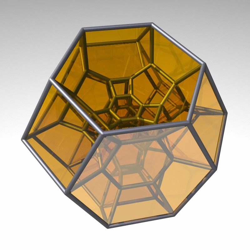
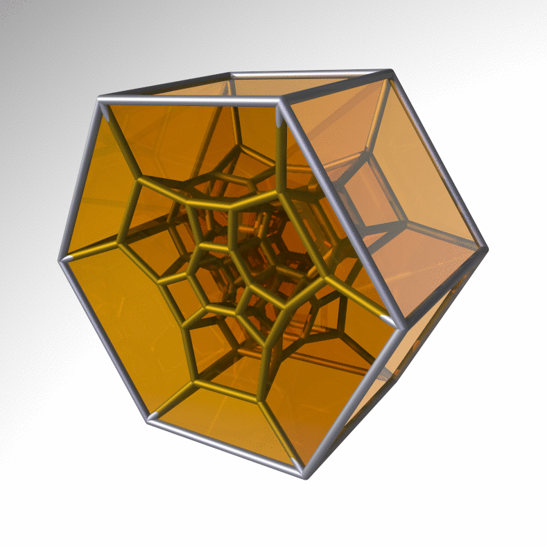
Figure 1. Schlegel diagrams of the $4$-permutohedron with respect to two different facets: a $3$-permutohedron (left) and a prism over a hexagon (right).

Remark 6.

The Schlegel diagram construction shows that the vertex-edge graphs of $3$-polytopes are planar; see Theorem 1.

Remark 7.

Consider the moment curve $m:t\mapsto(t,t^{2},t^{3},t^{4})$ in ${\mathbb{R}}^{4}$. Taking $n$ distinct values $t_{1}<t_{2}<\dots<t_{n}$, the convex hull $\operatorname{conv}\{m(t_{1}),m(t_{2}),\dots,m(t_{n})\}$ of the corresponding points is a cyclic $4$-polytope on $n$ vertices. As a special feature the vertex-edge graph of a cyclic $4$-polytope is isomorphic to the complete graph. Since each finite graph is a subgraph of a complete graph, the Schlegel diagram construction establishes that each finite graph admits a drawing in ${\mathbb{R}}^{3}$ without self-intersections. The cyclic polytopes are simplicial.

Since the geometry of the projection facet is preserved under the projection we cannot expect to get a “nice” Schlegel diagram right away. For some polytopes there may be a good choice of a facet and a point beyond, but this choice may not be obvious. The next section discusses how to find a good Schlegel diagram interactively.

3.1. Obtaining all Schlegel Diagrams of a Polytope

The Schlegel diagram of a polytope $P$ depends on the projection facet $F$ and the point $v$ beyond $F$, the viewpoint. To obtain all Schlegel diagrams of a $4$-polytope we start with any Schlegel diagram and describe an interactive method to choose a different projection facet and a different point beyond. This is implemented in polymake’s interface to JavaView [21] and JReality [12].

Since each facet is uniquely determined by its vertex set and all vertices are visible in the Schlegel diagram, we are able to select the vertex set of another facet in the Schlegel diagram ${\mathcal{D}}\left(P,F\right)$. In fact, it suffices to mark sufficiently many vertices, such that a unique facet containing them remains. In the JavaView and JReality graphical interfaces the user can mark points, and then press a button to get a new window with a Schlegel diagram with respect to the facet defined by the marked points. An error is issued if the facet is not uniquely specified.

It is more subtle to move the point beyond. The simple reason for this is that it does not appear in the $3$-dimensional Schlegel diagram nor its affine span. Thus it must be moved implicitly. In the beginning we choose a fixed point $w$ in the relative interior of the projection facet $F$. And we also choose a vector $r$ such that $w+{\mathbb{R}}_{\geq 0}r\cap\partial P=\{w\}$. That is, $r$ points from $w$ towards the set of points beyond $F$. For $r$ we can take an outward pointing normal vector of $F$; see Figure 2.

\begin{overpic}[width=184.9429pt]{schlegel_3d_B} \put(28.0,70.5){$v$} \put(19.5,70.0){$r$} \put(48.0,56.5){$w$} \end{overpic}

Figure 2. Construction of a Schlegel diagram of the regular octahedron. The viewpoint $v$ lies in the region beyond the projection facet. It is described by its relative position on the ray $w+{\mathbb{R}}_{\geq 0}r$.

Two cases are to be distinguished. First let us assume that the set of points beyond $F$ is bounded, that is, there is a maximal $\lambda>0$ such that $w+\zeta\lambda r$ is beyond $F$ for all $\zeta\in(0,1)$. We call $\zeta$ the zoom value of the viewpoint $v=w+\zeta\lambda r$ with respect to $w$ and $r$. The zoom value can be changed directly in the graphical interface to obtain the Schlegel diagrams for viewpoints on the segment $w+[0,\lambda]r$; see Figure 3. If, however, there is no such maximal $\lambda$ the interval of $\zeta$ is mapped from $(0,1)$ to $(0,+\infty)$ by $\zeta\mapsto\tfrac{\zeta}{1-\zeta}$.

\begin{overpic}[width=208.13574pt]{schlegel_zoom} \put(7.0,39.5){$v^{\prime}$} \put(27.0,37.0){$v$} \put(47.0,33.0){$w$} \end{overpic}

Figure 3. The construction of the Schlegel diagram of a pentagon (shaded) on one of its facets (vertical edge). The zoom parameter allows to move the old viewpoint $v$ to a new viewpoint $v^{\prime}$ on the ray connecting viewpoint and the point $w$ on the facet.

Other Schlegel diagrams are obtained by dragging individual points in the projection. There are surely different ways to move the viewpoint in the entire region beyond the projection facet by interpreting the dragging of the vertices of the Schlegel diagram. Our choice proved to be intuitive and very useful for our applications. It works as follows. If a vertex of the projection facet $F$ is dragged, the current viewpoint $v$ and the point $w$ are moved in opposite directions; see Figure 4 (left). If, however, a point $\pi(x)$ is moved, where $x$ is a vertex not belonging to $F$, only the viewpoint $v$ is modified. Then the dragged point becomes the projection of $x$ in the modified Schlegel diagram; see Figure 4 (right). Since we require that $v$ can only be moved parallel to $F$, this uniquely defines the new viewpoint $v^{\prime}$ as the intersection of the line through $x$ and $\pi(x)$ with the affine hyperplane through $v$ which is parallel to $F$.

\begin{overpic}[width=433.62pt]{schlegel_move_outer} \put(15.0,30.0){$v$} \put(15.0,47.0){$v^{\prime}$} \put(28.0,4.0){{\color[rgb]{1,0,0}move}} \end{overpic}

\begin{overpic}[width=433.62pt]{schlegel_move_inner} \put(20.0,26.0){$v$} \put(20.0,52.0){$v^{\prime}$} \put(46.0,16.0){{\color[rgb]{1,0,0}move}} \end{overpic}

Figure 4. A pentagon with its Schlegel diagram on one of its facets. The movement of the vertices in the Schlegel diagram is translated into movement of the viewpoint, which does not appear in the diagram. The movement depends on whether the point moved lies on the projection facet (left) or not (right).

This approach allows to produce all possible Schlegel diagrams. In the implementation it is always verified that the new viewpoints lead to valid Schlegel diagrams, that is, the new viewpoints remain to be points beyond $F$.

4. Pseudo-Physical Models

So far we were concerned with the visualization of (low-dimensional) polytopes, where we had natural ways of visualizing, either directly or via Schlegel diagrams. In higher dimensions or if only the face poset of a polytope is given (but no coordinates) other techniques are required. In the following we concentrate on visualizing the vertex-edge graph of a polytope. At least if the polytope is simple this can be expected to be fruitful in view of Theorem 3.

A frequently followed approach is via models copied from physics. This way often nice drawings can be obtained since the inherent symmetry properties of physical laws tend to retain the abstract symmetry of a graph in its drawings. Another great advantage of such pseudo-physical models is that forces may be added to improve an existing model. On the other hand, evolution in time of the pseudo-physical model has to be approximated and convergence to a stable state is not guaranteed due to the discretization of time; for a more thorough discussion see Fruchtermann and Reingold [9] or Tollis et al. [27, Chapter 10].

4.1. Attracting and Repellent Forces

We want to visualize a finite graph $G=(V,E)$. The naive idea is to assign random coordinates to each node $v\in V$ and then to let some “forces” act on the points until an equilibrium is reached. The neighbors of a node $v\in V$ form the set $N(v)=\{w\in V\,|\,\{v,w\}\in E\}$, its closed neighborhood is $N[v]=N(v)\cup\{v\}$.

At a given time each node of $G$ is represented by some point in ${\mathbb{R}}^{3}$. In the formulae below we will identify each node with its coordinates in $3$-space. Firstly we define a repellent force $\tfrac{-\delta_{\text{rep}}}{\|w-v\|^{3}}(w-v)$ pushing $v$ away from any non-neighboring node $w\in V(G)\setminus N[v]$. One may think of this repellent force as resulting from a (kind of) negative electronic charge carried by the vertices. Then $\delta_{\text{rep}}$ is the electrostatic constant in the repellent force. On the other hand, the edge $\{v,w\}$ for each adjacent node $w\in N(v)$ pulls $v$ towards $w$ like a stretched spring. Thus an attracting force of $\Big{(}\tfrac{1}{\ell_{\{v,w\}}}-\tfrac{1}{\|w-v\|}\Big{)}(w-v)$ acts on $v$, where $\ell_{\{v,w\}}$ is the desired length of the spring modeling the edge $\{v,w\}$. Depending on the situation this desired length may be constant (for instance, if no coordinates are known) or it may reflect some geometric properties (such as the Euclidean distance in some high-dimensional space). Note that the exact formulation of the attracting and repelling forces described above does not strictly reflect some physical model but also takes into account experimental fine tuning. Summing up the attracting and repelling forces for $v$ yields

(1) $$f_{v}\ =\ \sum_{w\in V\setminus N[v]}\frac{-\delta_{\text{rep}}}{\|w-v\|^{3}}(w-v)\ +\ \sum_{w\in N(v)}\Big{(}\tfrac{1}{\ell_{\{v,w\}}}-\tfrac{1}{\|w-v\|}\Big{)}(w-v)\,.$$

This defines a discrete vector field on the finite point set representing the node set $V$.

In order to facilitate convergence we add inertia and viscosity to our dynamical system. Adding inertia means to take the first derivative of the motion of each node into account. Adding viscosity means to systematically decrease the total energy of the system. This will be achieved by scaling down the inertia by a constant $\delta_{\text{visc}}$. The dynamics are modeled by a rather crude discretization of time. This can result in convergence problems, which may be avoided by using more advanced numerics. However, for the scope of this paper a simple discretization will suffice.

Let $v_{i}$ denote the coordinate vector of a node $v$ at time $i$. Then the new coordinate vector $v_{i+1}$ is given by

$$v_{i+1}\ =\ v_{i}+f_{v_{i}}+\delta_{\text{visc}}(v_{i}-v_{i-1})\,.$$

As a start configuration choose any random distribution of the nodes on the unit sphere with inertia zero. The simulation is run till the absolute fluctuation

$$\max_{v\in V(G)}\|v_{i}-v_{i+1}\|^{2}$$

drops below some fixed threshold. So far the pseudo-physical model is quite standard, and it does not reflect any special properties of polytopal graphs.

Example 8.

Bern, Eppstein et al. [3, 8] construct 3-dimensional zonotopes with central 2D-sections of quadratic size with respect to the number of zones (the data defining a zonotope). These $3$-zonotopes are remarkable since naively one might expect only a linear number of vertices in any section of a “typical” $3$-dimensional zonotope. Their duals are dual 3-zonotopes with $n$ zones and a $2$-dimensional affine image (a $2$D-shadow) with $\Omega(n^{2})$ vertices. Koltun [29, Problem 3] asked for a generalization, that is, dual $d$-zonotopes with $n$ zones and 2D-shadows of size $\Omega(n^{d-1})$ (for fixed $d$). Note that there is a trivial upper bound of $O(n^{d-1})$ for the size of a maximal 2D-shadow since dual $d$-zonotopes correspond to affine $(d-1)$-dimensional hyperplane arrangements. Such dual $d$-zonotopes with 2D-shadow of size $\Omega(n^{d-1})$ exist by [23]. A $3$-dimensional example is used in Figure 5 to illustrate the use of different desired edge lengths in the spring embedder. This is a particularly challenging case for our pseudo-physical model because of the great length differences.

   

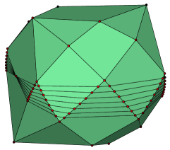
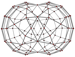
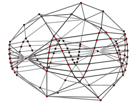
Figure 5. A dual 3-zonotope embedded with its original coordinates (left) and two spring embeddings of its graph (center and right). In the center drawing all edges are given the same desired edge lengths, on the right an attempt to embed each edge with its original length.

However, one can modify such a pseudo-physical model by inventing further forces. Here we will pursue how to visualize the vertex-edge graph $G=\Gamma(P)$ of a polytope $P\subset{\mathbb{R}}^{d}$ if additionally a linear objective function $\lambda:{\mathbb{R}}^{d}\to{\mathbb{R}}$ is given. Without loss of generality we can assume that $\lambda$ projects a point $x\in{\mathbb{R}}^{d}$ to its last coordinate $x_{d}$. The effect of the additional force $f_{F}$ may be interpreted as a (vertical) linear field: Every vertex $v\in G$ tries to adopt its $x_{3}$-coordinate $v_{3}$ (relative to the other vertices) according to its (relative) value with respect to $\lambda$. To this end the center of gravity $\bar{v}=\tfrac{1}{|V|}\sum_{v\in V}v$ of all vertices $V=V(G)$ and the average value $\bar{\lambda}=\tfrac{1}{|V|}\sum_{v\in V}\lambda(v)$ is computed. Then the additional vertical force ($e_{3}$ being the third unit vector)

$$\big{(}(\lambda(v)-\bar{\lambda})-(v-\bar{v})_{3}\big{)}e_{3}\,,$$

scaled by some constant $\delta_{\text{lin}}$, is added to the Equation (1).

All the constants mentioned, such as $\delta_{\text{rep}}$, $\delta_{\text{visc}}$, and $\delta_{\text{lin}}$, are non-negative. They must often be chosen interactively in order to balance the forces according to esthetic needs; this functionality is provided by polymake’s interfaces to JavaView and JReality.

Example 9.

The Klee-Minty cube [19, 15] is a $d$-dimensional polytope which is combinatorially isomorphic to the regular $d$-cube. It is defined as the set of admissible solutions of the linear program (maximizing $x_{d}$) given by the $2d$ inequalities

(2) $$0 \leq\!\!\! x_{1} \leq 1$$

$$\tfrac{1}{3}x_{i} \leq\!\!\! x_{i+1} \leq 1-\tfrac{1}{3}x_{i}\quad\text{for $1\leq i<d$.}$$

The Klee-Minty cube has an ascending path of length $2^{d}$, that is, there exists a directed path of length $2^{d}$ in its graph such that any vertex of this path has greater $x_{d}$-value than its predecessor. This provides an example of a polytope with an exponentially long (with respect to the number of defining halfspaces) ascending path and thus a “bad case” for the simplex algorithm; see Figure 6 (left).

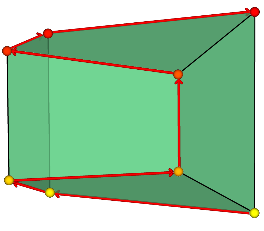
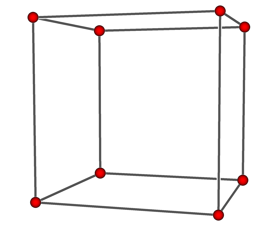
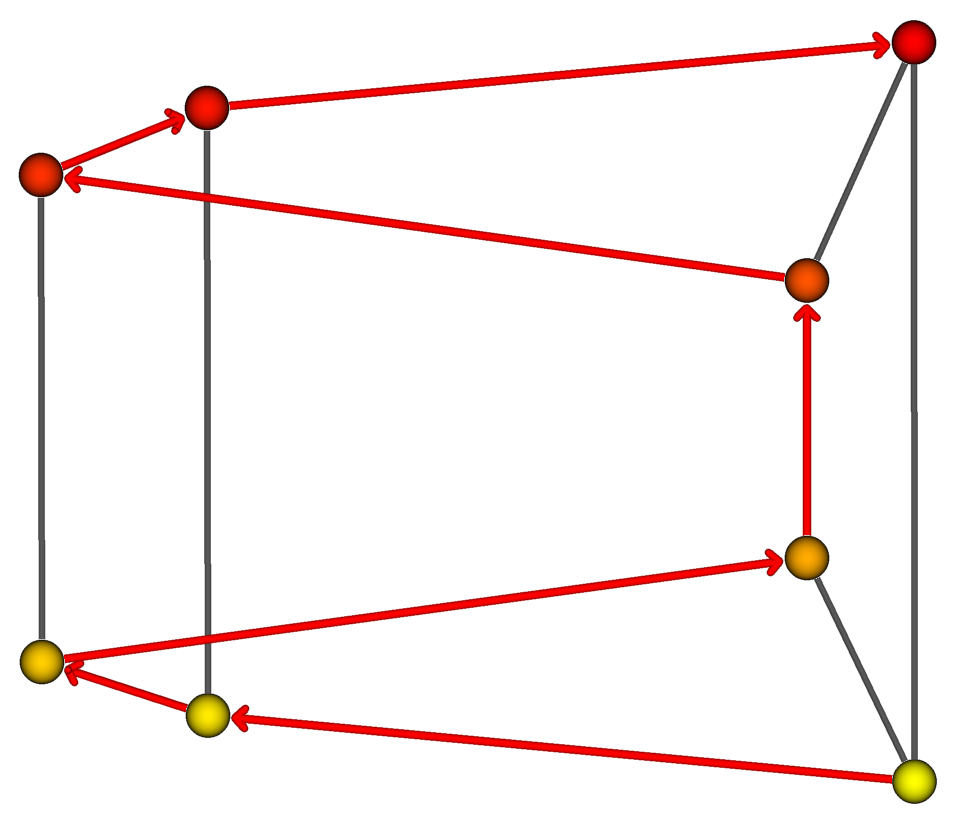
Figure 6. The Klee-Minty 3-cube (with its realization given by Equation (2)) and an ascending Hamiltonian path on the left. On the right two embedding of its graph, first without additional forces, then with an additional vertical force determined by the linear objective function ${\mathbb{R}}^{3}\to{\mathbb{R}}:x\mapsto x_{3}$.

We choose the 3-dimensional Klee-Minty cube to illustrate the effect of the vertical force governed by the linear objective function ${\mathbb{R}}^{3}\to{\mathbb{R}}:x\mapsto x_{3}$. Of course, a 3-dimensional polytope may be visualized directly; see Figure 6 (left). However, Figure 6 (center and right) exhibits the effect of the additional vertical force: The drawing in the center does not reflect the particular realization of the Klee-Minty cube, the embedding on the right on the other hand clearly shows the ascending Hamiltonian path.

Example 10.

We want to visualize the product $\Delta_{2}\times C_{3}$ of a triangle and the $3$-dimensional unit-cube. This is a $5$-dimensional simple polytope. We choose a linear objective function $\lambda:{\mathbb{R}}^{5}\to{\mathbb{R}}$ such that $\lambda$ evaluates to distinct values on the vertices of $\Delta_{2}$, but does not distinguish in between the vertices of $C_{3}$. For example let $\lambda(x)=l_{1}x_{1}+l_{2}x_{2}$ for random values $l_{1},l_{2}\in{\mathbb{R}}$. Hence for a vertex $v$ of $\Delta_{2}$ all vertices of the type “$v$ times any vertex of $C_{3}$” are embedded with the same $x_{3}$-coordinate by the vertical force. Figure 7 depicts a spring embedding of the graph of $\Delta_{2}\times C_{3}$ without additional forces on the left, and on the right with $\lambda$ taken into account. The image on the right clearly shows the three (flat horizontal) copies of $C_{3}$ corresponding to the three vertices of $\Delta_{2}$, which in turn provide the second factor of the three “edge times cube” facets of $\Delta_{2}\times C_{3}$.

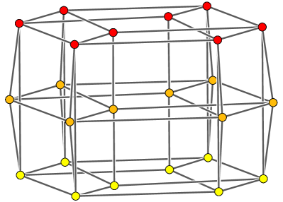
Figure 7. Two embeddings of the graph of the product of a triangle and the 3-cube. The product $\Delta_{2}\times C_{3}$ has six “triangle $\times$ square” facets (emphasized on the left) and three “edge $\times$ cube” facets (emphasized on the right).

4.2. Rubber Bands

In the following we take a different approach to embedding of graphs in ${\mathbb{R}}^{3}$. Rather than working with a dynamic model as in Section 4.1, we present a classical method due to Maxwell [20] and Cremona [6]. Here a graph $G$ is embedded into ${\mathbb{R}}^{3}$ by solving a system of linear equations. This method requires some nodes $\Phi$ already embedded in ${\mathbb{R}}^{3}$. The graph $G$ will be embedded in the affine subspace spanned by the nodes in $\Phi$. Hence it is often useful to require that $\Phi$ contains at least four nodes which span the whole space. Further we assume $G$ to be connected, since we may embed different connected components individually.

We picture an edge $e\in E(G)$ as a spring, or a rubber band, of length zero (if not stretched); the edge $e$ has an individual spring constant $\delta_{e}$. After fixing coordinates for the nodes in $\Phi$ we let the rubber bands pull the remaining nodes to an equilibrium. This equilibrium is attained by minimizing the total energy $E$ of the system of rubber bands. To this end let $v_{1}$, $v_{2}$, and $v_{3}$ be the coordinates in ${\mathbb{R}}^{3}$ of a node $v\in V(G)$ and the energy of a rubber band representing an embedded edge $e$ is $\delta_{e}\|e\|^{2}$. Hence we have

$$E\ =\ \sum_{e\in E(G)}\delta_{e}\|e\|^{2}\ =\ \frac{1}{2}\sum_{v\in V(E)}\sum_{w\in N(v)}\delta_{\{v,w\}}\left\|\begin{pmatrix}v_{1}-w_{1}\\ v_{2}-w_{2}\\ v_{3}-w_{3}\end{pmatrix}\right\|^{2}\,.$$

The total energy $E$ is a quadratic function in $3|V(G)\setminus\Phi|$ variables $v_{1}$, $v_{2}$, and $v_{3}$ for all $v\in V(G)\setminus\Phi$ and thus $E$ has a unique minimum. Partial differentiation with respect to $v_{1}$ yields

$$\frac{\partial E}{\partial v_{1}}\ =\ 2\sum_{w\in N(v)}\delta_{\{v,w\}}(v_{1}-w_{1})\,,$$

and likewise for $v_{2}$ and $v_{3}$. Requiring equilibrium, that is, $\frac{\partial E}{\partial v_{1}}=\frac{\partial E}{\partial v_{2}}=\frac{\partial E}{\partial v_{3}}=0$ for all $v\in V(G)\setminus\Phi$, amounts to solving a system of $3|V(G)\setminus\Phi|$ linear equations to determine the values of $v_{1}$, $v_{2}$, and $v_{3}$ for all $v\in V(G)\setminus\Phi$.

This technique was applied by Tutte [28] to construct crossing free embeddings of connected planar graphs into ${\mathbb{R}}^{2}$ with straight edges. Here $v_{3}$ is set to zero for all nodes $v$ to obtain an embedding in ${\mathbb{R}}^{2}$.

The same method can also be used to prove the difficult direction of Steinitz’ Theorem (Theorem 1): The construction of a 3-polytope from a given planar, 3-connected graph. In the following we sketch the idea. Let $G$ be a $3$-connected planar graph. Then $G$ or its dual graph $G^{*}$ possesses a triangular face. This can be derived from Euler’s theorem and double counting. It suffices to prove that $G$ or $G^{*}$ is the vertex-edge graph of some $3$-polytope $P$ because the polar dual of $P$ has the dual graph as its vertex-edge graph. So we can safely assume that $G$ has a triangular face. Fix its nodes in general position in ${\mathbb{R}}^{2}$. Now we embed $G$ in ${\mathbb{R}}^{2}$ using Tutte’s rubber band method. According to Maxwell [20] such an embedding may be lifted into ${\mathbb{R}}^{3}$, that is, there exists a convex function ${\mathbb{R}}^{2}\rightarrow{\mathbb{R}}$ which is linear on the faces of the planar embedding of $G$. The polytope $P$ with $G$ at its graph is the convex hull of the lifted nodes of $G$. Since we fixed the coordinates of a triangular face of $G$ to begin with our rubber band method, no new edges arise in the convex hull $P$ and $G=\Gamma(P)$ holds. See Figure 8 for a realization of the icosahedron obtained from its graph via the rubber band method. For a detailed proof see Richter-Gebert [22, Sect. 13.1].

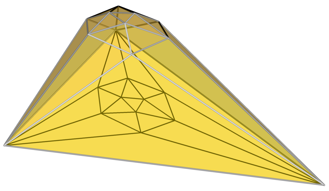
Figure 8. Non-regular realization of the icosahedron obtained from its graph via the rubber band method. The rubber band embedding of the graph is visualized as the shadow of the edges of the icosahedron.

Notice that Tutte’s rubber band embedding of $G$ is a Schlegel diagram of the lifted polytope $P$ (with a viewpoint at infinity).

5. Applications

In contrast to what we discussed so far we will now study the visualization of geometric objects which are more loosely connected to polytopes. In most cases we will deal with visualizing graphs by the pseudo-physical approach from Section 4.1 with additional forces which are specific to the application intended.

5.1. Tight Spans of Finite Metric Spaces

Let $\delta:T\times T\to{\mathbb{R}}_{\geq 0}$ be a metric on a finite set $T=\{t_{1},\dots,t_{n}\}$ of taxa. Then one can associate to it the convex polyhedron

$$P_{\delta}\ =\ \left\{x\in{\mathbb{R}}^{n}\vphantom{x_{i}+x_{j}\geq\delta(t_{i},t_{j})\text{ for all $i,j$}}\,\right.\left|\,\vphantom{x\in{\mathbb{R}}^{n}}x_{i}+x_{j}\geq\delta(t_{i},t_{j})\text{ for all $i,j$}\right\}\,.$$

Because of $\delta(t_{i},t_{i})=0$ the polyhedron $P_{\delta}$ is contained in the positive orthant ${\mathbb{R}}_{\geq 0}^{n}$, and hence it is pointed, that is, it does not contain any affine line. Moreover, $P_{\delta}$ is always non-empty and unbounded, since the ray ${\mathbb{R}}_{\geq 0}(M,\dots,M)$ is contained in $P_{\delta}$, where $M$ is the maximal value attained by the metric $\delta$. The polytopal subcomplex of all those faces which are bounded, the bounded subcomplex of $P_{\delta}$, is denoted by ${\mathcal{T}}(P_{\delta})$. Bandelt and Dress [2] introduced the name tight span for these objects, but they already showed up earlier as the injective envelope of a metric space in the work of Isbell [14]. Note that the bounded subcomplex of an unbounded polyhedron is always contractible. Tight spans of finite metric spaces are dual to regular subdivisions of second hypersimplices.

The interest in this construction comes from the following simple observation.

Proposition 11.

The polytopal complex ${\mathcal{T}}(P_{\delta})$ is $1$-dimensional, that is, it consists of edges only, if and only if the metric $d$ is tree-like.

Here a metric is called tree-like if it arises from a finite tree, that is, a connected graph without cycles, with non-negative weights associated to the edges. Between any two nodes in a tree there is a unique shortest path, and hence, by adding up all the weights on a shortest path, this gives a distance function on the set of nodes. As there are no cycles, there are no proper triangles, and the triangle inequality is trivially satisfied. The tight span of such a tree-like metric itself (essentially) is the tree. Moreover, the whole construction of the tight span depends on the metric in a continuous way. Hence, a tight span is a geometric object which can be used to measure in how far a given metric is tree-like. This very property can be exploited for an interesting application.

The goal of phylogenetics, as a subject in biology, is to determine evolutionary kinship among species or individual organisms. Methods include the inspection of fossil samples, the morphological analysis of extinct and existing species, and the study of ontogenetic development on organisms. One approach, which became feasible with the advent of modern sequencing techniques, is to extract genetic distance information from alignments of DNA or amino acid sequences. Again there is a choice of mathematical models which try to associate a tree with the given sequences. But the beauty of the tight span approach lies in the possibility to detect whether it makes sense to associate any tree with the given metric to begin with. In this sense tight span based techniques are less biased than several other methods.

As far as the visualization is concerned several choices can be made. For instance, one can use the plain pseudo-physical model from Section 4.1. However, this combinatorial visualization does not provide us with images which are meaningful in the context of phylogenetics. For this it is better to set the desired edge lengths in (1) to edge lengths related to the distance function. It turns out that the taxa arise as specific vertices of the polyhedron $P_{\delta}$, and the proper desired edge length is the distance with respect to maximum norm between two vertices of $P_{\delta}$. We call this the approximate metric visualization of a tight span.

Example 12.

Consider a metric $\delta$ on eight taxa which happens to be induced by aligned RNA-samples of eight different species, five of which being algae. The complete data set is taken from the example file algae.nex which comes with SplitsTree [13]. Note that the RNA samples used are very short: They come from 920 bases each. There is more than one way to compute a distance function from these samples; here we used SplitsTree’s method UncorrectedP to arrive at a metric given by the upper triangular matrix

$$\small\left(\begin{array}[]{llllllll}0.0&0.026&0.029&0.112&0.078&0.136&0.123&0.141\\ &0.0&0.041&0.121&0.088&0.144&0.132&0.145\\ &&0.0&0.099&0.064&0.123&0.121&0.133\\ &&&0.0&0.1&0.142&0.143&0.156\\ &&&&0.0&0.116&0.118&0.116\\ &&&&&0.0&0.159&0.135\\ &&&&&&0.0&0.136\\ &&&&&&&0.0\\ \end{array}\right)\,,$$

where the rows and columns are labeled with the following ordered list of taxa: tobacco, rice, marchantia, chlamydomonas, chlorella, euglena, anacystis nidulans, olithodiscus.

The left picture in Figure 9 shows a combinatorial visualization of the graph of ${\mathcal{T}}(P_{\delta})$. The eight taxa can be associated with vertices of $P_{\delta}$ and hence occur as nodes of the graph. The colors of the edges visualize the highest dimension of a bounded face containing that edge. By default “red” refers to dimension $1$ and “blue” to the maximum dimension $\dim{\mathcal{T}}(P_{\delta})$, which equals $4$ in this case. The two shades of purple refer to dimensions $2$ and $3$, respectively.

The picture to the right is the approximate metric visualization of ${\mathcal{T}}(P_{\delta})$. No color coding for the edges in this case. The sample is too small to deduce much about the evolutionary relationship between the five kinds of algae, but it already suffices to tell the algae apart from the non-algae species.

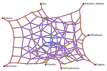
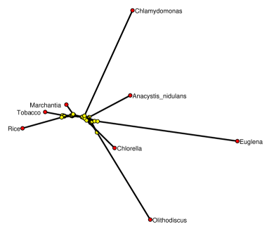
Figure 9. Left: Combinatorial visualizing of the tight span of five species of algae (chlamydomonas, chlorella, euglena, anacystis nidulans, olithodiscus) and three non-algae (tobacco, rice, marchantia). Right: Approximate metric visualization of the same tight span.

The visualization of tight spans used by Sturmfels and Yu is the combinatorial one [26].

5.2. Tropical Polytopes

Consider a matrix $C=(c_{ij})\in{\mathbb{R}}^{m\times n}$, and let $W={\mathbb{R}}^{m+n}/{\mathbb{R}}(1,1,\dots,1,-1,-1,\dots,-1)$ be a (quotient) vector space of dimension $m+n-1$. Each point in $W$ is written as a pair $(y,z)$ where $y$ takes the first $m$ coordinates, and $z$ the remaining $n$. Note that, in the quotient $W$, the equation $(y+(1,1,\dots,1),z-(1,1,\dots,1))=(y,z)$ holds. Now

(3) $$T_{C}\ =\ \left\{(y,z)\in W\vphantom{y_{i}+z_{j}\leq c_{ij}}\,\right.\left|\,\vphantom{(y,z)\in W}y_{i}+z_{j}\leq c_{ij}\right\}$$

is a pointed unbounded convex polyhedron. The bounded subcomplex ${\mathcal{T}}(T_{C})\subset W$ is the tropical polytope generated by (the rows of) $C$. The vertices of $T_{C}$ are called the tropical pseudo-vertices of ${\mathcal{T}}(T_{C})$ with respect to the rows of $C$. Among these there is a unique inclusion-minimal subset which generates the tropical polytope: the tropical vertices of ${\mathcal{T}}(T_{C})$. Tropical polytopes are dual to regular subdivisions of products of simplices. For details on the subject see [7, 16, 5].

As it turns out, projecting $T_{C}$ onto the first $m$ coordinates (or onto the last $n$ coordinates) and clearing the first remaining coordinate (by adding a suitable multiple of $(1,1,\dots,1)$) yields an affine isomorphism. This way, one has a direct visualization in ${\mathbb{R}}^{3}$ if $\min(m,n)\leq 4$.

Example 13.

Letting

(4) $$C\ =\ \begin{pmatrix}1&0&0\\ 0&1&0\\ 0&\tfrac{1}{4}&1\end{pmatrix}$$

gives the tropical triangle ${\mathcal{T}}(T_{C})$, where $m=n=3$, in Figure 10 (left). Its vertices correspond to the rows of the matrix $C$.

Example 14.

If we form the $(n!\times n)$-matrix whose rows are the permutation vectors from Example 5 the construction (3) gives the tropical $(n-1)$-permutohedron. Figure 10 (right) shows the tropical $3$-permutohedron; the unit grid in the background is meant to provide a better idea about the spatial proportions.

\begin{overpic}[width=195.12767pt]{trop-3gon} \put(4.0,-1.0){\small$(1,0,0)=(0,-1,-1)$} \put(87.7,42.1){\small$(0,1,0)$} \put(63.0,95.0){\small$(0,\tfrac{1}{4},1)$} \end{overpic}

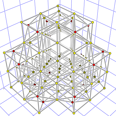
Figure 10. Left: Tropical triangle ${\mathcal{T}}(T_{C})$, where $C$ is defined in (4). Right: Tropical $3$-permutohedron.

Since tropical polytopes are so similar to tight spans of finite metric spaces the same visualization techniques can be applied in higher dimensions. However, for the tropical polytopes the combinatorial information is usually of interest. This is why the combinatorial visualization (with constant desired edge length) is preferred.

Example 15.

For $M(m,n)=(\mu_{ij})\in{\mathbb{Z}}^{m\times(n+1)}$ with $\mu_{ij}=ij$ the bounded subcomplex ${\mathcal{T}}(T_{M(m,n)})$ is the tropical cyclic polytope with $m$ vertices in dimension $n$ [5]. The case $m=6$ and $n=4$ is shown in Figure 11. The tropical cyclic polytope ${\mathcal{T}}(T_{M(4,6)})$ has $126$ pseudo-vertices, six of which are tropical vertices.

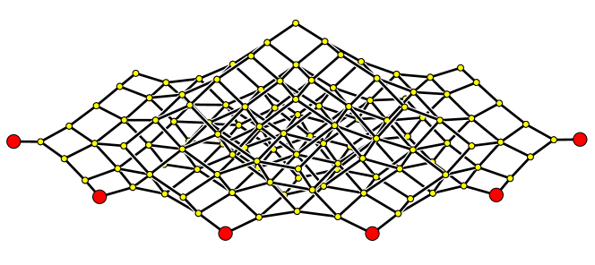
Figure 11. Tropical cyclic $4$-polytope with six tropical vertices (red).

5.3. pd-Graphs of Simplicial Manifolds

Natural candidates for graphs to associate with a finite simplicial complex are its $1$-skeleton (also called the primal graph) and its dual graph. They both encode neighborhood information, the adjacency of vertices in the primal graph, and the adjacency of facets in the dual graph. But each carries only incomplete information: The primal graph does not “see” the facets, that is, we do not know which set of vertices of the graph forms a face (of dimension higher than one) and which does not. On the other hand, we cannot tell from the dual graph if facets intersect, unless the intersection is a ridge. Thus it is sometimes useful to combine the two graphs in a common picture. This allows us to find a more “accurate” embedding of the graphs since we may be able to make use of the two kind of adjacency informations at the same time. This approach will sometimes allow for pictures of not too high-dimensional objects which carry some geometric meaning.

We define the primal-dual graph, or pd-graph for short, as the disjoint union of the primal and the dual graph with the following additional edges: A primal node corresponding to a vertex $v$ and a dual node corresponding to facet $F$ are connected by an artificial edge if $v\in F$.

Example 16.

Consider an abstract simplicial complex $K$ homeomorphic to a solid whose boundary surface is of genus $2$. A priori there are no coordinates for the vertices of $K$ given, but using our pseudo-physical model (following Section 4.1) on the pd-graph of $K$ we nevertheless are able to produce a decent picture, clearly showing the two holes of $K$; see Figure 12. Here the artificial edges are removed to show only the primal and the dual graph. If we choose the desired edge lengths of the artificial edges sufficiently small, then each dual node (corresponding to a facet $F$) is pulled into the interior of the simplex defined by the nodes corresponding to the vertices of $F$.

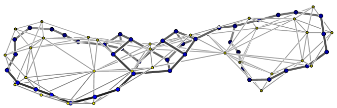
Figure 12. pd-graph of a triangulation of a solid surface of genus 2. The thin edges belong to the primal graph, and the thick ones to the dual.

Example 17.

Figure 13 depicts the unique facet-minimal triangulation of the 4-cube $C_{4}=[0,1]^{4}$. The triangulation has no additional vertices and 16 facets. The entire $f$-vector reads $(16,57,86,60,16)$. One way to visualize this triangulation of $C_{4}$ is to look at the triangulation induced on the boundary of $C_{4}$ in its Schlegel Diagram; see Section 3. Schlegel diagrams preserve combinatorial data as well as geometric information. But they project the polytope to one of its facets, hence only the boundary is visualized and all the information about the triangulation in the interior is lost.

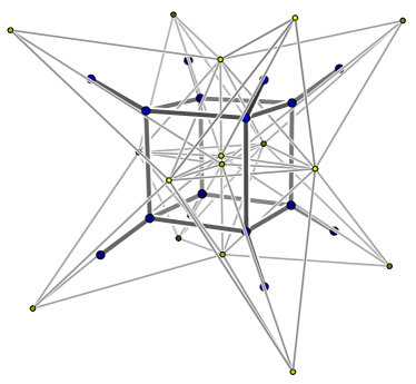
Figure 13. pd-graph of the unique facet-minimal triangulation of $C_{4}$.

Alternatively, we embed the pd-graph of the minimal triangulation of $C_{4}$ via the spring embedder. Any image of a higher than 3-dimensional object has to be admired with care. Nevertheless one can identify the facets of the minimal triangulation of $C_{4}$ and the way they intersect in the embedding of the pd-graph in Figure 13.

6. Acknowledgments

We are grateful to Ronald Wotzlaw for his beautiful regular realization of the $4$-dimensional permutohedron which led to Figure 1.

References

- [1] M. L. Balinski, On the graph structure of convex polyhedra in -space, Pacific J. Math. 11 (1961), 431–434. MR MR0126765 (23 #A4059)
- [2] Hans-Jürgen Bandelt and Andreas Dress, Reconstructing the shape of a tree from observed dissimilarity data, Adv. in Appl. Math. 7 (1986), no. 3, 309–343. MR MR858908 (87k:05060)
-
[3]
Marshall Wayne Bern, David Eppstein, Leonidas J. Guibas, John E. Hershberger,
Subhash Suri, and Jan Dithmar Wolter, The centroid of points with
approximate weights, Proc. 3rd Eur. Symp. Algorithms (ESA 1995) (Paul G.
Spirakis, ed.), Lecture Notes in Computer Science, no. 979, Springer-Verlag,
September 1995,
http://www.ics.uci.edu/~eppstein/pubs/BerEppGui-ESA-95.ps.gz, pp. 460–472. - [4] Roswitha Blind and Peter Mani-Levitska, Puzzles and polytope isomorphisms, Aequationes Math. 34 (1987), no. 2-3, 287–297. MR MR921106 (89b:52008)
- [5] Florian Block and Josephine Yu, Tropical convexity via cellular resolutions, J. Algebraic Combin. 24 (2006), no. 1, 103–114. MR MR2245783 (2007f:52041)
- [6] Luigi Cremona, Graphical statics, Oxford University Press, 1890, English translation by T. H. Beare.
- [7] Mike Develin and Bernd Sturmfels, Tropical convexity, Doc. Math. 9 (2004), 1–27 (electronic), correction: ibid., pp. 205–206. MR MR2054977 (2005i:52010)
-
[8]
David Eppstein, Ukrainian easter egg, in: “The Geometry Junkyard”,
computational and recreational geometry, 23 January 1997,
http://www.ics.uci.edu/~eppstein/junkyard/ukraine/. - [9] Thomas Fruchtermann and Edward Reingold, Graph drawing by force-directed placement, Software Practice and Experience 21 (1992), no. 11, 1129–1164.
- [10] Ewgenij Gawrilow and Michael Joswig, polymake, version 2.3 (desert), 1997–2007, with contributions by T. Rörig and N. Witte, free software, http://www.math.tu-berlin.de/polymake.
- [11] Ewgenij Gawrilow and Michael Joswig, polymake: a framework for analyzing convex polytopes, Polytopes–combinatorics and computation (Oberwolfach, 1997), DMV Sem., vol. 29, Birkhäuser, Basel, 2000, pp. 43–73. MR 2001f:52033
- [12] Charles Gunn, Tim Hoffmann, Markus Schmies, and Steffen Weißmann, jReality, http://www.jreality.de, 2007.
- [13] Daniel H. Huson and David Bryant, Application of phylogenetic networks in evolutionary studies, Mol. Biol. Evol. 23 (2006), no. 2, 254–267, www.splitstree.org.
- [14] J. R. Isbell, Six theorems about injective metric spaces, Comment. Math. Helv. 39 (1964), 65–76. MR MR0182949 (32 #431)
- [15] Michael Joswig, Goldfarb’s cube, 2000, http://www.eg-models.de, eg-model nr. 2000.09.030.
- [16] Michael Joswig, Tropical halfspaces, Combinatorial and computational geometry, Math. Sci. Res. Inst. Publ., vol. 52, Cambridge Univ. Press, Cambridge, 2005, pp. 409–431. MR MR2178330 (2006g:52012)
- [17] Michael Jünger and Petra Mutzel (eds.), Graph drawing software, Mathematics and Visualization, Springer-Verlag, Berlin, 2004. MR MR2159308
- [18] Volker Kaibel and Alexander Schwartz, On the complexity of polytope isomorphism problems, Graphs Combin. 19 (2003), no. 2, 215–230. MR MR1996205 (2004e:05125)
- [19] Victor Klee and George J. Minty, How good is the simplex algorithm?, Inequalities, III (Proc. Third Sympos., Univ. California, Los Angeles, Calif., 1969; dedicated to the memory of Theodore S. Motzkin), Academic Press, New York, 1972, pp. 159–175. MR MR0332165 (48 #10492)
- [20] J. C. Maxwell, On reciprocal figures and diagrams of forces, Philosophical Magazine (1864), 250–261, Ser. 4, 27.
- [21] Konrad Polthier, Klaus Hildebrandt, Eike Preuss, and Ulrich Reitebuch, JavaView, version 3.95, http://www.javaview.de, 2007.
- [22] J. Richter-Gebert, Realization spaces of polytopes, vol. 1643, Springer Verlag, Berlin Heidelberg, 1996.
- [23] Thilo Rörig, Nikolaus Witte, and Günter M. Ziegler, Zonotopes with large 2d cuts, 2007, arXiv:0710.3116v2.
- [24] Ernst Steinitz, Polyeder und Raumteilungen, Encyklopädie der mathematischen Wissenschaften, 1922, Dritter Band: Geometrie, III.1.2., Heft 9, Kapitel 3 A B 12, pp. 1–139.
- [25] Ernst Steinitz and Hans Rademacher, Vorlesungen über die Theorie der Polyeder unter Einschluss der Elemente der Topologie, Springer-Verlag, Berlin, 1976, Reprint der 1934 Auflage, Grundlehren der Mathematischen Wissenschaften, No. 41. MR MR0430958 (55 #3962)
- [26] Bernd Sturmfels and Josephine Yu, Classification of six-point metrics, Electron. J. Combin. 11 (2004), no. 1, Research Paper 44, 16 pp. (electronic). MR MR2097310 (2005m:51016)
- [27] Ioannis G. Tollis, Giuseppe Di Battista, Peter Eades, and Roberto Tamassia, Graph drawing, Prentice Hall Inc., Upper Saddle River, NJ, 1999, Algorithms for the visualization of graphs. MR MR2064104 (2005i:68067)
- [28] W. T. Tutte, How to draw a graph, Proc. London Math. Soc. 13 (1963), no. 3, 743–767.
- [29] Uli Wagner (ed.), Conference on Geometric and Topological Combinatorics: Problem Session, Oberwolfach Reports 4 (2006), no. 1, 265–267.
- [30] Günter M. Ziegler, Lectures on polytopes, Springer, 1995.