eurm10 \checkfontmsam10 \pagerange1–2
Transition in pipe flow: the saddle structure on the boundary of turbulence
Abstract
The laminar-turbulent boundary is the set separating initial conditions which relaminarise uneventfully from those which become turbulent. Phase space trajectories on this hypersurface in cylindrical pipe flow look to be chaotic and show recurring evidence of coherent structures. A general numerical technique is developed for recognising approaches to these structures and then for identifying the exact coherent solutions themselves. Numerical evidence is presented which suggests that trajectories on are organised around only a few travelling waves and their heteroclinic connections. If the flow is suitably constrained to a subspace with a discrete rotational symmetry, it is possible to find locally-attracting travelling waves embedded within . Four new types of travelling waves were found using this approach.
1 Introduction
Transition to turbulence in cylindrical pipe flow is governed by one single dimensionless parameter, the Reynolds number where is the mean flow speed along the pipe, the pipe diameter and the kinematic viscosity of the fluid (Reynolds 1883). Despite the simplicity of the set-up, the reason for transition remains obscure due to the linear stability of the laminar Hagen-Poiseuille flow (Hagen 1839, Poiseuille 1840) and the sensitivity of the process to the exact shape and amplitude of disturbances present. In most experiments, transition is observed at (e.g. Wygnanski & Champagne 1973) but can be triggered as low as (Peixinho & Mullin 2006) or delayed to in very carefully controlled experiments (Pfenniger 1961). Until recently, the only firm theoretical result was the energy stability bound of (Joseph & Carmi, 1969) below which all disturbances are guaranteed to decay monotonically. This is, however, more than an order of magnitude below the observed value for transition.
An important step forward in understanding the transition process was the discovery of disconnected solutions to the Navier-Stokes equations in a cylindrical pipe (Faisst & Eckhardt 2003, Wedin & Kerswell 2004, Kerswell 2005, Pringle & Kerswell 2007). These exact solutions are travelling waves (TWs) which appear through saddle-node bifurcations as in other shear flows (Nagata 1990, Waleffe 1997,1998,2001,2003). All these solutions are linearly unstable though they have a very low-dimensional unstable manifold. There is much interest in these solutions, as very similar structures have been observed transiently in experiments (Hof et al. 2004, 2005) and direct numerical simulations (Kerswell & Tutty 2007, Schneider et al. 2007a, Willis & Kerswell 2008a). These states can generally be divided into ‘upper-branch’ and ‘lower-branch’ TWs, based on whether they have high or low wall shear stress. Lower branch solutions are believed to sit on a hypersurface that divides phase space into two regions: one where initial points lead directly to the laminar state, the other where initial conditions lead to turbulent episodes (Kawahara 2005, Wang et. al. 2007, Kerswell & Tutty 2007, Viswanath 2008). The simple translational behaviour of these travelling wave solutions is inherent to the method used to find them, and undoubtedly masks an even larger variety of more complex exact solutions.
The boundary between laminar and turbulent trajectories - labelled
hereafter - is formally a separatrix if the turbulent state
is an attractor. At low , however, turbulence may ultimately
decay after a long transient in which case the laminar state is the
unique global attractor. Then the boundary is generalised
to the dividing set in phase space between trajectories which
smoothly relaminarise and those which do undergo a turbulent
evolution. is thought to be of codimension 1 in phase space
but one can a priori not exclude a more complex fractal
structure, as suggested by the dependence of lifetime on initial
conditions in simulations of pipe flow (Faisst & Eckhardt 2004).
Trajectories which start in - hereafter called the ‘edge’
following Skufca et al. (2006) - stay in for later times by
definition and hence the long time dynamics are of obvious interest.
The long time behaviour on has already been found to be a
periodic solution in plane Poiseuille flow in a pioneering study by
Toh & Itano (1999, see also Itano & Toh 2001). Skufca et al.
(2006) studied a 9-dimensional model of plane Couette flow (PCF) to
reveal an attracting periodic orbit at low and an apparently
chaotic state at higher . However, recent fully-resolved
simulations have shown that the asymptotic behaviour is an
attracting TW in PCF (Schneider et al. 2008, Viswanath 2008) and a
chaotic attractor in a short cylindrical pipe of length
(Schneider et al. 2007b). Interestingly, this seemingly chaotic end
state looks to be centered around an ‘asymmetric’ TW
(Pringle & Kerswell 2007, Mellibovsky & Meseguer 2007).
The purpose of this paper is to explore the dividing hypersurface in pipe flow with the following objectives:
-
1.
to establish that the dynamics restricted to this laminar-turbulent boundary explores many different saddle points embedded in it;
-
2.
to find evidence for heteroclinic or ‘relative’ homoclinic connections between these saddle points;
-
3.
to explore restricted by a discrete rotational symmetry in order to ascertain whether the limiting behaviour remains chaotic or can be a simple attractor;
-
4.
to develop a practical and general way to find TWs and periodic orbits without detailed knowledge of their spatial structure.
The works cited above employ a reduced computational domain for their calculations, imposing short-wavelength periodicity in one direction (along the pipe, Schneider et al. 2007b) or two (in the spanwise and streamwise directions in plane Couette flow, Schneider et al. 2008, Viswanath 2008). This is very much in the spirit of the Minimal Flow Unit pioneered by Jimenez & Moin (1991) and used with considerable success to identify key mechanisms underpinning turbulence (Hamilton et al. 1995). In this paper, we also adopt this same approach by concentrating on pipes up to long. The ensuing reduction in the degrees of freedom of the flow allows a much more detailed exploration of the flow dynamics albeit restricted to a subspace of strict spatial periodicity. This is a necessary preliminary to motivate a more carefully focussed study in much longer pipes which can capture spatially-localised turbulent structures (e.g. Priymak & Miyazaki 2004, Willis & Kerswell 2007, 2008a) but at considerable numerical cost still. Flow structures found in the short pipes considered here also exist, of course, in a longer pipe but will be more unstable due to the greater degrees of freedom present there. It is also worth remarking that a recent study (Nikitin 2007) has shown how pipe flow is slow to lose its spatial periodicity when this is restriction is lifted.
This paper is organised as follows. Section 2 discusses the formulation and numerical methods used to simulate the flow in a pipe and to extract exact recurrent flow solutions. Section 3 presents the results obtained using these in 7 subsections. Subsection 3.1 recalls the method used to follow trajectories on and confirms that the limiting behaviour looks chaotic (Schneider et al. 2007b). Sections 3.2 and 3.3 discuss how near-recurrent states are identified and using a Newton-Krylov algorithm demonstrate that a number of unstable travelling waves are approached. Subsection 3.4 offers evidence for the existence of a ‘relative’ homoclinic connection between a travelling wave and the same wave rotated. Subsection 3.5 looks for recurrent flow structures in restricted by a discrete rotational symmetry and identifies new exact travelling wave solutions. Subsection 3.6 shows that within this subspace the limiting state of is a simple attractor. Subsection 3.7 confirms that all the TWs found in the earlier subsections are indeed embedded in the laminar-turbulent boundary. The paper ends with a discussion in section 4.
2 Numerical Procedure
2.1 Governing Equations
We consider the incompressible flow of Newtonian fluid in a cylindrical pipe and adopt the usual set of cylindrical coordinates and velocity components . The domain considered here is , where is the length of the pipe and lengths are in units of radii (). The flow is described by the incompressible three-dimensional Navier-Stokes equations
| (1) | |||||
| (2) |
The flow is driven by a constant mass-flux condition, as in recent experiments (e.g. Peixinho & Mullin 2006). The boundary conditions are periodicity across the pipe length and no-slip on the walls .
2.2 Time-stepping code
The basic tool for the numerical determination of exact recurrent states is the accurate time-stepping code used by Willis & Kerswell (2007,2008a). The velocity field is derived from two scalar potentials and :
| (3) |
and the incompressible Navier-Stokes equations are re-written using the formulation introduced by Marqués (1990). The two scalar potentials are discretised using high-order finite differences in the radial direction and spectral Fourier expansions in the azimuthal direction and axial direction . For example, the decomposition of the scalar potential at a radial location , , reads
| (4) |
The positive integer refers to the discrete rotational symmetry
| (5) |
of the flow (trivially means no rotational symmetry is imposed). The resolution of a given calculation is described by a vector . It is adjusted until the energy in the spectral coefficients drops by at least 5 and usually 6 decades from lowest to highest-order modes. The time stepping is 2nd order accurate with updated using an adaptive method based on a CFL condition.
The number of (real) degrees of freedom, which defines the dimension of phase-space, is . The set of all complex coefficients defines our phase-space with its usual Euclidean norm . Symmetries exhibited by TWs such as the shift-and-reflect symmetry
| (6) |
and the mirror symmetry (e.g. Pringle & Kerswell 2007, Pringle et al. 2008)
| (7) |
are not imposed in the simulations.
2.3 The Newton-Krylov method
The spectral expansion defined above converts the Navier-Stokes equations into an autonomous dynamical system of the form
| (8) |
Travelling wave solutions are ‘relative equilibrium’ solutions of the Navier-Stokes, steady in an appropriate Galilean frame. It is numerically convenient to seek and interpret them as a special case of “relative periodic orbit” (RPO) (Viswanath 2007, 2008). We hence developed an algorithm to look for RPOs defined as zeros of the functional
| (9) |
Here, is the point at time on the trajectory starting at time from the point . is the point in phase space corresponding to the state shifted back in space by the distance in the axial direction and by the angle in the azimuthal direction. A shift by corresponds in phase-space to the transformation
| (10) |
A zero of corresponds to a flow repeating itself exactly after a time T, but at a different location defined by and . A travelling wave solution is a RPO where there is a degeneracy between the shifts and , and the period . For the case of a TW propagating axially with speed , , where is an apparent period. To remove this degeneracy, we impose unless otherwise specified. As the majority of known TWs do not rotate, is also assumed (those that do rotate do so rather slowly, Pringle & Kerswell, 2007). Starting from a good initial guess for and an estimate of the period (to be discussed in Section 3.2), we minimise the residual using a Newton-Krylov algorithm, based on a GMRES algorithm (Saad & Schultz, 1986). The size of the dynamical system (typically degrees of freedom) necessitates the use of a matrix-free formulation. The use of an inexact Krylov solver also leads to a significant gain in computation time (we used the choice 2 in Eisenstat & Walker, 1995). Moreover, we embed the Newton solver into a more globally convergent strategy in order to improve likeliness of convergence, using a double dogleg step technique (Dennis & Schnabel, 1995, Brown & Saad 1990). For the special case of TWs with a short period, we assume full convergence when the normalised residual is less than .
2.4 Stability of Travelling Waves
Once a travelling wave solution is known, along with its axial propagation speed , it can be expressed as a steady solution in the frame moving at speed . In this Galilean frame, the stability of the solutions can be studied numerically using an eigenvalue solver based on an Arnoldi algorithm. This yields the leading eigenvalues whose real part, when positive, indicates the growth rate of infinitesimal perturbations to the exact solution in the moving frame.
3 Results
We present 4 ‘edge’ calculations, each motivated by a different question. In the first (see §3.1-3), the edge in a pipe length () is calculated starting from a typical turbulent initial condition in order to investigate whether there are coherent structures buried in it. We are able to confirm the presence of what looks to be a chaotic attractor as found recently by Schneider et. al. (2007b). In the second edge calculation (§3.4) we look for numerical evidence of heteroclinic connections between saddle points by using a perturbed TW as an initial condition. In the third (§3.5) we impose the discrete rotational symmetry on the flow to exploit the saddle structure of the subset of to reveal new TWs which possess -symmetry. In the fourth (§3.6) we look for evidence of multiple attracting TWs to demonstrate that under a rotational symmetry constraint the large-time dynamics need not be chaotic.
3.1 Calculating Edge Trajectories
In this subsection we choose a pipe with () and , set so that there is no restriction on the rotational symmetry, and take a numerical resolution of . For this value of , turbulence, when triggered, is sustained over the typical simulation time which is much longer that the time taken to relaminarise. In order to constrain a numerical trajectory to stay on the edge surface, , we use a shooting method analogous to that first used in plane Couette flow by Toh & Itano (1999). We first produce a long turbulent trajectory and pick a state of relatively low three-dimensional disturbance energy (defined as the kinetic energy in the streamwise-dependent Fourier modes ). Initial states are then chosen from the line,
| (11) |
parameterised by the real number and is an axial average. The initial condition is two-dimensional and hence does not trigger turbulence, whereas is the original turbulent state. This -interval is then repeatedly halved with, at each stage, the new interval selected such that an initial condition corresponding to at the lower limit relaminarises, whereas that at the upper limit leads to large turbulent values of . is refined close to machine accuracy using double precision arithmetic, forcing the energy of the trajectory to stay at an intermediate level corresponding to the laminar-turbulent boundary for typical times of . At the values of used here, the energy of this boundary is clearly distinct from those associated with turbulence and thus makes determination of unambiguous. Once machine precision has been reached, the process is restarted from nearby states towards the end of the trajectory originating from neighbouring values.
The full trajectory, of duration , does not show any sign of convergence towards a simple state but rather displays erratic and unpredictable dynamics, as found by Schneider et al (2007b). We deliberately avoid the word ‘turbulent’ as this refers to larger values of . Figure 1 shows the time evolution of the .
3.2 Near-Recurrences on an Edge Trajectory
Despite the lack of regularity of the energy signals, inspection of all velocity components at several random locations in the pipe indicate clearly that the flow on is sometimes nearly periodic in time on short intervals. For the case , it is possible by eye to identify several temporal windows where all velocity components approximately oscillate with a given frequency (see Figure 2). Within these windows the dynamics on the edge appear to be temporally correlated with a short period. A large number of snapshots were taken at times across the whole trajectory. To investigate the possibility of recurrence in the flow, each snapshot state was used as an initial condition for time-stepping. The normalised distance in phase space between this initial point and its evolution in time was then examined for local minima. Specifically, we define the scalar residual function
| (12) |
where is a distance by which the state is shifted back in for comparison. We chose so that a value of for some means that the flow in the pipe is exactly the flow at time . In this case, lies on a periodic orbit of the system with the time interval being a multiple of the period (for , a vanishing residual would indicate a relative periodic orbit). For the ease of calculation, most of the time we chose to neglect the possibility of recurrence occurring after a shift in the azimuthal direction , and therefore was imposed. Typical plots of starting from different values of are displayed in Figure 3. Every function attains a smallest local minimum which is defined as
| (13) |
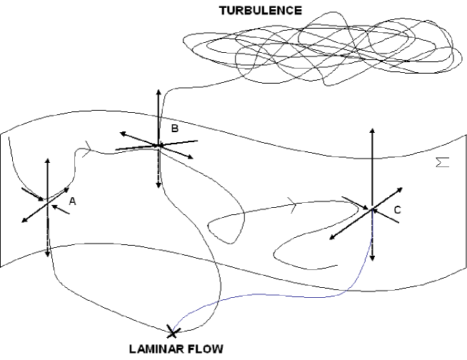
Figure 4 shows how varies with the starting point. Phases for which is small (from experience below ) may be interpreted as approximate approaches to periodic orbits of the system by the edge trajectory. The alternating pattern of maxima and minima in is then the signature of a repellor - a set of states which attract trajectories before ultimately repelling them away. For hyperbolic dynamical systems, trajectories are attracted towards one of these states along their stable manifold and ejected away along their unstable manifold (see the sketch in Figure 5). For the parameters here, 6 dips in the -profile are suggestive of 6 approaches, denoted respectively by . Parts of the trajectory linking one state to the next (e.g. or ) may be located in the vicinity of heteroclinic connections between the two states, should such a connection exist, or a relative homoclinic connection for two successive states which are the same but for a shift. The notion of ‘vicinity’ depends on the choice of the norm in phase space. Here, a pragmatic approach is adopted: we use the expression ‘ is close to a periodic orbit ’ to mean that the Newton-Krylov algorithm converges to the periodic orbit starting with the initial guess .
3.3 Exact Coherent Structures in
We now analyse the neighbourhood of the points yielding a low value of looking for exact recurrent states for which exactly vanishes. Starting from such initial guesses, the Newton-Krylov algorithm defined in §2.3 was used to further minimise . Of the six different starting guesses A to F introduced in the previous subsection, excellent convergence was obtained in the cases , , and , with being reduced down to . The converged states are labelled respectively , , and in order to distinguish them from the starting points , and to indicate the parameter . The cases and displayed only partial convergence to respectively and and it is not possible to say if there really are zeros of in this neighbourhood. Despite ‘globalisation’ improvements to the Newton-Krylov algorithm to improve convergence, sample starting guesses away from the candidates failed to converge. The converged states , , and all correspond to travelling wave solutions. Close inspection of their spatial structure and dynamics shows that they are, in fact, the same travelling wave solution modulo a shift in the azimuthal direction: see Figure 6. This state corresponds exactly to the ‘asymmetric’ TW identified in Pringle & Kerswell (2007) whose -averaged velocity field is strongly reminiscent of the chaotic state calculated by Schneider et al. (2007b). This resemblance has also been noted by Mellibovsky & Meseguer (2007) who used a different approach to infer the significance of this same asymmetric TW. Interestingly, the present study at these parameter values did not find evidence of states with higher rotational symmetry in spite of the fact that such TWs are known to be embedded in the edge (see fig. 4 of Kerswell & Tutty, 2007).
The search for recurrent states described above was initially undertaken with disallowing azimuthal propagation of the recurrent patterns. In the case , we experimented with allowing to be updated by the Newton-Raphson scheme. This involved solving an additional equation (Viswanath 2007). Using Newton-Krylov with the same starting guess but allowing the shift to be updated, produced convergence to another state which is distinct from . This state, despite a velocity profile very analogous to that of , rotates by an angle degrees after travelling one pipe length. This situation is reminiscent of the bifurcation diagram obtained by Pringle & Kerswell (2007) for the asymmetric TW (though here is much higher): for a given Reynolds number, a branch of solutions with helicity is connected to the mirror-symmetric branch, and intersects the non-helical subspace twice. The solutions at the crossing points are non-helical but nevertheless possess a rotational propagation speed , like our solution . The fact that such a solution has been found here could be explained by the fact that the numerical code used does not allow helicity, hence the Newton-Krylov algorithm has no choice but to look for the intersection of the helical branch with a non-helical subspace. However, other attempts to find exact recurrent patterns with rotation invariably converged back to a non-rotating () TW.
3.4 Search for Heteroclinic Connections
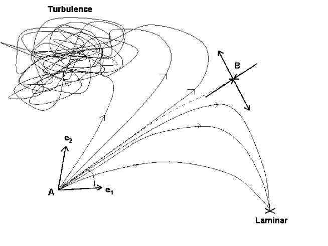
The results so far indicate the possible existence of heteroclinic trajectories linking the exact states found. When the two consecutively visited states are the same modulo a shift in the azimuthal direction, “relative” homoclinic connection is a more appropriate term. In an attempt to find further evidence for such connections, a series of initial conditions sampling the unstable manifold of a TW were explored. The asymmetric travelling wave of Pringle & Kerswell (2007) was chosen (i.e. ) with the parameters and orientated so that it was -symmetric about the plane. In the corresponding -symmetric subspace, the solution has exactly two unstable eigendirections, denoted by and , being the most unstable one (there are no unstable directions in the dual space of -antisymmetric perturbations). These two vectors were normalised to have unit energy and an initial condition was defined as
| (14) |
Here, is a positive parameter chosen small enough that is effectively in the unstable manifold of ( suffices). The angle defines a plane spanned by and and vanishes in the direction of . For some values of the angle , the trajectory starting at returns to the laminar state whereas for others, it becomes turbulent. Boundary values of between these two behaviours lead to intermediate dynamics demonstrating that sits on the edge . In all cases the trajectory starts in the -symmetric subspace, but after a finite time this symmetry is broken by numerical noise. A bisection method is used to determine (to machine precision) an angle for which the trajectory neither evolves to the laminar or turbulent state (see Figure 7 for a sketch of the method). The energy contained in the axially-dependent modes is displayed in Figure 8 and the residual function in Figure 9. These show that increases exponentially but the energy changes little until . After this linear regime, continues to increase, then drops to a local minimum value of at before increasing again. When the state at the local minimum (B4 in Figure 9) was used as a starting point for the Newton-Krylov algorithm, smoothly decreased down to . The exact solution found was the asymmetric travelling wave again but now shifted by an angle of 51.56 degrees. On the basis that the Newton-Krylov method usually needs to be in the vicinity of an exact solution to converge to it, this suggests the existence of a relative homoclinic connection near the computed trajectory. Collecting firmer evidence is difficult unless the dynamics is further restricted. Recently, significant progress has been made along these lines in plane Couette flow by Gibson it et al. (2008) who have demonstrated the existence of a heteroclinic connection between two steady solutions on for a minimal flow unit.
3.5 under -Symmetry
The technique developed above to identify recurrent states in the edge can also equally be applied to the dynamics within a symmetry subspace. Restricting the flow to be -symmetric, for example, improves the possibility of an edge trajectory coming close to some of the -symmetric lower branch TWs found to be in the edge by Kerswell & Tutty (2007). There is also, of course, the possibility of discovering unknown branches of TWs. Attention was restricted to the -symmetric subspace by setting in the flow representation (4). At , and resolution , an apparently chaotic edge trajectory was followed for during which 5 different phases of relative recurrence - labelled and in chronological order - were detected. Interestingly, this edge trajectory, although seemingly chaotic, is much smoother than the corresponding (same and ) edge trajectory for : compare Figures 1 and 10. Of the 5 initial conditions for a Newton-Krylov search, only converged to for and ( for and stagnated at ).
The exact recurrence states found, and (see Figure 11), correspond to two new types of travelling wave branches distinct from those originally reported in Faisst & Eckhardt (2003) and Wedin & Kerswell (2004). is especially interesting as it is the first TW found in pipe flow which is not -symmetric. It does, however, possess a mirror symmetry
| (15) |
where (or equivalently because of the imposed -symmetry) for the snapshot shown in Figure 11. In contrast, has three symmetries: two unimposed - and (where defines the plane of shift-&-reflect symmetry) - and one imposed - . is actually one member of a whole new class of highly -symmetric TWs which have subsequently been uncovered (the -class, see Pringle et al. 2008). These new waves are significant because they appear much earlier in than the originally discovered TWs (Faisst & Eckhardt 2003, Wedin & Kerswell 2004) and their upper branch solutions look more highly nonlinear.
3.6 Local relative attractors within the -symmetric subspace
In this subsection, the flow is again restricted to be
-symmetric but the pipe is halved in length ( so ) and reduced to (resolution is
). At these settings, Kerswell & Tutty (2007) identified
a lower branch TW - in their nomenclature - which was on
the edge with only one unstable direction normal to it. This TW is
therefore a local attractor for trajectories confined to the edge. A
leading question is whether it is also a global attractor on the edge.
A starting point was randomly chosen along a turbulent trajectory, and an edge trajectory generated for using the method described above. The energy signal is displayed in Figure 12 and the corresponding recurrence signal is displayed in Figure 13. Two successive dips in can be seen at times and later corresponding to inexact recurrences labelled respectively and . When used to initialise a Newton-Krylov search, both led to a value of for . The two converged exact states correspond to one unique travelling wave solution, differing only by a small shift in the azimuthal direction of less than 4 degrees. As a result, we label only the first : see Figure 11. The TW has all the same symmetries as but possesses a distinctly different structure consisting of 4 low-speed streaks near the walls separated by 4 high-speed streaks. Four other high-speed streaks of lesser amplitude and smaller size, and with a much more steady structure, can be found closer to the pipe axis. This new TW thus has a richer structure than the branch of solutions found in Faisst & Eckhardt (2003) and Wedin & Kerswell (2004). Just as for , subsequent investigations have revealed that is but one member of another highly-symmetric class of TWs (the -class, Pringle et al. 2008) characterised by this distinctive double-layer structure.
After a time , the energy of the edge trajectory reaches a constant plateau and the value of decreases exponentially to by . This indicates that the trajectory is converging to an end state. Newton-Krylov was used to accelerate the convergence of the trajectory by taking the state at and reducing to . The spatial structure of the initial and final state of this procedure, however, is indistinguishable. The final state is another travelling wave solution, (see Figure 11), distinct from of Kerswell & Tutty (2007). Stability analysis of reveals only one unstable direction which has to be normal to the edge (see Pringle et al 2008 for details). Hence is an attractor in the edge, and both and can only be local attractors there. Closer examination of and , which look very similar, reveals that they are members of the same TW family distinguished only by their different wavelengths.
3.7 Travelling waves on the Edge
There is no guarantee that starting guesses taken from the edge for the Newton-Krylov method will converge to states also on the edge. The calculations of subsection 3.4 have, however, demonstrated this for (the asymmetric TW) thereby confirming earlier speculation (Schneider et al 2007b, Pringle & Kerswell 2007). To explicitly check this for the other TWs found here, each was taken as an initial condition with various very small perturbations added to start a series of runs. In all cases, two contrasting behaviours were evident: one perturbation could be found which led to relaminarisation while another led to a turbulent episode: see Figure 14. This confirms that all the TWs found here are on the laminar/turbulent boundary for the particular parameter settings tested (shown in Table 1).
4 Discussion
A summary of the main findings of this investigation are listed below.
-
•
The laminar-turbulent boundary in a short pipe seems to have a chaotic attractor as observed by Schneider et al. (2007b).
-
•
Although has many unstable lower branch TWs embedded within it (e.g. Kerswell & Tutty 2007), only one - the asymmetric TW of Pringle & Kerswell (2007) (and rotated derivatives of it) - was approached by edge trajectories studied here.
-
•
A new asymmetric TW which has a small but finite azimuthal phase speed has been discovered.
-
•
Some evidence was gathered for a “relative” homoclinic connection between the asymmetric TW and the same wave with a different orientation.
-
•
Calculations within a -symmetric subspace have revealed new branches of -symmetric TW solutions. One () is the first TW found not to be shift-&-reflect symmetric in pipe flow, while the others are members of new classes of highly -symmetric TWs (Pringle et al. 2008).
-
•
The laminar-turbulent boundary restricted to -symmetry has at least two simple local attractors in the form of TWs at .
Our numerical experiments have shed some light on the dynamical
structure of in pipe flow. When no symmetry is imposed, and
the pipe is approximately long (), trajectories
which neither relaminarise nor become turbulent all look chaotic and
visit some exact recurrent states in a transient manner. In all cases
studied, these exact solutions appear to be specifically the
asymmetric TWs found by Pringle & Kerswell (2007) even though many
other lower branch TWs are embedded in (Kerswell & Tutty
2007). No RPOs were found even though the numerical method was
sufficiently general to find them, in addition to TWs. Whether this is
because the RPOs are rarely visited or just more difficult to isolate
is unclear. It is tempting to conclude that chaos on the edge of pipe
flow is structured around a set of unstable saddle points (the TWs)
linked together by heteroclinic or sometimes relative heteroclinic
connections. An approximation to such a connection has been shown in
subsection 3.4. The resulting dynamical structure is
likely to be a heteroclinic (or homoclinic) tangle, an efficient
mechanism to produce chaotic trajectories in phase-space with the set
of TWs acting as a skeleton of the tangle. Seen from this point of
view, transition to turbulence from a given initial condition depends
on the position of the initial state, in phase space, relative to the
stable manifold of each exact state embedded in . When a
trajectory approaches a travelling wave solution belonging to
, its relative position to the boundary determines on which
side of the edge the trajectory escapes, resulting in either
relaminarisation or a turbulent transient (see sketch in Figure 5).
| TW | status | ||||
|---|---|---|---|---|---|
| 1 | 2875 | 1.55494 | 0 | known | |
| 1 | 2875 | 1.51956 | new | ||
| 2 | 2875 | 1.53382 | 0 | new | |
| 2 | 2400 | 1.23818 | 0 | new | |
| 2 | 2400 | 1.55064 | 0 | new |
When the flow is artificially restricted to be -symmetric at
, the trajectory remains chaotic wandering sufficiently
close to distinct TW states ( and ) to
be captured by the Newton-Krylov scheme. By halving the pipe length
to and reducing to , multiple local
attractors appear in . A randomly-started trajectory, after
a chaotic transient and approaches to states and
, is attracted towards the TW solution . The
fundamental difference between and all the other states
mentioned so far lies in the number of unstable eigenvalues. When a
TW has two or more unstable eigenvalues in a given subspace, the
dimension of the intersection between its unstable manifold and the
hypersurface is reduced by one but remains at least one.
Hence such a state remains a saddle point on : edge
trajectories enter its vicinity along its stable manifold and escape
along the unstable manifold. In contrast, when a state has only one
unstable direction, this is necessarily normal to , so that
the state becomes an attractor for dynamics restricted to the edge
(a relative attractor). We have shown that is one such
TW, but there is at least one other, of Kerswell & Tutty
(2007). Therefore we expect both these two states to be only
local attractors on rather than global ones. In the
cases of plane Poiseuille and Couette flow, a lower-branch solution
exists which has only one unstable direction and is therefore a
relative attractor (Toh & Itano 1999, Itano & Toh 2001, Wang et. al. 2007, Schneider et al., 2008, Viswanath 2008). Pipe flow is
different as TWs all seem to have at least two unstable directions
when there is no imposed discrete rotational symmetry. For example,
the TW has 1 harmonic (-symmetric) unstable
eigenfunction and one subharmonic (only -symmetric)
unstable eigenfunction.
While discrete rotational symmetry constraints might appear
artificial, they have nevertheless served as a useful device for
discovering new exact recurrent solutions (see Table 1). The method
developed here based on edge tracking, recurrence analysis and use
of a Newton-Krylov algorithm, is a general approach for finding new
exact recurrent solutions in any flow situation possessing
subcritical behaviour. Importantly, the present method naturally
selects the states that are most likely to be visited and does not
presuppose anything about their spatial structure (modulo the
symmetries imposed on the flow). The use of the scalar function
, coupled with a Newton-Krylov solver, can also be used to
search for more complex solutions such as relative periodic orbits,
whether located on the laminar-turbulent boundary or embedded in
fully developed turbulence. This is currently underway.
May open questions remain regarding in pipe flow. Is
really a hypersurface or can it have a more fractal
structure? Why does the flow keep approaching the asymmetric TW or
rotations of it, and not any of the other lower branch TWs known to
exist within the same parameters range? Finally, what are the
properties of for longer pipes, where localised turbulent
‘puffs’ structures exist? Preliminary work for the extended pipe in
a reduced model has already revealed an interesting localised
structure as the attracting state (Willis & Kerswell 2008b).
Acknowledgements:
Acknowledgements.
We would like to thank C. Pringle for helping with the velocity profiles of the TW solutions and B. Eckhardt for stimulating discussions about this topic. Y.D. was supported by a Marie-Curie Intra-European Fellowship (grant number MEIF-CT-2006-024627) and A.W. by the EPSRC (grant number GR/S76144/01).References
- (1) Brown, P. N. & Saad, Y. 1990 Hybrid Krylov methods for nonlinear systems of equations Siam J. Sci. Stat. Comput, 11, 450-481
- Dennis & Schnabel (1995) Dennis, J. E. Jr. & Schnabel, R. E. 1995 Numerical Methods for Unconstrained Optimization and Nonlinear Equations, SIAM
- Walker (1996) Eisenstat, C. & Walker, H. 1996 Choosing the forcing terms in an inexact Newton method SIAM J. Sci. Comput., 17, 16-32
- Faisst & Eckhardt (2003) Faisst, H. & Eckhardt, B. 2003 Travelling waves in pipe flow Phys. Rev. Letters, 91,224502
- Faisst & Eckhardt (2004) Faisst, H. & Eckhardt, B. 2004 Sensitive dependence on initial conditions in transition to turbulence J. Fluid Mech., 504, 343-352
- (6) Gibson, J. F., Halcrow, J., Cvitanović, P. 2008 The geometry of state-space in plane Couette flow, submitted to J. Fluid Mech.
- Hagen (1839) Hagen, G. H. L. 1839 Uber die Bewegung des Wassers in engen zylindrischen Rohren Poggendorfs Annalen der Physik und Chemie, 16, 423
- (8) Hamilton, J.M., Kim, J. & Waleffe, F. 1995 Regeneration mechanisms of near-wall turbulence structures. J. Fluid Mech, 287, 317-348
- Hof et al. (2004) Hof, B., van Doorne, C. W. H., Westerweel, J., Nieuwstadt, F. T. M., Faisst, H., Eckhardt, B., Wedin, H., Kerswell, R.R. & Waleffe, F. 2004 Science, 305, 1594-1597
- Hof et al. (2005) Hof, B., van Doorne, C. W. H., Westerweel, J. & Nieuwstadt, F. T. M. 2005 Phys. Rev. Lett., 95, 214502
- Itano & Toh (01) Itano, T. & Toh, S. 2001 The dynamics of bursting process in wall turbulence J. Phys. Soc. Japan 70, 703-716
- (12) Jimenez, J. & Moin P. 1991 The minimal flow unit in near-wall turbulence, J. Fluid Mech., 225, 213-240
- Joseph & Carmi (1969) Joseph, D. D. & Carmi, S. 1969 Stability of Poiseuille flow in pipes, annuli, and channels Quart. Appl. Math., 26, 575-599
- Kawahara (2005) Kawahara, G. 2005 Laminarization of minimal plane Couette flow: Going beyond the basin of attraction of turbulence Phys. Fluids, 17, 041702
- Kerswell (2005) Kerswell, R. R. 2005 Recent progress in understanding the transition to turbulence in a pipe Nonlinearity, 18, R17-R44
- Kerswell & Tutty (2007) Kerswell, R. R. & Tutty, O.R. 2007 Recurrence of Travelling Waves in Transitional Pipe Flow J. Fluid Mech., 584, 69-102
- marques (90) Marqués, F. 1990 On boundary conditions for velocity potentials in confined flows: Application to Couette flow Phys. Fluids, A2 , 729-737
- Mellibovsky & Meseguer (07) Mellibovsky, F. & Meseguer, A. 2007 Pipe flow dynamics on the critical threshold Proceedings of the 15th Int. Couette-Taylor Workshop (ed. Mutabazi, I.), Le Havre, France
- (19) Nagata, M. 1990 Three dimensional finite amplitude solutions in plane Couette flow: bifurcation from infinity. J. Fluid Mech., 217 519-527
- (20) Nikitin N. 2007 Spatial periodicity of spatially evolving flows caused by inflow boundary condition, Phys. Fluids 19, 091703
- Peixinho & Mullin (2006) Peixinho, J. & Mullin, T. 2006 Decay of turbulence in pipe flow Phys. Rev. Lett., 96, 094501
- Peixinho & Mullin (2007) Peixinho, J. & Mullin, T. 2007 Finite-amplitude thresholds for transition in pipe flow J. Fluid Mech., 582, 169-178
- Pfenniger (1961) Pfenniger, W. 1961 Transition in the inlet length of tubes at high Reynolds numbers Boundary Layer and Flow Control (ed. GV Lachman), 970
- Poiseuille (1840) Poiseuille, J. L. M. 1840 Recherches experimentales sur le mouvement des liquides dans les tubes de très petits diamètres C.R. Acad. Sci., 11, 961
- Pringle & Kerswell (07) Pringle, C. C. T. & Kerswell, R. R. 2007 Asymmetric, helical and mirror-symmetric travelling waves in pipe flow Phys. Rev. Letters, 99, 074502
- Pringle et al. (08) Pringle, C. C. T., Duguet, Y. & Kerswell, R. R. 2008 Highly-symmetric travelling waves in pipe flow Phil Trans Roy Soc, submitted (http://arxiv.org/abs/0804.4854)
- Priymak (04) Priymak, V. G., Miyazaki, T 2004 Direct numerical simulation of equilibrium spatiallly-localized structures in pipe flow Phys. Fluids, 16, 4221-4234
- Reynolds (1883) Reynolds, O. 1883 An experimental investigation of the circumstances which determine whether the motion of water shall be direct or sinuous and of the law of resistance in parallel channels Phil. Trans. Roy. Soc., 174, 935-982
- (29) Saad, Y. & Schultz, M.H. 1986 GMRES: a generalized minimal residual method for solving nonsymmetric linear systems Siam J. Sci. Stat. Comput, 7, 856-869
- (30) Schneider, T. M., Eckhardt, B. & Vollmer, J. A. 2007 Statistical analysis of coherent structures in transitional pipe flow PRE, 75, 066313
- (31) Schneider, T. M., Eckhardt, B. & Yorke, J. A. 2007 Turbulence transition and the edge of chaos in pipe flow Phys. Rev. Lett., 99, 034502
- (32) Schneider, T. M., Gibson J. F., Lagha, M., De Lillo, F. & Eckhardt, B. 2008 Laminar-turbulent boundary in plane Couette flow preprint (http://arxiv.org/abs/0805.1015)
- Skufca et al (2006) Skufca, J.D., Yorke, J. A. & Eckhardt, B. 2006 Edge of Chaos in a Parallel Shear Flow Phys. Rev. Letters, 96, 174101
- Toh & Itano (99) Toh, S. & Itano, T. 1999 Low-dimensional dynamics embedded in a plane Poiseuille flow turbulence: Traveling-wave solution is a saddle point? Proc. IUTAM Symp. on Geometry and Statistics of Turbulence (ed. Kambe, T.), Kluwer
- Viswanath (2) Viswanath, D. 2007 Recurrent motions within plane Couette turbulence J. Fluid Mech., 580, 339-358
- Viswanath (1) Viswanath, D. 2008 The dynamics of transition to turbulence in plane Couette Mathematics and Computation - A Contemporary view, Springer, 3, Abel Symposia
- (37) Waleffe, F. 1997 On the self-sustaining process in shear flows Phys. Fluids, 9 883-900
- (38) Waleffe, F. 1998 Three dimensional coherent states in plane shear flows Phys. Rev. Lett., 81 4140-4143
- (39) Waleffe, F. 2001 Exact Coherent Structures in channel flow J. Fluid Mech., 435 93-102
- (40) Waleffe, F. 2003 Homotopy of exact coherent structures in plane shear flows Phys. Fluids, 15 1517-1534
- (41) Wang, J., Gibson, J., Waleffe, F. 2007 Lower branch coherent states in shear flows : transition and control Phys. Rev. Lett. 98, 204501.
- Wedin & Kerswell (2004) Wedin, H. & Kerswell, R. R. 2004 Exact coherent structures in pipe flow: travelling wave solutions J. Fluid Mech., 508, 333-371
- Willis & Kerswell (2007) Willis, A. P. & Kerswell, R. R. 2007 Critical behaviour in the relaminarisation of localised turbulence in pipe flow Phys. Rev. Lett. 98, 14501.
- Willis & Kerswell (2008) Willis, A. P. & Kerswell, R. R. 2008a Coherent structures in local and global pipe turbulence Phys. Rev. Lett. 100, 124501
- Willis & Kerswell (2008) Willis, A. P. & Kerswell, R. R. 2008b Turbulent dynamics of pipe flow captured in a reduced model: puff relaminarisation and localised ‘edge’ states. submitted (http://arxiv.org/abs/0712.2739)
- (46) Wygnanski, I. J., Champagne, F. H. 1973 On transition in a pipe. Part 1. The origin of puffs and slugs and the flow in a turbulent slug J. Fluid Mech.,59, 281