PoS(LAT2007)144
DESY 07-177
Edinburgh 2007/28
Liverpool LTH 776

Distribution Amplitudes of Vector Mesons

Abstract:

Results are presented for the lowest moment of the distribution amplitude for the $K^{*}$ vector meson. Both longitudinal and transverse moments are investigated. We use two flavours of $O(a)$ improved Wilson fermions, together with a non-perturbative renormalisation of the matrix element.

1 Introduction

‘Rare decays’ of $B$ mesons, such as $B\to K^{*}\gamma$, $B\to K^{*}\mu^{+}\mu^{-}$, $B\to\rho\gamma$, $\ldots$ where $b\to s\gamma$ are flavour changing neutral current or FCNC processes and are thus not allowed at tree level by the GIM mechanism. However this makes them sensitive to higher scales, and may affect various CKM matrix elements, such as $V_{ts}$ or $V_{td}$. These exclusive events can be investigated at the LHC by the LHCb experiment. A theoretical framework is provided by QCD factorisation, eg, [1, 2], (which is a heavy quark expansion in $1/m_{b}$), perturbative QCD [3], soft-collinear effective theory [4] or light-cone sum rules [5]. These give a decay amplitude related to vector distribution amplitudes or vector DAs. These are usually defined in the $\overline{MS}$ scheme at some scale $\mu$. In this article we compute using lattice QCD the lowest moment of the $K^{*}$ DA. Analogous computations have recently been performed for the spin $0$ particles $\pi$ and $K$, [6, 7].

As we have vector particles, with a polarisation vector, we have two distinct DAs: $\phi^{\parallel}(\xi)$ and $\phi^{\perp}(\xi)$. These are functions of $\xi\in[-1,+1]$, where $x=\mbox{\small$\frac{1}{2}$}(1+\xi)$ and $1-x=\mbox{\small$\frac{1}{2}$}(1-\xi)$ are the fractions of meson momentum carried by the quark and anti-quark respectively (in the infinite momentum frame). An expansion in terms of Gegenbauer polynomials

$$\phi^{\parallel,\perp}(\xi)=\phi^{asymp}(\xi)\left(1+\sum_{1}^{\infty}a_{n}^{\parallel,\perp}(\mu)C_{n}^{3/2}(\xi)\right)\,,$$

with

$$\phi^{asymp}(\xi)={3\over 4}\left(1-\xi^{2}\right)\,,$$

allows (possible) reconstruction of the full DA. In particular as $a_{n}^{\parallel,\perp}\to 0$ when $\mu\to\infty$, we might hope that knowledge of the lowest lowest few $a_{n}^{\parallel,\perp}$ coefficients suffices. Indeed the lattice computation is only capable of giving low moments of DAs, defined by

$$\langle\xi^{n}\rangle^{\parallel,\perp}=\int_{-1}^{1}d\xi\xi^{n}\phi^{\parallel,\perp}(\xi,\mu)\,,$$

where $a^{\parallel,\perp}_{1}=5/3\langle\xi\rangle^{\parallel,\perp}$, $a^{\parallel,\perp}_{2}=7/12(5\langle\xi^{2}\rangle^{\parallel,\perp}-1)$, $\ldots$  . As Gegenbauer polynomials are orthogonal polynomials with weight $1-\xi^{2}$ and as $C_{0}^{3/2}=1$ then the normalisation is such that $\langle 1\rangle^{\parallel,\perp}=1$. Finally we note that $G$-parity restricts the functional form of $\phi^{\parallel,\perp}_{\rho}$ to an even function of $\xi$ and so non-zero moments are $\langle\xi\rangle_{K^{*}}$, $\langle\xi^{2}\rangle_{K^{*}}$, $\langle\xi^{2}\rangle_{\rho}$, $\ldots$.

2 Minkowski matrix elements

Longitudinal matrix elements are given by

$${\cal S}_{\mu_{0}\mu_{1}\cdots\mu_{n}}\langle 0|\widehat{\cal O}^{\mbox{\tiny$({\cal M})$}\mu_{0}\mu_{1}\cdots\mu_{n}}|V,\vec{p},\lambda\rangle=im_{V}F^{\parallel}_{V}{\cal S}_{\mu_{0}\mu_{1}\cdots\mu_{n}}\left[\epsilon_{\lambda}^{\mbox{\tiny$({\cal M})$}\mu_{0}}p^{\mbox{\tiny$({\cal M})$}\mu_{1}}p^{\mbox{\tiny$({\cal M})$}\mu_{1}}\cdots p^{\mbox{\tiny$({\cal M})$}\mu_{n}}\right]\langle\xi^{n}\rangle^{\parallel}\,,$$

with

$${\cal O}^{\mbox{\tiny$({\cal M})$}\mu_{0}\mu_{1}\cdots\mu_{n}}=i^{n}\overline{q}\gamma^{\mbox{\tiny$({\cal M})$}\mu_{0}}\stackrel{{\scriptstyle\leftrightarrow}}{{\cal D}}^{\mbox{\tiny$({\cal M})$}\mu_{1}}\stackrel{{\scriptstyle\leftrightarrow}}{{\cal D}}^{\mbox{\tiny$({\cal M})$}\mu_{2}}\cdots\stackrel{{\scriptstyle\leftrightarrow}}{{\cal D}}^{\mbox{\tiny$({\cal M})$}\mu_{n}}u\,,$$

where $q=d$ or $s$, ${\cal S}$ means symmetrised and traceless in these indices, $\stackrel{{\scriptstyle\leftrightarrow}}{{\cal D}}=\stackrel{{\scriptstyle\rightarrow}}{{\cal D}}-\stackrel{{\scriptstyle\leftarrow}}{{\cal D}}$ and $\lambda$ is the polarisation index. Correspondingly transverse matrix elements are given by

$${\cal S}_{\mu_{0}\mu_{1}\cdots\mu_{n}}\langle 0|\widehat{\cal O}^{\mbox{\tiny$({\cal M})$}\nu\mu_{0}\mu_{1}\cdots\mu_{n}}|V,\vec{p},\lambda\rangle=$$

$$\hskip 72.26999ptiF_{V}^{\perp}{\cal S}_{\mu_{0}\mu_{1}\cdots\mu_{n}}\left[(\epsilon_{\lambda}^{\mbox{\tiny$({\cal M})$}\nu}p^{\mbox{\tiny$({\cal M})$}\mu_{0}}-\epsilon_{\lambda}^{\mbox{\tiny$({\cal M})$}\mu_{0}}p^{\mbox{\tiny$({\cal M})$}\nu})p^{\mbox{\tiny$({\cal M})$}\mu_{1}}\cdots p^{\mbox{\tiny$({\cal M})$}\mu_{n}}\right]\langle\xi^{n}\rangle^{\perp}\,,$$

(where $\sigma^{\mbox{\tiny$({\cal M})$}\mu\nu}=\mbox{\small$\frac{1}{2}$}\left[\gamma^{\mbox{\tiny$({\cal M})$}\mu},\gamma^{\mbox{\tiny$({\cal M})$}\nu}\right]$) with operators

$${\cal O}^{\mbox{\tiny$({\cal M})$}\nu\mu_{0}\mu_{1}\cdots\mu_{n}}=i^{n}\overline{q}\sigma^{\mbox{\tiny$({\cal M})$}\nu\mu_{0}}\stackrel{{\scriptstyle\leftrightarrow}}{{\cal D}}^{\mbox{\tiny$({\cal M})$}\mu_{1}}\stackrel{{\scriptstyle\leftrightarrow}}{{\cal D}}^{\mbox{\tiny$({\cal M})$}\mu_{2}}\cdots\stackrel{{\scriptstyle\leftrightarrow}}{{\cal D}}^{\mbox{\tiny$({\cal M})$}\mu_{n}}u\,.$$

This all looks rather complicated, but for no derivatives ($n=0$) the equations reduce to the familar ones for the $F_{V}^{\parallel,\perp}$ decay constants, namely

$$\langle 0|\widehat{V}^{\mbox{\tiny$({\cal M})$}\mu_{0}}|V,\vec{p},\lambda\rangle=im_{V}F^{\parallel}_{V}\epsilon_{\lambda}^{\mbox{\tiny$({\cal M})$}\mu_{0}}\,,\qquad V^{\mbox{\tiny$({\cal M})$}\mu_{0}}=\overline{q}\gamma^{\mbox{\tiny$({\cal M})$}\mu_{0}}u\,,$$

and

$$\langle 0|\widehat{T}^{\mbox{\tiny$({\cal M})$}\nu\mu_{0}}|V,\vec{p},\lambda\rangle=iF_{V}^{\perp}(\epsilon_{\lambda}^{\mbox{\tiny$({\cal M})$}\nu}p^{\mbox{\tiny$({\cal M})$}\mu_{0}}-\epsilon_{\lambda}^{\mbox{\tiny$({\cal M})$}\mu_{0}}p^{\mbox{\tiny$({\cal M})$}\nu})\,,\qquad T^{\mbox{\tiny$({\cal M})$}\nu\mu_{0}}=\overline{q}\sigma^{\mbox{\tiny$({\cal M})$}\nu\mu_{0}}u\,.$$

Thus we see that these equations have been normalised with $F^{\parallel,\perp}_{V}$ to ensure, as required, that $\langle 1\rangle^{\parallel,\perp}=1$.

3 The Lattice

On the lattice we need a careful choice of lattice operators to avoid mixing with same dimension operators, and worse mixing with lower dimensional operators when $1/a$ subtractions are required. We shall consider only $n=1$ operators here, the list [8] used is

(4)

for the longitudinal operators, where ${\cal O}_{\mu_{0}\mu_{1}\cdots\mu_{n}}=\overline{q}\gamma_{\mu_{0}}\stackrel{{\scriptstyle\leftrightarrow}}{{\cal D}}_{\mu_{1}}\stackrel{{\scriptstyle\leftrightarrow}}{{\cal D}}_{\mu_{2}}\cdots\stackrel{{\scriptstyle\leftrightarrow}}{{\cal D}}_{\mu_{n}}u$ and

(8)

for the transverse operators, where ${\cal O}_{\nu\mu_{0}\mu_{1}\cdots\mu_{n}}=\overline{q}\gamma_{\nu}\gamma_{\mu_{0}}\stackrel{{\scriptstyle\leftrightarrow}}{{\cal D}}_{\mu_{1}}\stackrel{{\scriptstyle\leftrightarrow}}{{\cal D}}_{\mu_{2}}\cdots\stackrel{{\scriptstyle\leftrightarrow}}{{\cal D}}_{\mu_{n}}u$ ($\nu\not={\mu_{0}}$). The operators belonging to different (hypercubical) representations have been labelled by ‘a’ and ‘b’, and should give the same results, at least in the continuum limit. (Further results, including $n=2$ operators will appear in [9].)

Correlation functions are then defined, where

$$C_{{\cal O}\Omega}(t;\vec{p})=\langle\widehat{\cal O}(t;\vec{p})\widehat{\Omega}(0;\vec{p})^{\dagger}\rangle\,,$$

with $\Omega=V$ or $T$, where to improve the signal these operators have been ‘Jacobi’ smeared. Then inserting complete sets of states in the standard way gives correlation functions involving $\langle 0|\widehat{\Omega}|V,\vec{p},\lambda\rangle$ and $\langle 0|\widehat{\cal O}|V,\vec{p},\lambda\rangle$. The unwanted $\langle 0|\widehat{\Omega}|V,\vec{p},\lambda\rangle$ may be cancelled by forming ratios. For example we find for some of the (bare) operators

• Longitudinal

  $${\mbox{\small$\frac{1}{3}$}\sum_{i}C_{{\cal O}^{\parallel,a}_{i}V_{i}}(t;\vec{p})\over\mbox{\small$\frac{1}{3}$}\sum_{i}C_{V_{i}V_{i}}(t;\vec{p})} = -{1\over 2}E_{V}\left({2E_{V}^{2}+m_{V}^{2}\over E_{V}^{2}+2m_{V}^{2}}\right)\,\tanh E_{V}(\mbox{\small$\frac{1}{2}$}N_{T}-t)\,\langle\xi\rangle^{\parallel}_{a}$$

  $${C_{{\cal O}^{\parallel,b}V_{i}}(t;\vec{p})\over\mbox{\small$\frac{1}{3}$}\sum_{i}C_{V_{i}V_{i}}(t;\vec{p})} = -{4\over 3}ip_{i}\left({3E_{V}^{2}\over E_{V}^{2}+2m_{V}^{2}}\right)\,\langle\xi\rangle^{\parallel}_{b}$$

• Transverse

  $${C_{{\cal O}^{\perp,a}_{lm}V_{n}}(t;\vec{p})\over\mbox{\small$\frac{1}{3}$}\sum_{i}C_{T_{i}V_{i}}(t;\vec{p})} = 3i\delta_{ln}p_{m}\,\langle\xi\rangle^{\perp}_{a}$$

  $${\mbox{\small$\frac{1}{3}$}\sum_{i}C_{{\cal O}^{\perp,b}_{i}V_{i}}(t;\vec{p})\over\mbox{\small$\frac{1}{3}$}\sum_{i}C_{T_{i}V_{i}}(t;\vec{p})} = -E_{V}\left({4E_{V}^{2}-m_{V}^{2}\over 3E_{V}^{2}}\right)\,\coth E_{V}(\mbox{\small$\frac{1}{2}$}N_{T}-t)\,\langle\xi\rangle^{\perp}_{b}$$

and similar expressions for the other operators as $\Omega$ (in the above $V$) can also be replaced by $T$ giving further ratios. Thus many cross checks are possible. Note that the $t$ fit function is known and may be either $\tanh$, $\coth$ or $1$. Also half the $n=1$ operators can be measured at zero momentum; the others cannot. However for those operators a non-zero ratio requires only a single unit of momentum in one direction. We choose the lowest possible momentum, $|\vec{p}|=2\pi/N_{S}$ and average over the three spatial directions.

We use unquenched $n_{f}=2$, $O(a)$ improved clover fermions in our simulations, the lattices employed being:

$\beta$	$\kappa_{sea}$	$N_{S}^{3}\times N_{T}$	Trajs	$m_{ps}/m_{V}$	$m_{ps}L_{S}$	$a[\mbox{fm}]$	$L_{S}[\mbox{fm}]$	$m_{ps}[\mbox{MeV}]$
5.29	0.1350	$16^{3}\times 32$	5700	0.76	6.7	0.075	1.20	1100
5.29	0.1355	$24^{3}\times 48$	2100	0.70	7.8	0.075	1.81	860
5.29	0.1359	$24^{3}\times 48$	4900	0.62	5.7	0.075	1.81	630

together with various $\kappa_{val}$ for the valence quarks. Note that $L_{S}=aN_{S}$ and $m_{\pi^{+}}/m_{\rho^{+}}\sim 0.18$. The scale is set from the $r_{0}$ force scale, using a value of of $r_{0}=0.467\,\mbox{fm}\equiv 1/422.5\,\mbox{MeV}$. $a$ is determined from extrapolating $(r_{0}/a)$ to the chiral limit (presently giving $(r_{0}/a)_{c}(\beta=5.29)=6.20(3)$). No operator improvement has been attempted, although experience from quenched unpolarised operators has indicated that these effects are probably small, [10].

A non-perturbative renormalisation – $RI^{\prime}-MOM$ method has been used to determine the renormalisation constants. ($Z^{\mbox{\tiny$R\!I\!\!-\!\!M\!O\!M$}}$ is computed numerically and from this $Z^{\mbox{\tiny$R\!G\!I$}}$ is determined. This is then converted to $Z^{\mbox{\tiny$\overline{MS}$}}(\mu=2\,\mbox{GeV})$, which is the scheme and scale that all our results are presented here.) For more details see the forthcoming paper [11].

A (typical) result for the ratio is shown in Fig. 1,

Figure 1: The ratio $-{2\over m_{V}}\mbox{\small$\frac{1}{3}$}\sum_{i}C_{{\cal O}^{a}_{i}V_{i}}(t;\vec{0})/\mbox{\small$\frac{1}{3}$}\sum_{i}C_{V_{i}V_{i}}(t;\vec{0})\equiv\langle\xi\rangle^{\parallel}_{a}\tanh m_{V}(\mbox{\small$\frac{1}{2}$}N_{T}-t)$ versus $t$ for $\beta=5.29$, $\kappa_{sea}=0.1350$, $\kappa_{val}=(0.1355,0.1343)$, $\vec{p}=\vec{0}$. The results are denoted by filled circles. Also shown is a one parameter fit (the $m_{V}$ mass having been determined previously). The fit range is denoted by vertical dashed lines. The operator has been renormalised to the $\overline{MS}$ scheme at $\mu=2\,\mbox{GeV}$, so that the value obtained corresponds directly to a point in Fig. 2 (the sixth point from the left).

where we observe a clear $\tanh$ function.

4 Results

As noted previously, odd moments vanish for degenerate mass (valence) quarks and thus we have ($m_{q_{2}}<m_{q_{1}}$)

$$\langle\xi\rangle^{\parallel,\perp} \propto m_{q_{1}}-m_{q_{2}}\propto m_{q_{1}}+m_{q_{2}}-2m_{q_{2}}$$

$$\propto m_{Kps}^{2}-m_{ps}^{2}\,,$$

where $m_{ps}$ is a pseudoscalar meson with degenerate mass quarks and $m_{Kps}$ is a pseudoscalar meson with possibly non-degenerate mass quarks. (For the even moments, not considered here, there is no such restriction and are just symmetric in the quark masses.) For $\langle\xi\rangle^{\parallel,\perp}_{K^{*}}$ we first, for fixed $m_{sea}$, plot $\langle\xi\rangle^{\parallel,\perp}$ against (valence pseudoscalar masses) $m_{Kps}^{2}-m_{ps}^{2}$ and interpolate to the physical point $m_{K}^{2}-m_{\pi}^{2}$, [6]. This is then taken as a function of $m_{sea}\propto m_{ps}^{2}$ and extrapolated to the chiral limit to give finally $\langle\xi\rangle^{\parallel,\perp}_{K^{*}}$.

In Fig. 2

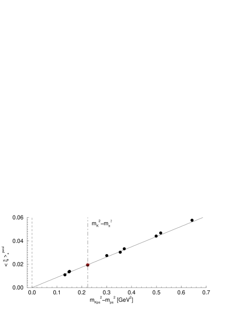
Figure 2: $\langle\xi\rangle_{a}^{\parallel}$ versus $m_{Kps}^{2}-m_{ps}^{2}$ in the $\overline{MS}$ scheme at $\mu=2\,\mbox{GeV}$ for $\beta=5.9$, $\kappa_{sea}=0.1350$, $\vec{p}=\vec{0}$ for various valence quark combinations. A linear fit vanishing when the two valence quark masses are the same is also shown. The red star shows the value when $m_{Kps}^{2}-m_{ps}^{2}=m_{K}^{2}-m_{\pi}^{2}$.

we show $\langle\xi\rangle_{a}^{\parallel}$ versus $m_{Kps}^{2}-m_{ps}^{2}$ together with a one-parameter fit passing through the origin. Also shown (red star) is the value when $m_{Kps}^{2}-m_{ps}^{2}=m_{K}^{2}-m_{\pi}^{2}$. Fig. 3

Figure 3: $\langle\xi\rangle_{a}^{\perp}$ versus $m_{Kps}^{2}-m_{ps}^{2}$. Same notation as for Fig. 2. Note that here we work at finite momentum $|\vec{p}|=2\pi/N_{S}$.

shows the corresponding results for $\langle\xi\rangle_{a}^{\perp}$.

As discussed previously we must now extrapolate $m_{sea}\propto m_{ps}^{2}$ to the chiral limit (the difference between this and $m_{\pi}^{2}$ is negligible). In Fig. 4

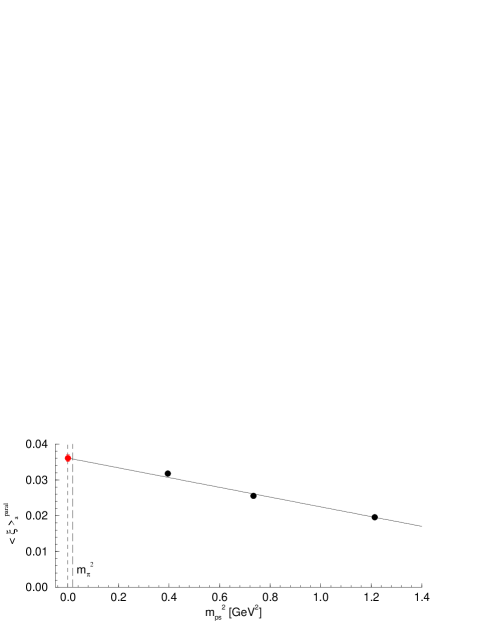
Figure 4: $\langle\xi\rangle_{a}^{\parallel}$ versus $m_{ps}^{2}$ for the three sea quark masses $\kappa_{sea}=0.1350$, $0.1355$ and $0.1359$ (black circles), together with a linear extrapolation to the chiral limit (red circle).

we show this extrapolation for $\langle\xi\rangle_{a}^{\parallel}$ giving an estimate for $\langle\xi\rangle_{K^{*}}^{\parallel}$. In Fig. 5

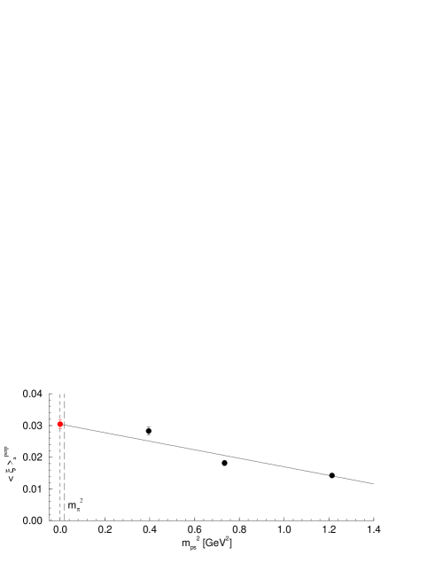
Figure 5: $\langle\xi\rangle_{a}^{\perp}$ versus $m_{ps}^{2}$. Same notation as in Fig. 4.

we show the equivalent picture for $\langle\xi\rangle_{a}^{\perp}$ leading to a value for $\langle\xi\rangle_{K^{*}}^{\perp}$.

This is repeated for other channels and we thus finally arrive at the (preliminary) results

$$\begin{array}[]{lll}\langle\xi\rangle^{\parallel}_{K^{*}}&\approx&0.033(2)(4)\\ \langle\xi\rangle^{\perp}_{K^{*}}&\approx&0.030(2)(8)\\ \end{array}\quad\mbox{or}\quad\begin{array}[]{lll}a_{1K^{*}}^{\parallel}&\approx&0.055(3)(7)\\ a_{1K^{*}}^{\perp}&\approx&0.050(3)(13)\\ \end{array}$$ (13)

(in the $\overline{MS}$-scheme at a scale of $\mu=2\,\mbox{GeV}$) where the first error comes from the spread of channels presently analysed and the second error is an estimation of possible chiral extrapolation error (the fit being repeated dropping one data point). Also any discretisation errors have been ignored.

These are to be compared with the results from sum rule estimates of $a_{1K^{*}}^{\parallel}\approx 0.02(2)$, $a_{1K^{*}}^{\perp}\approx 0.03(3)$ [12] at the same scale, and the limit function $\phi^{asymp}(\xi)$ giving $a_{1K^{*}}^{\parallel,\perp}=0$. Potentially lattice results are more reliable than sum rule estimates and may help in a reconstruction of the vector distribution amplitude.

Our conclusion is that a lattice determination of (moments of) vector DAs is possible. We plan to extend these results to lighter pseudoscalar masses, $\beta=5.40$ (a finer lattice) and to $\langle\xi^{2}\rangle^{\parallel,\perp}$ for both the $K^{*}$ and $\rho$. Further results (including the zero moment decay constants) will appear in [9].

References

- [1] M. Beneke et al., Phys. Rev. Lett. 83, 1914 (1999) [hep-ph/9905312].
- [2] M. Beneke et al., Nucl. Phys. B612, 25 (2001) [hep-ph/0106067].
- [3] Y.-Y. Keum et al., Phys. Rev. D63, 074006 (2001) [hep-ph/0006001].
- [4] C. W Bauer et al., Phys. Rev. D63, 114020 (2001) [hep-ph/0011336].
- [5] P. Ball et al., Phys. Rev. D58, 094016 (1998) [hep-ph/9805422].
- [6] V. Braun et al., Phys. Rev. D74, 074501 (2006) [hep-lat/0606012].
- [7] P. A. Boyle et al., Phys. Lett. B641, 67 (2006) [hep-lat/0607018].
- [8] M. Göckeler et al., Eur. Phys. J. C48, 523 (2006) [hep-lat/0605002].
- [9] M. Göckeler et al., in preparation.
- [10] M. Göckeler et al., Phys. Rev. D71, 114511 (2005) [hep-ph/0410187].
- [11] M. Göckeler et al., in preparation.
- [12] P. Ball et al., JHEP 0703, 069 (2007) [hep-ph/0702100].