Hydrodynamic Simulations of Unevenly Irradiated Jovian Planets

Abstract

We employ a two-dimensional grid-based hydrodynamic model to simulate upper atmospheric dynamics on extrasolar giant planets. The hydrodynamic equations of motion are integrated on a rotating, irradiated sphere using a pseudospectral algorithm. We use a two-frequency two-stream approximation of radiative transfer to model the temperature forcing. This model is well-suited to simulate the dynamics of the atmospheres of planets with high orbital eccentricity that are subject to widely-varying irradiation conditions. We identify six such planets, with eccentricities between $e=0.28$ and $e=0.93$ and semimajor axes ranging from $a=0.0508$ A.U. to $a=0.432$ A.U., as particularly interesting objects for study. For each of these planets, we determine the temperature profile and resulting infrared light curves in the 8-$\mu$m Spitzer bands. Especially notable are the results for HD  80606b, which has the largest eccentricity ($e=0.9321$) of any known planet, and HAT-P-2b, which transits its parent star, so that its physical properties are well-constrained. Despite the variety of orbital parameters, the atmospheric dynamics of these eccentric planets display a number of interesting common properties. In all cases, the atmospheric response is primarily driven by the intense irradiation at periastron. The resulting expansion of heated air produces high-velocity turbulent flow, including long-lived circumpolar vortices. Additionally, a superrotating acoustic front develops on some planets; the strength of this disturbance depends on both the eccentricity and the temperature gradient resulting from uneven heating. The specifics of the resulting infrared light curves depend strongly on the orbital geometry. We show, however, that the variations on HD 80606 b and HAT-P-2b should be readily detectable at 4.5 and 8 $\mu$m using the Spitzer Space Telescope. Indeed, these two objects present the most attractive observational targets of all known high-$e$ exoplanets.

1 Introduction

In July of 1994, the astronomical community was captivated by the collision of comet Shoemaker-Levy 9 and Jupiter. The sudden deposition of energy into the Jovian atmosphere caused a dramatic response on a planetary scale, providing remarkable opportunities for observation and simulation (Harrington & Deming, 2001; Deming & Harrington, 2001) and fostering the development of a deeper understanding of the structure and behavior of gas-giant atmospheres. Within our own solar system, such an occurrence is a one-time event. However, the discovery of extrasolar giant planets on orbits with substantial eccentricity affords the opportunity to study atmospheric dynamics on worlds where the sudden influx of a massive dose of energy occurs on a regular basis. With the advent of Spitzer, direct observation of such planets has become feasible.

The Spitzer telescope has been an unexpectedly useful tool in the study of hot Jupiters, and has already been used to make a number of landmark observations of extrasolar planets. These began with the detections of the secondary eclipses of HD 209458 b (Deming et al., 2005) and TrES-1 (Charbonneau et al., 2005), which confirmed that hot Jupiters have low albedos and day-side effective temperatures of order $T_{\rm eff}\sim 1100\,{\rm K}$. The TrES-1 observations were carried out at 4.5$\mu{\rm m}$ and 8$\mu{\rm m}$, and thus provided an estimate of that planet’s mid-infrared spectral slope. High S/N observations at 16 $\mu{\rm m}$ of the secondary transit of HD 189733 (Deming et al., 2006) produce a similar ($1117\pm 42\,{\rm K}$) day-side temperature.

More recently, Harrington et al. (2006) have detected strong orbital phase-dependent brightness variations for $\upsilon$ And b at 24 $\mu{\rm m}$, which indicate a strong day-night temperature contrast in the far IR, and suggest that heat transfer between the hemispheres is inefficient at the level in the atmosphere that generates the observed $24\mu{\rm m}$ emission. Conversely, Cowan et al. (2007) found no significant orbital phase variations at 8 $\mu{\rm m}$ for 51 Peg b and HD 179949 b, indicating that for those two planets, surface flows are effective at redistributing heat at the level probed by the 8 $\mu{\rm m}$ photosphere. Even more recently, Knutson et al. 2007 have presented results from a continuous 30-hour Spitzer observational campaign on HD 189733. The resulting 8$\mu$m photometric time-series contains extraordinary (part in $10^{-4}$) signal-to-noise and clearly shows phase-dependant flux variations that indicate a day-night temperature contrast of order 200 K. Of particular interest in the Kuntson et al. (2007) time series is a $F/<F>\sim 0.0005$ increase in planetary flux of $\sim 5$hr duration just past the primary transit. This feature can be interpreted as arising from a hotspot near the dawn terminator of the planet.

In addition to providing infrared photometric time-series data, the Spitzer Space Telescope can also be used to obtain mid-infrared spectra of extrasolar planets. This has been done for the transiting planets HD 209458b (Richardson et al. 2007) and HD 189733b (Grillmair et al. 2007). In both cases, spectra in the 7-14$\mu$m range were obtained by subtracting the stellar spectrum measured during secondary eclipse from the combined star+planet spectrum obtained just outside eclipse. Model atmospheres of extrasolar planets under strong insolation conditions (e.g. Sudarsky, Burrows & Hubeny 2003, Marley et al. 2006) predict that ${\rm H_{2}O}$ absorption features would be prominent within the observed spectral range. Remarkably, however, neither planet displayed the predicted signature. This null result can be interpreted in several ways. First, it is possible that the atmospheres are dry, perhaps because available oxygen is sequestered in CO. This interpretation, however would require both planets to have unexpectedly large C to O ratios. Alternately, the effectively featureless spectrum could arise from a very clear atmosphere with an isothermal P-T profile down to large optical depth (Fortney et al., 2006). This interpretation is favored by the fact that the hot Jupiters have extremely low albedos (Rowe et al. 2006). As a third possibility, Harrington et al. (2007) suggest that HD 209458b may be displaying line emission at 10$\mu$m. They interpret these features as possibly arising from silicate clouds. Any such clouds, however, would need to be highly non-reflective in order to be consistent with the low optical albedo.

At present, the existing observational results present an incomplete and somewhat contradictory overall picture. It is not understood how the wind vectors and temperature distributions on the observed planets behave as a function of pressure depth, and planetary longitude and latitude. Most importantly, the effective radiative time constant in the atmospheres of short-period planets remains unmeasured, and as a result, dynamical calculations of the expected planet-wide flow patterns (Cho et al. 2003, Cooper & Showman 2005, Burkert et al. 2005, Fortney et al. 2006, Langton & Laughlin 2007, Dobbs-Dixon & Lin 2007) have come to no consensus regarding how the surface flow should appear. The lack of agreement between the models stems in large part from the paucity of unambiguous measurements of the basic thermal structure of the atmospheres of short-period planets. Essentially, the problem comes down to the fact that the planets that have been observed so far have had their spin periods tidally synchronized to their orbits, so that each spot on the substellar surface sees a constant illumination from the parent star. The resulting flow pattern will therefore likely be in steady state, and the temperature distribution across the planetary surface will depend on both the radiative timescale as well as the windspeeds at optical depth unity.

In this paper, we discuss our modeling program for determining the hydrodynamic flows on the surfaces of planets traveling on significantly eccentric orbits. Such planets are not spin-synchronous. Tidal effects cause the rotation rate to approximate the orbital angular velocity at periastron; the rotation is therefore pseudo-synchronous and the spin period is a sensitive function of the eccentricity (Hut, 1981). In contrast to the typical spin-synchronous hot Jupiter, on which one hemisphere is perpetually illuminated while the other receives no insolation, the entire surface of an eccentric planet receives radiation. Pseudo-synchronization does, however ensure that a single hemisphere receives the preponderance of the illumination during the periastron passage. Additionally, the intensity of the radiation received varies strongly over the course of an orbit. The insolation of planets on eccentric orbits therefore exhibits significant time variation.

To our knowledge, other modeling efforts to date have focused exclusively on exoplanets that are in tidally synchronized orbits with a permanent day-night side asymmetry and essentially steady state irradiation conditions. With such bodies, it is difficult to disentangle the contributing effects of the effective radiative time constant in the planetary atmosphere, and the hydrodynamic flow velocities on the surface. In this paper, we propose that these ambiguities can be resolved by observing planets that have eccentric orbits, and which hence show different hemispheres (or partial hemispheres) to the star, and which experience a highly variable total insolation. We identify the highly eccentric planet HD 80606 b and the transiting planet HAT-P-2 b (Bakos et al., 2007) as being a prime targets for such observations. We propose that by monitoring these planets during their periastron passages, we can improve our overall understanding of the atmospheric properties of hot Jupiters. The planet-wide response to the rapid increase in stellar radiation will be readily observable in the 4.5$\mu{\rm m}$ and 8$\mu{\rm m}$ bands, and will provide a direct simultaneous measurement of the radiative time constant at two separate levels in the atmosphere.

The plan for this paper is as follows. In §2, we describe our numerical model as applied to extrasolar planets. In §3, we discuss the characteristics of the six planets considered in this paper, as well as relevant stellar properties of their parent stars. In §4, we present the results of this model as applied to these planets. In §5, we discuss the observational consequences of these results, in particular concentrating on the infrared light curves in the 8 micron Spitzer band. We show that in general, the periastron passage produces a distinct flux peak, and that the shape of the overall curve can be used to constrain planetary characteristics such as rotation rate and atmospheric radiative time constant. We conclude in §6.

2 Numerical Model

We begin with the primitive hydrodynamic equations of motion in two dimensions, assuming hydrostatic equilibrium:

$$\frac{\partial\rho}{\partial t} = -\mathbf{v}\cdot\nabla\rho-\rho\nabla\cdot\mathbf{v}$$ (1)

$$\frac{\partial\mathbf{v}}{\partial t} = -\mathbf{v}\cdot\nabla\mathbf{v}-\frac{1}{\rho}\nabla p$$ (2)

$$\frac{\partial}{\partial t}\left(\frac{e}{\rho}\right) = -\mathbf{v}\cdot\nabla\left(\frac{e}{\rho}\right)-\frac{p}{\rho}\nabla\cdot\mathbf{v}.$$ (3)

We use the equation of state for an ideal gas: $p=(\gamma-1)e=\rho RT$, where $R$ is the specific gas constant and the adiabatic constant $\gamma=1.4$ for a diatomic gas. (We actually use a value of $\gamma=1.389$, appropriate for molecular hydrogen at 900 K.) Setting the specific heat capacity to $C_{V}=R/(\gamma-1)$, we can substitute

$$T=\frac{1}{C_{V}}\frac{e}{\rho}$$ (4)

into equation (3) to obtain the hydrodynamic equations in terms of the dynamical variables $T,\mathbf{v},$ and $\rho$:

$$\frac{\partial T}{\partial t} = -\mathbf{v}\cdot\nabla T-(\gamma-1)T\nabla\cdot\mathbf{v}$$ (5)

$$\frac{\partial\mathbf{v}}{\partial t} = -\mathbf{v}\cdot\nabla\mathbf{v}-\frac{RT}{\rho}\nabla\rho-R\nabla T$$ (6)

$$\frac{\partial\rho}{\partial t} = -\mathbf{v}\cdot\nabla\rho-\rho\nabla\cdot\mathbf{v}.$$ (7)

In order to obtain a model appropriate to planetary atmospheric flows, we add a thermal forcing term to (5) and a Coriolis term to (6), obtaining the equations of hydrodynamic motion on an irradiated, rotating sphere:

$$\frac{\partial T}{\partial t} = -\mathbf{v}\cdot\nabla T-(\gamma-1)T\nabla\cdot\mathbf{v}+f_{rad}$$ (8)

$$\frac{\partial\mathbf{v}}{\partial t} = -\mathbf{v}\cdot\nabla\mathbf{v}-\frac{RT}{\rho}\nabla\rho-R\nabla T-2\Omega_{rot}\sin\theta(\hat{n}\times\mathbf{v})$$ (9)

$$\frac{\partial\rho}{\partial t} = -\mathbf{v}\cdot\nabla\rho-\rho\nabla\cdot\mathbf{v},$$ (10)

where $f_{rad}$ gives the thermal forcing, $\Omega_{rot}$ is the angular frequency of the planet’s rotation, $\theta$ is the latitude, and $\hat{n}$ is a unit vector normal to the planet’s surface.

We calculate $f_{rad}$ using a one-layer, two-frequency radiative transfer scheme. For hot Jupiters, the bulk of the energy input occurs near the peak of the stellar spectrum in the visible $\lambda_{\rm max}\sim 2.73/T_{\star}\sim 0.5\mu$. Energy balance, on the other hand, is maintained via thermal re-radiation in the infrared $\lambda_{\rm max}\sim 2.73/T_{\rm pl}\sim 3\mu$. The separation of the corresponding blackbody distributions motivates our use of a two-frequency scheme. We take the mean opacity for incident stellar radiation to be $k_{1}$, while the mean opacity for outgoing long-wave radiation is $k_{2}$. In this greatly simplified model, a thin layer of the atmosphere with thickness $dz$ and at a pressure depth $p$ will absorb a flux equal to

$$dF=\left(\frac{k_{1}F_{*}(p)}{\cos\alpha}+k_{2}\sigma T_{n}^{4}-k_{2}\sigma T^{4}\right)\rho\phantom{i}dz,$$ (11)

where $F_{*}(p)$ is the incident stellar flux at a pressure depth $p$, $\alpha$ is the zenith angle of the star, $T_{n}$ is the temperature of the layer being modeled in the absence of solar heating, and $\sigma=5.67\cdot 10^{-8}$ W m^-2 K^-4 is the Stefan-Boltzman constant. $T_{n}$ is the result of the combination of the intrinsic planetary flux due to tidal heating and the heating supplied by the atmosphere at high optical depth, and is calculated using a one-dimensional two-stream approximation to radiative transfer similar to that used in Iro et al. (2005). The details of the $T_{n}$ calculation are discussed in greater detail in §3.

Energy conservation requires that $dF=\rho C_{p}f_{rad}dz$, so the thermal forcing must be

$$f_{rad}=\left(\frac{1}{C_{p}}\right)\left(\frac{k_{1}F_{*}(p)}{\cos\alpha}+k_{2}\sigma T_{n}^{4}-k_{2}\sigma T^{4}\right).$$ (12)

We may approximate $F_{*}(p)$ by ignoring the variation in $k_{1}$ with temperature and pressure; this gives

$$F_{*}(p)=F_{*}(0)e^{-\frac{k_{1}p}{g\cos\alpha}}.$$ (13)

But $F_{*}(0)$ is simply the flux at the top of the atmosphere, which is

$$F_{*}(0)=(1-A)\left(\frac{L_{*}}{4\pi a^{2}}\right)\cos\alpha,$$ (14)

where $A$ is the Bond Albedo, $L_{*}$ is the stellar luminosity, and $a=a(t)$ is the time-dependent distance between the star and the planet. Then the thermal forcing is

$$f_{rad}=\left(\frac{1}{C_{p}}\right)\left(k_{1}(1-A)\left(\frac{L_{*}}{4\pi a^{2}}\right)e^{-\frac{k_{1}p}{g\cos\alpha}}+k_{2}\sigma T_{n}^{4}-k_{2}\sigma T^{4}\right).$$ (15)

With a little bit of algebraic manipulation, this can be placed in a more transparent form:

$$f_{rad}=\beta\left(T_{eq}^{4}-T^{4}\right),$$ (16)

where $\beta=\sigma k_{2}/C_{p}$ and the equilibrium temperature $T_{eq}$ follows

$$T_{eq}^{4}=\left(\frac{k_{1}}{k_{2}}\right)T_{ss}^{4}x^{\sec\alpha}+T_{n}^{4},$$ (17)

with $\sigma T_{ss}^{4}=(1-A)L_{*}/(4\pi a^{2})$ and $x=\exp(-k_{1}p/g)$. The forcing that results from this scheme strongly depends on the choice of $k_{1}$, $k_{2}$, and $p$. Motivated by many-layer radiative models of HD 209458 b (Iro et al., 2005), we choose $k_{1}=2\cdot 10^{-4}$ m² kg^-1, $k_{2}=4\cdot 10^{-4}$ m² kg^-1, and $p=250(g/10$ m s${}^{-2})$ mbar, where $g$ is the acceleration due to gravity at the planet’s surface.

While we believe this model represents an improvement over earlier work, it is nevertheless unable to account for a number of potentially important effects. Two-dimensional hydrodynamics obviously cannot account for vertical atmospheric flows. Since the infrared photosphere is well inside the radiative zone for the planets under consideration, it is likely that convective effects are negligible. However, the inability of the model to account for vertical expansion under heating could cause some error.

In our radiative model, we make a number of simplifications are likely to cause discrepancy between our predictions and observations. We ignore the variation of opacities with temperature and pressure, which is known to be significant. We furthermore do not consider the variation in opacity with wavelength within the infrared regime; this implies that, for example, the 24-micron photosphere and the 3-micron photosphere occur at the same pressure level. The planets in our simulations experience large temperature variations, which may lead to the formation and dispersal of different cloud species (Sudarsky, Burrows & Hubeny, 2003; Marley et al., 2007). We do not, however, include the formation of clouds in our model.

Despite these shortcomings, this model represents a significant improvement over earlier simulations in a number of areas. Shallow water models can achieve high resolution, but also have difficulty modeling certain qualitative aspects of the flow; temperature waves redistribute heat far more efficiently than is realistic. Since our code employs fully compressible hydrodynamics, we are able to simulate heat transfer within atmospheric flows with greater realism than is possible using incompressible shallow-water dynamics.

Furthermore, our radiative scheme provides a more realistic model of the thermal forcing than the Newtonian relaxation employed in earlier hydrodynamic simulations (Cho et al., 2003; Cooper & Showman, 2005; Langton & Laughlin, 2007). While Newtonian relaxation is a reasonable approximation when the temperature is close to the equilibrium temperature, it becomes dramatically less accurate as the temperature perturbations grow larger. In the forcing regimes expected on extrasolar planets, the Newtonian approximation can overestimate the actual rate of temperature change by as much as a factor of 3. Our radiative model therefore allows us to treat the stellar heating more accurately than previous simulations; this is particularly important in cases where the thermal forcing varies significantly with time, either due to non-synchronous rotation or to a highly eccentric orbit.

Equations (8) through (10) are numerically integrated using the vector spherical harmonic transform method (Adams & Swarztrauber, 1999). We use a longitude-latitude grid with T171 resolution ($512\times 257$), sufficiently fine to resolve the details of turbulent flow. Numerical stability is maintained using fourth-order hyperviscosity (Polvani et al., 2004), which prevents the spurious addition of energy at small scales. This is accomplished by adding a term of the form $B\nabla^{4}\phi$ to each of the time-evolution equations, where $\phi$ is the evolving quantity. To minimize the effect of this numerical dissipation on the flow evolution, $B$ is generally chosen to be as small as possible, while still preventing unphysical spectral ringing or numerical instability. In general, this requires $B\sim 10^{-12}a^{4},$ where $a$ is the planetary radius. This results in a decrease in $\phi$ of $\sim$ 5 % per time step at the smallest spectral scales; with such strongly-varying heating, anything less allows pernicious behavior.

The planetary atmosphere is initially at constant pressure, isothermal, and nearly at rest, with only a small random initial flow to break the unphysical north-south symmetry. Since the resulting flow is often turbulent, the specific evolution of the dynamical variables changes from one run to the next. Nevertheless, the qualitative properties of the flow are not altered by small changes to the initial wind flow. The initial temperature is chosen so that it approximately equals the average equilibrium temperature; this prevents the initial thermal forcing from inducing the large winds that result if, for example, the initial temperature is $T_{n}$ (Cooper & Showman, 2005). While other groups have obtained supersonic flow, these seem to occur in simulations where either the night-side equilibrium temperature is unusually low (Dobbs-Dixon & Lin, 2007) or the planet is initially cold (Cooper & Showman, 2005). The first situation maintains an artificially high equilibrium temperature gradient; the second greatly amplifies the effect of the initial heating, particularly if the stellar heating is not introduced gradually. In either case, there is good reason to believe that the actual wind speeds may be subsonic. The planet is allowed to evolve from its initial state until a dynamical equilibrium is reached – typically $\sim 100$ days – and then the temperature, density, wind velocity, and relative vorticity are recorded.

3 Planetary Characteristics

Our code requires a number of planetary characteristics as input parameters. The mass and radius of the planet must be specified in order to determine the surface gravity and therefore the appropriate pressure at the infrared photosphere. The orbital period, semi-major axis, and eccentricity of the planet’s orbit are required to calculate the time-dependent irradiation conditions. Additionally, the longitude of periastron is needed to produce the light curves. With the exception of the planetary radius, all of this information can be found in Butler et al. (2006). The radii are determined using the planetary structure model of Bodenheimer et al. (2003). To determine correctly the mass and the light curve, it is also necessary to know the orbital inclination. In general, however, this can be constrained only in the case of a transit. Nevertheless, inclinations close to $90^{\circ}$ are more probable. We therefore take the minimum value of the planetary masses; that is, $\sin i=1$. The effect of the planetary mass enters the simulation primarily by determining the magnitude of the gravitational acceleration at the planetary surface. Test runs of our model varying gravity by up to a factor of 10 produce little change in the resulting flow patterns. Since a two-dimensional model of a radiative atmosphere necessarily assumes hydrostatic balance and vertical stratification, the small impact of gravity is not surprising. In any case, it is clear that in our model, the actual mass of the planet is of negligible importance; the minimum mass assumption therefore introduces no significant inaccuracies.

The planet’s rotation rate is also an important parameter, necessary to determine both the substellar point and the strength of the Coriolis effect. In the case of a close-in circular orbit, planetary rotation is expected to be synchronous, so that the orbital period and the rotation period are identical. If the orbit is even slightly eccentric, however, spin-synchronization is broken. Tidal effects are strongest at periastron, and therefore the preferred rotation rate is approximately the angular frequency at periastron. The result is a state of spin pseudo-synchronization, wherein the rotation rate is a well-defined function of the eccentricity (Hut, 1981):

$$\tau_{rot}=\tau_{orb}\left(\frac{(1+3e^{2}+\frac{3}{8}e^{4})(1-e^{2})^{3/2}}{1+\frac{15}{2}e^{2}+\frac{45}{8}e^{4}+\frac{5}{16}e^{6}}\right).$$ (18)

Recently, Ivanov & Papaloizou (2007) have advanced an alternate theory for spin-synchronization which predicts that planets in highly eccentric orbits will have spin angular velocities that are close to 1.55 times the circular orbit angular velocity at periastron. As will be clear from our simulations in this paper, long-duration observations with the Spitzer Space telescope can in principle be used to distinguish between the two models for spin pseudo-synchronization. In this initial work, however, we adopt the Hut (1981) theory for our assumed planetary spin rates.

In addition to the planet’s physical and orbital characteristics, we also must determine the equilibrium night-side temperature, $T_{n}$ at the simulation pressure depth $p=250(g/10$ m s${}^{-2})$ mbar. This represents a combination of the planet’s intrinsic luminosity due to tidal dissipation and gravitational contraction and the redistribution of incident stellar radiation at high optical depths. With the exception of HD 80606 b, which is characterized by an extremely high tidal luminosity and relatively low average insolation, the night side temperatures of the planets here considered are largely determined by the incident radiation.

We determine $T_{n}$ using a one-dimensional plane-parallel two-stream algorithm with $N=100$ vertical zones. In keeping with the radiative model described in §2, we consider only two frequencies and neglect the variation in opacities with temperature and pressure. The results of these calculations are therefore not precise, but are likely to give reasonable estimates of the atmospheric temperature in the absence of direct stellar heating. At the upper boundary, we impose a downward flux equal to the time-averaged stellar radiation

$$<F_{\downarrow}>=\frac{L_{*}}{16\pi}\left<\frac{1}{r^{2}}\right>=\frac{L_{*}}{16\pi a^{2}}\frac{1}{\sqrt{1-e^{2}}}.$$ (19)

At the lower boundary, which we set at $p=5.0(g/10$m s^-2) bar, we require a net upward flux consistent with the planet’s intrinsic luminosity. We then allow the atmosphere to come to radiative equilibrium, thereby determining the temperature at the base of the atmosphere. We then maintain the lower boundary at this temperature, and recalculate the equilibrium temperature at each layer in the absence of stellar radiation. This quantifies the response of the upper atmosphere to heating by high-temperature interior layers. We take $T_{n}$ to be the atmospheric temperature at the layer corresponding to the pressure depth used in our simulations. The planetary parameters, including $T_{n}$ and $\tau_{rot}$, are summarized in Table 1.

Finally, the characteristics of the parent star are necessary to determine the magnitude of the incident stellar radiation, as well as the relative planet-star infrared flux as a function of wavelength. From Butler et al. (2006), we obtain the stellar mass, radius, temperature, and luminosity, although our model only requires the temperature and luminosity. These data are compiled in Table 2.

We wish to focus particular attention on two planets: HD 80606 b and HAT-P-2 b. With $e>0.9$, HD 80606 b is the most eccentric planet known by a significant margin. Because both the rotation rate and the characteristics of the periastron passage depend strongly on the eccentricity, it is especially important to obtain an accurate value. Using both the 55 radial velocities published in support of the initial detection (Naef et al., 2001) and a further 46 radial velocities published by Butler et al. (2006), we obtain best-fit values for the relevant planetary characteristics: the orbital period $\tau_{orb}=111.4298\pm 0.0032{\rm d}$, the eccentricity $e=0.9321\pm 0.0023$, and the longitude of periastron $\varpi=300.264^{\circ}\pm 0.35^{\circ}$.

HD 80606’s mass is estimated to lie between 0.9 and 1.1 $M_{\odot}$ (Naef et al. 2001, Butler et al. 2006). Adopting $M=1M_{\odot}$, we derive $M_{\rm pl}\sin(i)=4.18\,M_{\rm Jup}$. Our planetary models (Laughlin et al. 2005) predict a radius of $1.10\pm 0.02\,R_{\rm Jup}$. The uncertainty in $R_{\rm pl}$ is small because the planet lies in the mass regime where the radius is an extremely weak function of the mass. Furthermore, the planet is sufficiently massive enough that while it experiences considerable internal heating associated with its strong tidal dissipation, the heating (which we estimate below to be $L\sim 10^{28}$ ergs) is expected to have a negligible impact on the planet’s physical radius (Gu, Bodenheimer, & Lin 2004). The well-determined radius is important because it largely eliminates an unknown free parameter when we model the hydrodynamic response.

Because of the extreme eccentricity and relatively large semi-major axis of HD 80606 b’s orbit, tidal heating becomes a significant contribution to the overall planetary temperature. Wu & Murray (2003) posit that HD 80606 b’s large eccentricity was initially produced by resonant interaction with HD 80607, a binary companion to HD 80606 with a wide separation $\sim 1000$ A.U. Wu and Murray show that if HD 80606 b initially formed in an $a_{\rm init}=5$ A.U. orbit that was highly inclined to the binary plane, then the Kozai resonance (Kozai, 1962) would have quickly driven the planet’s eccentricity to $e\sim 0.993$. In the Wu-Murray theory, successive cycles of high eccentricity and attendant tidal orbital decay acted to decrease the semi-major axis. Once $a$ dropped below $\sim 3$ A.U., the Kozai resonance was destroyed by general relativistic precession. Over the last few Gyr, the planet has undergone continuous tidal dissipation, which has decreased $a$ and $e$ to their current values. By considering the amount of orbital energy lost over this time period, Wu & Murray arrive at a tidal luminosity $L_{tid}\approx 10^{28}$ erg. For the sake of comparison, the average incident stellar radiation absorbed by the planet is $L_{rad}=3\cdot 10^{27}$ ergs. It is likely, therefore, that the dominant contribution to $T_{n}$ on HD 80606 b arises from eccentricity tides rather than convective redistribution of incident radiation.

HAT-P-2 b also deserves special consideration. It was discovered via the transit method by Bakos et al. (2007). Because it transits its parent star, its mass $M=8.17M_{J}\pm 0.72M_{J}$ and radius $R=1.18R_{J}\pm 0.16R_{J}$ are well-constrained. In particular, the $\sin i$ degeneracy is broken, since the inclination $i=90.0^{\circ}\pm 1^{\circ}$ has been directly measured. Furthermore, we have direct determination of the radius; this is particularly valuable given the divergence of observed radii from models in a number of cases (Sato et al., 2005; Bodenheimer et al., 2003; Laughlin et al., 2005). HAT-P-2b orbits a bright (V=8.7) star with a period of 5.63 d; furthermore, its orbital geometry ($\varpi=185^{\circ}$), ensures that the periastron passage is midway between the primary and secondary transits and that all three events are observable within a 36-hour period. HAT-P-2b is therefore uniquely well-suited for observation.

4 Dynamical Evolution of the Planetary Atmospheres

Representative atmospheric temperature distributions for each planet considered in this paper, with the exception of HD 37605 b, are presented in Figure 1. Our simulations demonstrate that eccentric exoplanets exhibit great diversity in their atmospheric flow patterns and temperature distributions, with eccentricity, periastron distance, orbital period, and stellar luminosity all playing important roles. Nevertheless, all of the planets here considered display significant subsolar heating at periastron, with temperature increases ranging from 300 K to 700 K. Planets with high eccentricities and strong periastron heating may also develop high-amplitude superrotating acoustic waves in response to a high temperature gradient near the eastern terminator. Due to the temperature dependence of the sound speed, the acoustic waves emitted inside hotter regions overtake those emitted at the cooler terminator, causing a region of very high density only a few zones wide. This “acoustic compression” produces a front propogating eastward, maintaining its intensity as it is repeatedly focused by reflections off of the cooler, denser polar air.

It is not immediately obvious why our model predicts the formation of these acoustic disturbances on some planets but not on others. The orbit of HD 37605 b is considerably more eccentric ($e=0.737$) than that of HAT-P-2 b ($e=0.507$), yet HAT-P-2 b exhibits a clearly defined acoustic disturbance which is absent from HD 37605 b. The periastron flux received by HD 80606 b is smaller than that received by HD 118203 b and HD 185269 b, which orbit more luminous stars. Furthermore, HD 80606 b has a comparatively small temperature variation and correspondingly slower wind speeds. Yet the stellar heating received by HD 80606 b generates large-amplitude acoustic waves, whereas the flow on HD 118203 b and HD 185269 is primarily vortical, with no large-scale acoustic fronts. While we have not investigated this issue in detail, our calculation of predicted light curves suggests that the subsolar heating rate at periastron is the determinating factor in the formation of a strong acoustic front. Sufficiently rapid heating at periastron produces a large local temperature gradient which, as described above, generates a region of high density and pressure which then propagates acoustically; slower periastron heating causes a shallower temperature gradient, less acoustic compression, and therefore any acoustic waves are much lower amplitude.

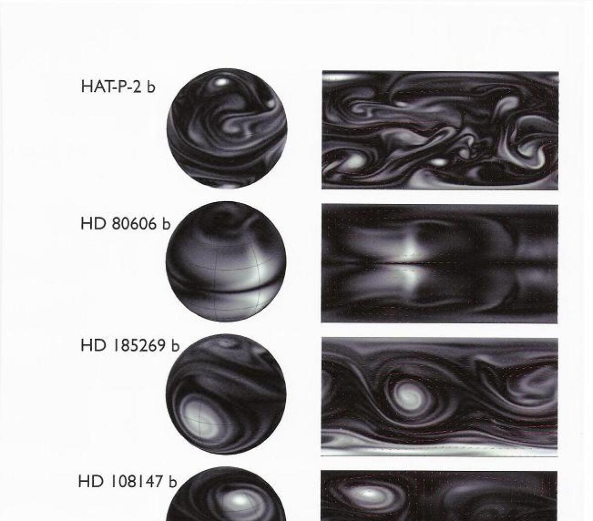
Figure 2: Relative vorticity distributions and wind flow patterns for each planet modeled. The globes on the left show a three-dimensional representation of the (absolute value of) relative vorticity. The plots on the right show an equirectangular plot of the wind velocity field superimposed on the vorticity distribution. The flow pattern is taken at the same time as the temperature distribution in Figure 1. The maximum wind speeds in each plot are as follows: HAT-P-2 b: 1050 m s^-1; HD 80606 b: 380 m s^-1; HD 185269 b: 1410 m s^-1; HD 108147 b: 930 m s^-1; HD 118203 b: 1100 m s^-1. The maximum relative vorticities are: HAT-P-2 b: 1.1$\cdot 10^{-4}$ s^-1; HD 80606 b: 1.8$\cdot 10^{-5}$ s^-1; HD 185269 b: 1.2$\cdot 10^{-4}$ s^-1; HD 108147 b: 1.3$\cdot 10^{-4}$ s^-1; HD 118203 b: 1.1$\cdot 10^{-4}$ s^-1. (Note that the relative vorticity at a particular point corresponds to the angular frequency of rotation of a paddlewheel placed in the flow at that point.)

In order to elucidate the dynamics of the flow itself, we show in Figure 2 the vorticity distribution on five of the six planets modeled; again, we omit the results for HD 37605 b. The distributions are shown at the same time and, in the case of the globe view, from the same vantage point as in Figure 1. A quiver plot superimposed on the equirectangular map shows the direction and relative wind speed of the flow itself.

From both the temperature and vorticity distributions, it is clear that with the exception of HD 80606 b, each planet exhibits large-scale turbulent eddies. Given the extreme eccentricity of this planet’s orbit, this is perhaps surprising. However, the lack of turbulence can be explained by the relatively low temperature contrast (which we take to be $T_{max}-T_{min}$, where $T_{max}$ and $T_{min}$ are respectively the global maximum and minimum temperatures at a given moment) seen on HD 80606 b. While this temperature contrast reaches 500 K momentarily, the rapid periastron passage prevents the planet from receiving enough heat to sustain these temperature differences; within 72 hours of periastron, the temperature difference has fallen to 250 K, continuing to drop after that. In comparison, the temperature difference on HAT-P-2b exceeds 1100 K at periastron, with an average value of 540 K. While we have not run a sufficient number of simulations to be precise, it appears that sustained temperature differences greater than 250 to 300 K are required to generate large-scale vortical structure. It is important that this temperature contrast be prolonged; while brief exposure to a large temperature gradient induces divergent flow, it appears that it takes some time for the Coriolis force to produce a large and persistent rotational component.

It is interesting to note here the significance of $T_{n}.$ For a particular amount of stellar heating, as $T_{n}$ increases, the induced temperature gradient becomes smaller, and both wind speed and turbulence decrease. We find, for example, that a lower value of tidal heating on HD 80606 b, leading to $T_{n}=400$ K provides a sufficiently cool background that HD 80606 b develops a temperature difference which remains over 300 K for 10 d after periastron, thereby producing turbulent flow comparable to the other planets. Similiarly, a test run on HD 118203 b with $T_{n}=1960$ K (a change with absolutely no physical justification!) reduced the maximum temperature contrast on that planet to 200 K, stifling the development of the hemisphere-scale vortices so prominent in our earlier simulation.

The intrinsic temperature of the planet then rises to a question of first-order importance. While the infrared observations resulting from the evolution of a particular temperature distribution are not sensitive to small-scale differences in the flow, a global-scale qualitative shift from laminar to turbulent flow fundamentally alters the temperature distribution, with possibly significant observational impact. Given the importance of tidal heating in determining the intrinsic luminosity, in addition to the unsuitability of an equilibrium model of tides to predicting the tidal dissipation on these highly dynamic objects, further development of a dynamical theory of tides seems to be a promising field for future investigation.

5 Infrared Emission Curves

The flux $F_{\lambda}$ emitted by a planet with some temperature distribution $T(\phi,\theta)$ between wavelengths $\lambda$ and $\lambda+d\lambda$ is

$$F_{\lambda}=\int B_{\lambda}(T)\cos\alpha\cos\theta r_{p}^{2}d\theta d\phi d\lambda,$$ (20)

where $B_{\lambda}(T)$ is the Planck function for emission at a wavelength of $\lambda$ by a blackbody at temperature $T$, and $\alpha$ is the angle between the surface normal and a vector directed from the planet to the observer. The integral is performed over the hemisphere visible to the observer, that is, where $\cos\alpha>0$. In the case of a grid-based model, this can be discretized as follows:

$$F_{\lambda}=\sum\bar{B}_{\lambda}(T)\cos\alpha\cos\theta r_{p}\Delta\theta\Delta\phi,$$ (21)

where

$$\bar{B}_{\lambda}(T)=\int B_{\lambda}(T)d\lambda.$$ (22)

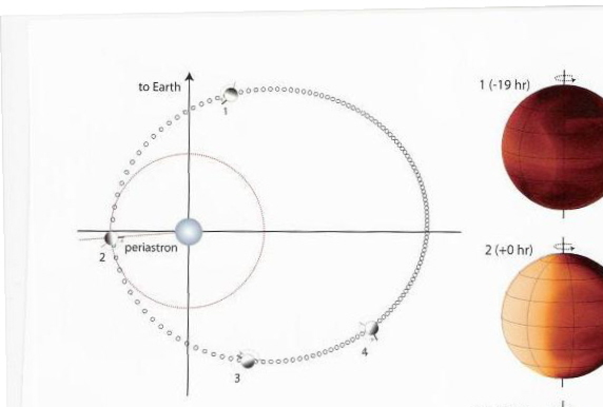
Figure 4: A detailed representation of the results of the HAT-P-2 b simulation. The small points on the orbital diagram show the position of the planet at one-hour intervals; the larger globes (labeled 1 through 4) show the position of the planet at times $t=-19\rm{h},0\rm{h},+19\rm{h},+38\rm{h}$ relative to periastron. The black poles on these globes show the rotation of a stationary point on the planetary surface; the gray poles indicate the amount of rotation that has occurred over a 19-hour period. The hemispheric plots on the right show the atmospheric temperature distribution at the corresponding times. The light curve shows the planet’s infrared emission in the 8 $\mu$m band from 25 h before to 50 h after periastron.

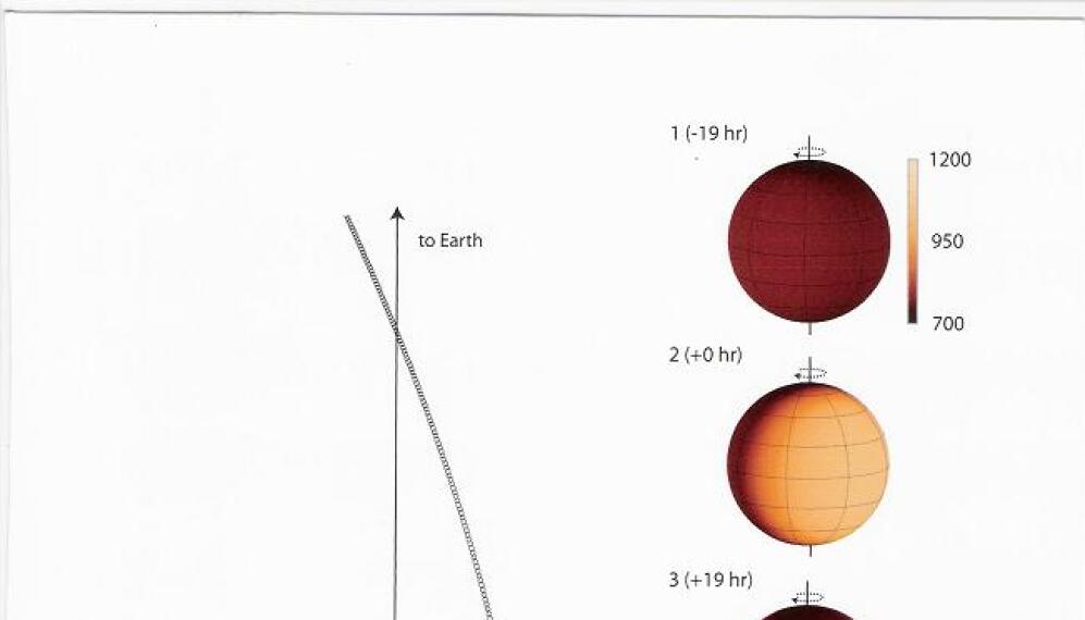
Figure 5: A detailed representation of the results of the HD 80606 b simulation. The small points on the orbital diagram show the position of the planet at one-hour intervals; the larger globes (labeled 1 through 4) show the position of the planet at times $t=-19\rm{h},0\rm{h},+19\rm{h},+38\rm{h}$ relative to periastron. The black poles on these globes show the rotation of a stationary point on the planetary surface; the gray poles indicate the amount of rotation that has occurred over a 19-hour period. The hemispheric plots on the right show the atmospheric temperature distribution at the corresponding times. The light curves show the planet’s infrared emission in the 8 $\mu$m band from 25 h before to 50 h after periastron. The red curve corresponds to an orbital inclination of $i=90^{\circ}$ (in which the orbit is being viewed edge-on), the purple to $i=60^{\circ}$, the blue to $i=30^{\circ}$, and the black to $i=0^{\circ}$.

We apply equation (21) to the temperature distributions considered in §4 to produce planetary infrared light curves; the results are shown in Table 3 and Figures 3, 4, and 5. In Figures 4 and 5, the small points on the orbital diagram show the position of the planet at one-hour intervals; the larger globes (labeled 1 through 4) show the position of the planet at times $t=-19\rm{h},0\rm{h},+19\rm{h},+38\rm{h}$ relative to periastron. The black poles on these globes show the rotation of a stationary point on the planetary surface; the gray poles indicate the amount of rotation that has occurred over a 19-hour period. The hemispheric plots in the right portion of the figures show the atmospheric temperature distribution at the corresponding times. The light curves shows the planets’ infrared emission in the 8 $\mu$m band from 25 h before to 50 h after periastron.

These light curves vary widely in their shape, range, and time scales, as is expected given the range of irradiation conditions and orbital parameters. All show some degree of interesting structure; none can be well-fit by the simple sinusoidal shape predicted by earlier models (Cooper & Showman, 2005; Langton & Laughlin, 2007). We note two particularly promising candidates for observation. HD 80606 b, which reaches a peak flux $F/F_{*}=8.0\cdot 10^{-4}$ in the 8-$\mu$m band, will be observed by the Spitzer Space Telescope during its periastron passage in November 2007. HAT-P-2 b, which exhibits even larger flux variation over the course of its orbit, provides an equally attractive target for observation. The flux variations for both objects are sufficiently large to be comfortably resolved by Spitzer (Charbonneau et al., 2005; Harrington et al., 2006, 2007). The other four planets, HD 37605 b, HD 108147 b, HD 118203 b, and HD 185269 b, present significantly greater observational challenges. However, it is not infeasible that the light curve variations on some of the brighter planets – HD 118203 b and HD 108147 b – could be resolved with sufficiently long integration times.

6 Conclusion

The advent of the Spitzer Space Telescope and the discovery of short-period planets on significantly eccentric orbits has presented astronomers with the opportunity to observe time-dependent weather patterns on extrasolar planets. Giant planets on eccentric orbits that experience strong variations in insolation have the potential to tell us a great deal about the structure, dynamics and chemistry of Jovian-like atmospheres. Eccentric planets can be profitably compared with short period planets on spin-synchronous circular orbits that are likely to have largely steady-state patterns of surface flow, and which are currently being observed with Spitzer.

Furthermore, when eccentricities are extreme – as in the case of HD 80606 b – we are afforded the ability to directly observe planets that spend the bulk of their orbit in a region where the radiation environment is similar to that experienced on Earth. With current instruments, such planets would be completely beyond the possibility of direct observation.

Eccentric planets also have the best potential to give us an understanding of the dissipative mechanisms at work in planetary interiors. A planet such as HAT-P-2 b should be generating a very significant luminosity as a result of the strongly time-dependent tidal force on the planet. By observing the depth of the primary transit in the infrared, one can get a direct measurement of the planetary effective temperature, which can then be used to infer the amount of dissipation within the planet, and to put interesting constraints on the tidal quality factor, $Q$ associated with dynamical (as opposed to equilibrium) tides.

To take a first step toward understanding what to expect from the infrared light curves of short-period eccentric planets, we have created a two-dimensional hydrodynamic model with radiative forcing appropriate to the time-varying illumination received for a specified orbit. Our model handles radiation transfer in an approximate, but hopefully qualitatively correct manner by separating the transport of optical and IR radiation. We apply this model to six known giant planets on eccentric orbits with $e\gtrsim 0.3$. The irradiation intensity on these planets varies by a factor of three for the least eccentric planets up to a factor of 800 for HD 80606b. The effect of this tremendous variability on atmospheric flows is profound; the dominant feature in the evolution of each atmosphere studied is the subsolar heating through the perastron passage, with the subsequent flow being primarily driven by this dramatic forcing. For each planet, we find significant spatial and temporal variability in the state of the atmosphere, with turbulent flow being a common feature. Additionally, rapid increase in the thermal forcing leads to superrotating acoustic shocks, as seen in the atmospheres of HD 80606 b and HAT-P-2b.

Among the planets that we have modeled, HAT-P-2b and HD 80606b stand as the most promising candidates for time-series infrared observations in Spitzer’s 8-$\mu{\rm m}$ band, and among these two planets, HAT-P-2 b is the best candidate. HAT-P-2b’s secondary transit provides an opportunity for an overall flux calibration, and its orbital geometry (with $\varpi=185^{\circ}$) places the most interesting features of the light curve on a relatively short 35-hour segment within the full 5.6-day orbit. During this time span, we predict that the relative infrared flux will vary from $3.2\times 10^{-4}$ to $9.0\times 10^{-4}$.

HD 80606b, on the other hand, is predicted to produce a relative infrared flux ranging from $3.8\times 10^{-4}$ to $8.0\times 10^{-4}$. This variation easily satisfies Spitzer’s sensitivity limit, and for this planet, the observational situation is greatly aided by HD 80607, the wide binary companion of near-identical spectral type to the parent star HD 80606. Billions of years ago, HD 80607 enabled Kozai migration. Today, it provides a stable photometric reference to gauge the rapid infrared flux rise from the planet during periastron passage. A measurement of the slope of this rise will allow a direct estimate of the atmospheric radiative time constant at the 4.5-$\mu$ and 8-$\mu$ photospheres.

A short-period Jovian planet on an eccentric orbit likely presents one of the Galaxy’s most thrilling sights. One can imagine, for example, how HD 80606 b appears during the interval surrounding its hair-rising encounter with its parent star. The blast of periastron heating drives global shock waves that reverberate several times around the globe. From Earth’s line of sight, the hours and days following periastron are characterized by a gradually dimming crescent of reflected starlight, accompanied by planet-wide vortical storms that fade like swirling embers as the planet recedes from the star. It’s remarkable that we now have the ability to watch this scene (albeit at one-pixel and two-frequency resolution) from a vantage several hundred light years away.

Indeed, the observational and theoretical allure of short-period non-synchronous planets is worthy of much more detailed study than we have presented here. Our next steps on this problem, therefore, will be to (1) upgrade our radiative transfer scheme to allow many more frequency intervals to be modeled, and (2) incorporate the higher-resolution radiative transfer into a full three-dimensional hydrodynamic treatment.

	$\tau_{orb}(d)$	$\tau_{rot}(d)$	$a$ (AU)	$e$	$i$	$\varpi$	$\frac{M_{pl}\sin i}{M_{J}}$	$\frac{R_{pl}}{R_{J}}$	$T_{n}$ (K)
HD 80606 b	111.449	1.72	0.432	0.9321	–	$300.3^{\circ}$	4.18	1.1	720
HD 37605 b	$54.22$	$6.76$	0.261	0.737	–	$211.6^{\circ}$	2.86	1.1	320
HD 108147 b	10.90	3.50	0.102	0.53	–	76.7	0.261	0.9	670
HAT-P-2 b	$5.63$	$1.96$	0.0685	0.507	$90^{\circ}$	$185^{\circ}$	8.17	1.18	1010
HD 118203 b	6.134	3.85	0.0703	0.309	–	155.7	2.14	1.1	960
HD 185269 b	6.8380	4.61	0.0766	0.280	–	$100^{\circ}$	0.91	1.0	935

Table 1: Characteristics of planets studied. $\tau_{orb}$ and $\tau_{rot}$ are the orbital and rotational periods, respectively. $T_{n}$ is the equilibrium night-side temperature (see §2 and 3). The other variables have their usual meanings. The inclination $i$ is known only for the transiting planet HAT-P-2 b.

	$M_{*}/M_{\odot}$	$R_{*}/R_{\odot}$	$T_{*}(K)$	$L_{*}/L_{\odot}$	$V$
HD 80606	1.0	1.05	5573	0.947	9.06
HD 37605	0.800	0.967	5391	0.707	8.67
HD 108147	1.19	1.29	6156	2.14	6.99
HAT-P-2	1.35	1.80	6290	4.25	8.71
HD 118203	1.23	2.13	5600	4.00	8.05
HD 185269	1.28	2.01	5980	4.61	6.67

Table 2: Characteristics of parent stars. Only the radius $R_{*}$, the temperature $T_{*}$, and the luminosity $L_{*}$ are directly used in computing the light curves; however, the mass $M_{*}$ and the apparent magnitude $V$ are also included for reference.

	$T_{min}$ (K)	$T_{max}$ (K)	$F_{min}/F_{*}$	$F_{max}/F_{*}$	$\Delta P/P$	$v_{max}$ (m s${}^{-1})$	$v_{rms}$ (m s${}^{-1})$
HD 80606 b	700	1200	$3.8\cdot 10^{-4}$	$8.0\cdot 10^{-4}$	0.2	670	200
HD 37605 b	340	690	$7.1\cdot 10^{-5}$	$2.6\cdot 10^{-4}$	–	300	70
HD 108147 b	680	1400	$1.7\cdot 10^{-4}$	$4.0\cdot 10^{-4}$	–	1060	370
HAT-P-2 b	950	2170	$3.2\cdot 10^{-4}$	$9.0\cdot 10^{-4}$	0.5	1460	360
HD 118203 b	920	1770	$2.1\cdot 10^{-4}$	$4.5\cdot 10^{-4}$	–	1140	390
HD 185269 b	900	1760	$1.8\cdot 10^{-4}$	$2.9\cdot 10^{-4}$	–	720	1710

Table 3: Summary of simulation results. $T_{min}$ and $T_{max}$ are the global minimum and maximum temperatures, respectively; $F_{min}/F_{*}$ and $F_{max}/F_{*}$ are the minimum and maximum relative planetary fluxes in the 8 micron band. $\Delta P/P$ gives the intensity of the over-pressure front on planets where an acoustic disturbance is present. The maximum and root-mean-square wind speeds are shown in the last two columns. The rms wind speed for HD 80606 b varies significantly over the course of the simulation due to the high eccentricity of its orbit; the peak value of $v_{rms}$ is given for this planet.

Figure 1: Temperature distributions at representative (yet photogenic) positions in the orbit of each planet modeled. The globes on the left show a three-dimensional representation of the temperature; the plots on the right show an equirectangular representation. The temperature ranges in each plot are are as follows: HAT-P-2 b: 950 K to 1500 K; HD 80606 b: 710 K to 890 K; HD 185269 b: 930 K to 1530 K; HD 108147 b: 700 K to 1390 K; HD 118203 b: 970 K to 1770 K.

Figure 3: 8-$\mu$m infrared emissions for all six planets modeled over a 250-hour period. The cyan curve shows the light curve for HAT-P-2 b; the black curve, HD 80606 b; the red curve, HD 118203 b; the purple curve, HD 108147; the cerulean curve, HD 185269 b; the navy blue curve, HD 37605. These light curves were prepared under the assumption that $i=90^{\circ}$.

References

- Adams & Swarztrauber (1999) Adams, J.C. & Swarztrauber, P. N. 1999, Monthly Weather Review, 127, 1872
- Bakos et al. (2007) Bakos, G.A. et al., 2007, arXiv:0705.0126v1 [astro-ph]
- Bodenheimer et al. (2003) Bodenheimer, P., Laughlin, G., & Lin, D.N.C. 2003, ApJ, 592, 555
- Burkert et al. (2005) Burkert, A., et al. 2005, ApJ, 618, 512
- Burrows, Sudarsky, & Hubeny (2006) Burrows, A., Sudarsky, D., & Hubeny, I. 2006, ApJ, 650, 1140
- Butler et al. (2006) Butler, R. P. et al. 2006, ApJ, 646, 505
- Cho et al. (2003) Cho, J. Y.-K., Menou, K., Hansen, B. M. S., & Seager, S. 2003, ApJ, 587, L117
- Cooper & Showman (2005) Cooper, C. S. & Showman, A. P. 2005 ApJ, 629, 45L
- Cowan et al. (2007) Cowan, N. et al. 2007, Winter AAS Poster, 1, 1
- Charbonneau et al. (2005) Charbonneau, D. et al., 2005, ApJ, 626, 523
- Deming & Harrington (2001) Deming, D., & Harrington, J. 2001, ApJ, 561, 468
- Deming et al. (2005) Deming, D. et al., 2005, Nature, 434, 740
- Deming et al. (2006) Deming, D. et al., 2006, ApJ, 644, 560
- Dobbs-Dixon & Lin (2007) Dobbs-Dixon, I., & Lin, D. N. C. 2007, ArXiv e-prints, 704, arXiv:0704.3269
- Fortney et al. (2006) Fortney, J. J., et al. 2006, ApJ, 652, 746
- Goukenleuque et al. (2000) Goukenleuque, C. et al. 2000, Icarus, 143, 308
- Grillmair et al. (2007) Grillmair et al. 2007, ArXiv e-prints, arXiv:astro-ph/0702494v1
- Harrington & Deming (2001) Harrington, J., & Deming, D. 2001, ApJ, 561, 455
- Harrington et al. (2006) Gu, P.-G., Bodenheimer, P. H., & Lin, D. N. C. 2004, ApJ, 608, 1076
- Harrington et al. (2006) Harrington, J., et al., 2006, Science, 314, 623
- Harrington et al. (2007) Harrington, J., et al., 2007, submitted to Nature, 29 Jan, 2007
- Hut (1981) Hut, P. 1981, AA, 99, 126
- Iro et al. (2005) Iro, N., et al., 2005, AA, 436, 719
- Ivanov & Papaloizou (2007) Ivanov, P. B., & Papaloizou, J. C. B. 2007, MNRAS, 376, 682
- Knutson et al. (2007) Knutson, H., et al., 2007, submitted to Nature
- Kozai (1962) Kozai, Y. 1962, AJ, 67, 591
- Langton & Laughlin (2007) Langton, J. & Laughlin, G. 2007, ApJ, 657, L113
- Laughlin et al. (2005) Laughlin, G. et al. 2005, ApJ, 621, 1072
- Marley et al. (2007) Marley, M. S. et al. 2007, ApJ, 655, 541
- Naef et al. (2001) Naef, D., et al. 2001, A&A, 375, L27
- O’Donovan et al. (2007) O’Donovan, F., et al., 2007, submitted to ApJ
- Polvani et al. (2004) Polvani, L.M. et al., 2004 , Mon. Weather Rev., 132, 2539-2552
- Richardson et al. (2006) Richardson, L. J. et al. 2006, ApJ, 649, 1043
- Sato et al. (2005) Sato, B., et al. 2005, ApJ, 633, 465
- Seager et al. (2006) Seager, S. et al. 2006, ApJ, 632, 1122
- Sudarsky, Burrows & Hubeny (2003) Sudarsky, D., Burrows, A., & Hubeny, I. 2003, ApJ, 588, 1121
- Wu & Murray (2003) Wu, Y. & Murray, N. 2003, ApJ, 589, 605
- Wu (2003) Wu, Y. 2003, in Scienific Frontiers in Research on Exosolar Planets, ed. D. Deming & S. Seager (San Francisco: ASP), pp. 213-216.