On the Information Rates of the Plenoptic Function

Abstract

The plenoptic function describes the visual information available to an observer at any point in space and time. Samples of the plenoptic function (POF) are seen in video and in general visual content (images, mosaics, panoramic scenes, etc), and represent large amounts of information. In this paper we propose a stochastic model to study the compression limits of a simplified version of the plenoptic function. In the proposed framework, we isolate the two fundamental sources of information in the POF: the one representing the camera motion and the other representing the information complexity of the “reality” being acquired and transmitted. The sources of information are combined, generating a stochastic process that we study in detail.

We first propose a model for ensembles of realities that do not change over time. The proposed model is simple in that it enables us to derive precise coding bounds in the information-theoretic sense that are sharp in a number of cases of practical interest. For this simple case of static realities and camera motion, our results indicate that coding practice is in accordance with optimal coding from an information-theoretic standpoint.

The model is further extended to account for visual realities that change over time. We derive bounds on the lossless and lossy information rates for this dynamic reality model, stating conditions under which the bounds are tight. Examples with synthetic sources suggest that within our proposed model, common hybrid coding using motion/displacement estimation with DPCM performs considerably suboptimally relative to the true rate-distortion bound.

I Introduction

I-A Background

Consider a moving camera that takes sample snapshots of an environment over time. The samples are to be coded for transmission or storage. Because the movements of the camera are small relative to the scene, there are large correlations among multiple acquisitions.

Examples of such scenarios include video compression and the compression of light-fields. More generally, the compression problem in these examples can be seen as representing and compressing samples of the plenoptic function [2]. The 7-D plenoptic function (POF) describes the light intensity passing through every viewpoint, in every direction, for all times, and for every wavelength. Thus, the samples of the plenoptic function can be used to reconstruct a view of reality at the decoder. The POF is usually denoted by $POF(x,y,z,\phi,\varphi,t,\lambda)$, where $(x,y,z)$ represents a point in 3-D space, $(\phi,\varphi)$ characterizes the direction of the light rays, $t$ denotes time, and $\lambda$ denotes the wavelength of the light rays. The POF is usually parametrized in order to reduce its number of dimensions. This is common in image based rendering [3, 4]. Examples of POF parameterizations include digital video, the lightfield and lumigraph [5, 6], concentric mosaics [7], and the surface plenoptic function [8]. Regardless of the parametrization, due to the large size of the data set, compression is essential.

In this work, we consider the plenoptic function in terms of a spatial position and a time dimension. Thus, our initial setup is that of $POF(x,y,z,t)$. We also assume that we do not have information on the constituents dimensions, but rather we are given a sampled plenoptic function that needs to be compressed. A typical scenario involves a camera traversing the domain of the POF and acquiring its samples to be compressed and then stored for later rendering. The information to be compressed is thus $POF(W(t),t)$ where the trajectory $W(t)$ collectively represents a sequence of positions and angles where light rays are acquired. In such a context, it is crucial to know the compression limits and how the parameters involved influence such limits. This then provides a benchmark to assess the performance of compression schemes for such data sets.

I-B Prior art

The practical aspects of compressing video and other examples of the plenoptic function have been studied extensively (see e.g., [9, 8, 10, 11], and references therein). But very little has been done in terms of rate-distortion analysis and addressing the general question of how many bits are needed to code such a source. Due to the complexity inherent to visual data, the source is difficult to model statistically. As a result, precise information rates are difficult to obtain. Several statistical models have been proposed to analyze video sources [12, 13, 14, 15]. Often, one obtains the rate-distortion behavior resulting from a particular coding method, such as the hybrid coder used in video. For instance, the work in [16] analyzes the rate-distortion performance of hybrid coders using a Gauss-Markov model for the video sequence as well as for the prediction error that is transmitted as side information. A similar rate-distortion analysis for light-field compression is done in [17]. Such models are interesting but they work with the assumption of predictive coding from the start, and thus they do not reveal the intrinsic information rate of the visual source.

The compression of the POF is also studied in [18], but in a distributed setting. Using piece-wise smooth models, the authors derive operational rate-distortion bounds based on a parametric sampling model. Another scenario of POF coding is studied in [19].

\psfrag{VIEW OF}{\tiny VIEW OF}\psfrag{REALITY}{\tiny REALITY}\psfrag{X}{\tiny$V$}\psfrag{Xh}{\tiny$\hat{V}$}\psfrag{ENCODER}{\tiny ENCODER}\psfrag{DECODER}{\tiny DECODER}\psfrag{MEMORY}{\tiny\ \ \ \ WITH }\psfrag{M}{\tiny MEMORY $M$}\psfrag{CHANNEL}{\tiny CHANNEL}\psfrag{RATE}{\tiny RATE $R$}\psfrag{R}{\footnotesize``Reality''}\includegraphics[width=438.17226pt]{camera_reality2}

Figure 1: The problem under consideration. There is a world and a camera that produces a “view of reality” that needs to be coded with finite or infinite memory.

I-C Paper contributions

The general problem can be posed as shown in Figure 1. There is a physical world or “reality” (e.g., scenes, objects, moving objects), and a camera that generates a “view of reality” $V$. This “view of reality” (e.g., a video sequence) is coded with a source coder with memory $M$ giving an average rate of $R$ bits per sample. This bitstream is decoded with a decoder with memory $M$ to reconstruct a view of reality $\hat{V}$ close to the original one in the MSE sense. We refer to memory and rate in a loose sense. Precise definitions of memory and rate are given in Section II-B.

In this paper we propose a simplified stochastic model for the plenoptic function that bears the essential elements of the general case. We take the viewpoint that video can be seen as a 3-D slice of the POF. Our approach is to come up with a statistical model for video data generation, and within that model establish information rate bounds. We first propose a model in which the background scene is drawn randomly at a prior time, but otherwise does not change as time progresses. Within this “static reality” model we develop information rates for the lossless and lossy cases. Furthermore, we compute the conditional information rate that provides a coding limit when memory resources are constrained. We then extend the model to account for background scene changes. We then propose a “dynamic reality” that is based on a Markov random field. We compute bounds on the information rates. For the Gaussian case, we compute lower and upper bounds that are tight in the high SNR regime. Examples validating our theoretical findings are presented.

The models proposed and studied in this paper make several assumptions to make the problem mathematically tractable. Our goal here is to make assumptions that simplify the problem but still keep the main elements of the general problem of compressing data from a moving camera. While the resulting models are not a perfect depiction of reality we believe they have merit as they provide a framework to investigate such processes. What is more, our assumptions allow us to derive coding bounds that to the best of our knowledge are unknown, even in the case of our very simplified models.

The paper is organized as follows. Section II sets up the problem and introduces notation. The video coding problem is treated in Sections III and IV. We present results for the static reality case in Section III, and treat the dynamic case in Section IV. Concluding remarks are made in Section V.

II Definitions and Problem Setup

II-A Simplified model

We describe a simplified model for the process displayed in Figure 1. Consider a camera moving according to a Bernoulli random walk. The random walk is defined as follows:

Definition 1

The Bernoulli random walk is the process $W=(W_{t}:t\in\mathbb{Z}^{+})$ such that ${\text{Pr}}\left\{W_{0}=0\right\}=1$ and for $t\geq 1$,

$$W_{t}=\sum_{i=1}^{t}N_{i},$$

where $\{N_{i}\}$ are drawn i.i.d. from the set $\{-1,1\}$ with probability distribution $Pr\{N_{i}=1\}=p_{W}$.

We assume without loss of generality that $p_{W}\leq 0.5$. Moreover, throughout the paper, the index $t$ is considered a discrete-valued variable.

In front of the camera there is an infinite wall that represents a scene that is projected onto a screen in front of the camera path (i.e., we ignore occlusion). The wall is modelled as a 1-D strip “painted” with an i.i.d. process $X=(X_{n}:n\in\mathbb{Z})$ that is independent of the random walk $W$. The process $X$ follows some probability distribution $p_{X}$ drawing values from an alphabet ${\cal X}$. Here we focus on the rather unrealistic i.i.d. case due to its simplicity. Generalization to stationary process is left for future work. In the static case, the wall process $X$ is drawn at $t=0$. Figure 2 (a) illustrates the proposed model.

\psfrag{Sn}{\tiny$W_{t}$}\psfrag{d}{ $\cdots$}\psfrag{X1}{ \tiny$X_{0}$ }\psfrag{X2}{\ \tiny$X_{1}$}\psfrag{X3}{\tiny$X_{2}$}\psfrag{X4}{\tiny$X_{3}$ }\psfrag{Camera}{ { \tiny Camera Position } }\psfrag{Image(n)}{ \ \ \raisebox{5.69046pt}{\tiny Image(t) } }\psfrag{X}{ \raisebox{2.84544pt}{\tiny$V_{0}:=(X_{0},X_{1},X_{2},V_{3}$) } }\includegraphics[width=184.9429pt,height=128.0374pt]{wall2.eps}

\psfrag{Sn}{\tiny$W_{t}$}\psfrag{d}{ $\cdots$}\psfrag{X1}{ \tiny$X_{0}$ }\psfrag{X2}{\ \tiny$X_{1}$}\psfrag{X3}{\tiny$X_{2}$}\psfrag{X4}{\tiny$X_{3}$ }\psfrag{Camera}{ { \tiny Camera Position } }\psfrag{Image(n)}{ \ \ \raisebox{5.69046pt}{\tiny Image(t) } }\psfrag{X}{ \raisebox{2.84544pt}{\tiny$V_{0}:=(X_{0},X_{1},X_{2},V_{3}$) } }\psfrag{X0}{\tiny$V_{0}$}\psfrag{X1}{\tiny$V_{1}$}\psfrag{X2}{\tiny$V_{2}$}\psfrag{X3}{\tiny$V_{3}$}\psfrag{X4}{\tiny$V_{4}$}\psfrag{X5}{\tiny$V_{5}$}\psfrag{X6}{\tiny$V_{6}$}\psfrag{X}{\tiny Wall process $X$}\psfrag{W}{\tiny$W_{t}$}\psfrag{dots}{\small$\vdots$}\psfrag{ldots}{\small$\cdots$}\includegraphics[width=202.01474pt,height=128.0374pt]{vprocess.eps}

Figure 2: A stochastic model for video. (a) Simplified model. (b) The resulting vector process $V$. Each sample of the vector process is a block of $L$ samples from the process $X$ taken at the position indicated by the random walk $W_{t}$. In the figure $L=4$.

At each random walk time step, the camera sees a block of $L$ samples from the infinite wall, where $L\geq 1$. This results in a vector process $V=(V_{t}:t\in\mathbb{Z}^{+})$ indexed by the random walk positions, as defined below.

Definition 2

Let $W$ be a random walk independent of $X$, and let $L$ be an integer greater than one. The vector process $V=(V_{t}:t\in\mathbb{Z}^{+})$ is defined as

$$V_{t}:=(X_{W_{t}},X_{W_{t}+1},\cdots,X_{W_{t}+L-1}).\\$$ (1)

The random walk is a simple stochastic model for an ensemble of camera movements. It includes camera panning as a special case, i.e., when $p_{W}=0$. The discrete displacements of the random walk thus neglect other effects such as zooming, rotation, and change of angle.

Notice that consecutive samples of the vector process, which are vectors of length $L$, have at least $L-1$ samples that are repeated. Furthermore, because the process $X$ is i.i.d., it follows that the vector process $V$ is stationary and mean-ergodic. Figure 2 (b) illustrates the vector process $V$.

II-B The video coding problem

Given the vector process $V=(V_{0},V_{1},\cdots)$, the coding problem consists in finding an encoder/decoder pair that is able to describe and reproduce the process $V$ at the decoder using no more than $R$ bits per vector sample. The decoder reproduces the vector process $\hat{V}=(\hat{V}_{0},\hat{V}_{1},\cdots)$ with some delay. The reproduction can be lossless or lossy with fidelity $D$. The encoder encodes each sample $V_{t}$ based on the observation of $M$ previous vector samples $V_{t-1},\ldots,V_{t-M}$. Thus, $M$ is the memory of the encoder/decoder. Since encoding is done jointly, there is a delay incurred. The lossless and lossy information rates of the process $V$ provide the minimum rate needed to either perfectly reproduce the process $V$ at the decoder, or to reproduce it within distortion $D$, respectively. Note that the information rate (lossless or lossy) is usually only achievable at the expense of infinite memory and delay [20].

II-C Properties of the random walk

The following notions are needed in this paper.

Definition 3

Let $W$ be a random walk. The set of recurrent paths of length $t$ is the set

$${\cal R}^{t}:=\{(W_{0},W_{1},\ldots,W_{t}):W_{t}=W_{s}\text{ \ for some\ }s,\ 0\leq s<t\}.$$

If a path belongs to ${\cal R}^{t}$, we call it a recurrent path. We call ${\text{Pr}}\left\{{\cal R}^{t}\right\}$ the probability of recurrence at step $t$.

The probability of the complementary set ${\text{Pr}}\left\{\overline{{\cal R}^{t}}\right\}$ is called the first-passage probability. When a site $W_{t}$ has not occurred before, we refer to it as a new site. A related quantity is the probability of return.

Definition 4

Let $W$ be a random walk, and let $t>s\geq 0$. Consider the set

$${\cal T}_{s}^{t}:=\{(W_{0},W_{1},\ldots,W_{t}):W_{t}=W_{s}\text{ but }W_{t}\neq W_{i},\text{ for any $i$ such that $s<i<t$}\}.$$

We call ${\text{Pr}}\left\{{\cal T}_{s}^{t}\right\}$ the probability of return at step $t$ after step $s$.

When $s=0$, we write ${\cal T}^{t}$ for ${\cal T}_{0}^{t}$. From Definitions 3 and 4 one can check that

$${\cal R}^{t}=\bigcup_{i=1}^{t}{\cal T}^{t}_{t-i},$$ (2)

where the union is a disjoint one. Furthermore, the sets ${\cal T}_{s}^{t}$ are shift-invariant in the sense that

$${\text{Pr}}\left\{{\cal T}_{s}^{t}\right\}={\text{Pr}}\left\{{\cal T}^{t-s}\right\}.$$ (3)

Combining (2) and (3), we also have that

$${\text{Pr}}\left\{{\cal R}^{t}\right\}=\sum_{i=0}^{t}{\text{Pr}}\left\{{\cal T}^{t}_{t-i}\right\}=\sum_{i=0}^{t}{\text{Pr}}\left\{{\cal T}^{i}\right\}.$$ (4)

In addition to the above, for the case of the Bernoulli random walk we have the following [21, 22].

Lemma 1

For the Bernoulli random walk with $p_{W}\leq 1/2$, the following holds:

(i)

$\lim_{t\rightarrow\infty}{\text{Pr}}\left\{\overline{{\cal R}^{t}}\right\}=1-2p_{W}$.

(ii)

For $t>0$, ${\text{Pr}}\left\{{\cal T}^{2t-1}\right\}=0$, and ${\text{Pr}}\left\{{\cal T}^{2t}\right\}=2C_{t-1}\left((1-p_{W})p_{W}\right)^{t}$, where $C_{t}:=\frac{1}{t+1}{2t\choose t}$.

III Information Rates for a Static Reality

III-A Lossless information rates for the discrete memoryless wall

Denote $V^{t}=(V_{1},\ldots,V_{t})$. We assume that $V_{0}$ is known to the decoder. Unless otherwise specified, we assume that $X$ takes values on a finite alphabet ${\cal X}$. We seek to quantify the entropy rate of $V$ [23]:

$$H(V)=\lim_{t\rightarrow\infty}\frac{1}{t}H\left(V^{t}\right)=\lim_{t\rightarrow\infty}H(V_{t}|V^{t-1}).$$ (5)

To characterize $H(V)$, we describe intuitively an upper and a lower bound (resp. sufficient and necessary rates) that will be formalized in Theorem 1 below. For a sufficient rate, note that $V$ can be reproduced up to time $t$ when both the trajectory $W^{t}=(W_{1},\ldots,W_{t})$ and the samples of the wall occurring at the new sites of $W^{t}$ are available. When $t$ is large, this amounts to $H(W^{t})=tH(p_{W})$ bits for the trajectory, plus $t{\text{Pr}}\left\{\overline{{\cal R}^{t}}\right\}H(X)\approx t(1-2p_{W})H(X)$ for the new sites. So, a sufficient average rate is $H(p_{W})+(1-2p_{W})H(X)$. Moreover, the complexity of $V$ is at least the total complexity of all visited new sites, and so $(1-2p_{W})H(X)$ is a necessary rate. This intuitive lower bound can be improved by examining the probability of correctly inferring the random path $W^{t}$ from observing the vector process $V^{t}$. This probability is related to the following event:

$$A_{L}:=\{\ (X_{0},\ldots,X_{L})=(x_{0},x_{1},x_{0},x_{1},\ldots),\ x_{0},x_{1}\ \in{\cal X}\}.$$ (6)

The probability of the event $A_{L}$ is closely related to the probability of ambiguity from the observation, making the trajectory unidentifiable. To see this, let $L=4$ and consider inferring $W_{1}$ from the observation of $(V_{0},V_{1})$. If $V_{0}=(x_{0},x_{1},x_{0},x_{1})$ and $V_{1}=(x_{1},x_{0},x_{1},x_{0})$, then it follows that $W_{1}$ cannot be unambiguously determined from $(V_{0},V_{1})$. Intuitively, if $W^{t}$ can be determined from $V^{t}$, then the complexity of the trajectory is embedded in $V^{t}$ and thus independently adds to the information complexity of $X$. If, however, there is ambiguity on $W^{t}$, then sets of $W^{t}$ that are consistent with a particular trajectory $\mathbf{v}^{t}$ can be indexed and coded with a lower rate. We are now ready to state and prove Theorem 1.

Theorem 1

Consider the vector process $V$ consisting of $L$-tuples generated by a Bernoulli random walk with transition probability $p_{W}\leq 1/2$, and a wall process $X$ drawing values i.i.d. on a finite alphabet, and that has entropy $H(X)$. The conditional entropy $H(V_{t}|V^{t-1})$ obeys

$${\text{Pr}}\left\{\overline{{\cal R}^{t}}\right\}H(X)+H(p_{W})-H(P_{e})\leq H(V_{t}|V^{t-1})\leq\frac{1}{t}\sum_{i=1}^{t}{\text{Pr}}\left\{\overline{{\cal R}^{i}}\right\}H(X)+H(p_{W}),$$ (7)

where $P_{e}$ is the probability of error in estimating $W_{1}$ from observing $(V_{1},V_{0})$. The entropy rate $H(V)$ satisfies

$$(1-2p_{W})H(X)+H(p_{W})-H(P_{e})\leq H(V)\leq(1-2p_{W})H(X)+H(p_{W}).\\$$ (8)

Proof:

For each $t$ we have

$$H(V_{t}|V^{t-1}) \stackrel{{\scriptstyle\small(a)}}{{\leq}} \frac{1}{t}\sum_{i=1}^{t}H(V_{i}|V^{i-1})=\frac{H(V^{t})}{t}$$ (9)

$$\stackrel{{\scriptstyle\small(b)}}{{\leq}} \frac{H(V^{t})+H(W^{t}|V^{t})}{t}$$

$$= \frac{H(W^{t})+H(V^{t}|W^{t})}{t}$$

$$= \frac{H(W^{t})+\sum_{i=1}^{t}H(V_{i}|V^{i-1},W^{t})}{t}$$

$$\stackrel{{\scriptstyle\small(c)}}{{=}} H(p_{W})+\frac{1}{t}\sum_{i=1}^{t}H(V_{i}|V^{i-1},W^{i}),$$ (11)

where (a) follows because $H(V_{t}|V^{t-1})$ decreases with $t$, (b) holds because $H(W^{t}|V^{t})\geq 0$, and (c) is true because $H(W^{t})=tH(p_{W})$ and $(W_{i+1},\ldots,W_{t})$ is independent of $(V^{i},W^{i})$. Further, it is true that

$$H(V_{i}|V^{i-1},W^{i}=w^{i},w^{i}\ \text{is recurrent}) = 0.$$

$$H(V_{i}|V^{i-1},W^{i}=w^{i},w^{i}\ \text{is not recurrent}) = H(X).$$

Consequently,

$$H(V_{i}|V^{i-1},W^{i}) = \sum_{w^{i}\in\overline{{\cal R}^{i}}}{\text{Pr}}\left\{W^{i}=w^{i}\right\}H(V_{i}|V^{i-1},W^{i}=w^{i})$$ (12)

$$= {\text{Pr}}\left\{\ \overline{{\cal R}^{i}}\right\}H(X).$$

Combining (9) and (12) gives the upper bound in (7). We now turn to the lower bound. Using the chain rule for mutual information and the information inequality, we have

$$H(V_{t}|V^{t-1}) = H(V_{t}|V^{t-1},W^{t})+I(W^{t};V_{t}|V^{t-1})$$ (13)

$$= H(V_{t}|V^{t-1},W^{t})+I(W^{t-1};V_{t}|V^{t-1})+I(W_{t};V_{t}|V^{t-1},W^{t-1})$$

$$\geq H(V_{t}|V^{t-1},W^{t})+I(W_{t};V_{t}|V^{t-1},W^{t-1}).$$

Moreover, because the random walk increment $W_{t}-W_{t-1}$ is independent of $(V^{t-1},W^{t-1})$, it follows that

$$I(W_{t};V_{t}|V^{t-1},W^{t-1}) = H(W_{t}|V^{t-1},W^{t-1})-H(W_{t}|V^{t},W^{t-1})$$ (14)

$$= H(p_{W})-H(W_{t}|V^{t},W^{t-1}).$$

We proceed by finding an upper bound for $H(W_{t}|V^{t},W^{t-1})$. Because conditioning reduces entropy, and using Markovianity, we have that

$$H(W_{t}|V^{t},W^{t-1}) \leq H(W_{t}|V_{t},V_{t-1},W_{t-1})$$ (15)

$$= H(W_{1}|V_{1},V_{0}).$$

Denote by $P_{e}$ the probability of error of estimating $W_{1}$ from observing $(V_{1},V_{0})$. Then, Fano’s inequality gives that

$$H(W_{1}|V_{1},V_{0})\leq H(P_{e})+\log_{2}(1).$$ (16)

Combining this with (13 - 14) and (12), we assert the lower bound in (7). By letting $t\rightarrow\infty$ in (7) and using Lemma 1 (i) we obtain (8). ∎

Remark 1

The upper bound of Theorem 1 contains slack. One trivial example is when the entropy of the process ${X}$ is $0$. In such a case the upper bound reduces to $H(p_{W})$, which is clearly loose given that the vector process $V$ has zero entropy in this case. The size of the conditional entropy $H(W_{t}|V^{t})$ determines the amount of slack in the bounds (see (9)). Such entropy depends, among other things, on the size of the alphabet of the process $V$ and on the block length $L$, as the next example illustrates.

Remark 2

In the case where $L$ is odd, then an expression for the slack in terms of the probability of the set $A_{L}$ in (6) can be obtained. Denote by ${\cal A}_{1}$ the set of $(\mathbf{v}_{1},\mathbf{v}_{0})$ is such that $W_{1}$ cannot be inferred with with probability one. Then, because $L$ is odd, it is straightforward to infer that ${\text{Pr}}\left\{W_{1}=1|(\mathbf{v}_{0},\mathbf{v}_{1})\in{\cal A}_{1}\right\}=p_{W}$ and ${\text{Pr}}\left\{W_{1}=1|(\mathbf{v}_{0},\mathbf{v}_{1})\in\overline{{\cal A}_{1}}\right\}=0$. Consequently, we have that

$$H(W_{1}|V_{0},V_{1}) = {\text{Pr}}\left\{{\cal A}_{1}\right\}H\left({\text{Pr}}\left\{W_{1}=1|(\mathbf{v}_{0},\mathbf{v}_{1})\in{\cal A}_{1}\right\}\right)$$

$$= {\text{Pr}}\left\{{\cal A}_{1}\right\}H(p_{W}).$$

The set ${\cal A}_{1}$ is contained in the set $\{V_{t-1}=(x_{0},x_{1},\ldots),V_{t}=(x_{1},x_{0},\ldots)\}$. Therefore, we have that ${\text{Pr}}\left\{{\cal A}_{1}\right\}\leq{\text{Pr}}\left\{A_{L}\right\}$ and so $H(W_{1}|V_{0},V_{1})\leq{\text{Pr}}\left\{A_{L}\right\}H(p_{W})$. Combining this with (13 - 14) and (12), we obtain the following bound:

$$(1-2p_{W})H(X)+H(p_{W}){\text{Pr}}\left\{\overline{A_{L}}\right\}\leq H(V)\leq(1-2p_{W})H(X)+H(p_{W}).\\$$ (18)

This special case of the results in Theorem 1 is useful because the slack can be computed analytically as in Example 1 below.

Remark 3

Note that for any $L$, we always have that $P_{e}\leq{\text{Pr}}\left\{A_{L}\right\}$ so that in many cases, as $L\rightarrow\infty$, then ${\text{Pr}}\left\{A_{L}\right\}\rightarrow 0$, and the bounds in Theorem 1 become tight. Theorem 1 shows that, under some conditions, optimal encoding in the information-theoretic sense can be attained by extracting and optimally coding the trajectory $W^{t}$, and optimally coding the spatial innovations in the vector samples $V^{t}$.

Remark 4

For the symmetric random walk case, there is an intuitive explanation for the $H(p_{W})$ upper bound. At time $t$, with high probability we have that $-c\sqrt{t}<W_{s}<c\sqrt{t}$ for $0\leq s\leq t$. Therefore, with high probability, the number of new sites that are visited up to time $t$, which is $\frac{2}{t}\max_{0\leq s\leq t}|W_{s}|$, is less than $\frac{2}{\sqrt{t}}$ which converges to zero as $t\rightarrow\infty$. Thus, the term corresponding to the entropy rate of the source $X$ vanishes in the information rate of the $V$ process.

Example 1

Suppose that the $X$ is uniformly distributed over $|{\cal X}|$ values. Then, it is easily seen that

$${\text{Pr}}\left\{A_{L}\right\}=\frac{1}{|{\cal X}|^{L-1}}.$$

Consequently, the difference between upper and lower bounds in (7) decays exponentially fast when the block length $L\rightarrow\infty$. For a fixed $L$, the difference also decays as $|{\cal X}|$ increases. Thus, for $L$ and $|{\cal X}|$ sufficient large, we have that ${\text{Pr}}\left\{A_{L}\right\}\approx 0$, and we can approximate the entropy rate as

$$H(V)\approx(1-2p_{W})\log|{\cal X}|+H(p_{W})$$

bits per block. Note that if $p_{W}=1/2$, then the recurrence property of the random walk generates redundancy that has the effect of reducing the entropy of the vector process. Figure 3 illustrates the bounds when $X$ is Bern(1/2), and $L=9$. We see that in this case, the derived upper and lower bounds are very tight.

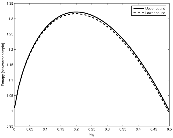
Figure 3: Bounds on information rate. Lower and upper bounds as a function of $p_{W}$ for the binary wall with $p_{X}=1/2$ and $L=9$.

III-B Memory constrained coding

From source-coding theory, the entropy rate $H(V)$ can be attained with an encoder-decoder pair with unbounded memory and delay. In the finite memory case, often the encoder has to code $V_{t}$ based on the observation of $V_{t-1},\dots,V_{t-M}$, and the decoder proceeds accordingly. This situation is similar to one encountered in video compression, where a frame at time $t$ is coded based on $M$ previously coded frames [9]. In this case, the average code-length is bounded below by the conditional entropy $H(V_{t}|V_{t-1},\ldots,V_{t-M})=H(V_{M}|V_{M-1},\ldots,V_{0})$. The bound (7) in Theorem 1 describes the behavior of the conditional entropy $H(V_{M}|V^{M-1})$. Intuitively, by looking at the stored samples from $t-M$ up to $t$, the encoder can separately code $W_{t}$ and take advantage of recurrences present from $t-M$ to $t-1$. In effect, finite memory prevents the encoder to exploit long term recurrences that are not visible in the memory. Similar observations are verified in practice for instance in [13, 12, 14].

Figure 4 illustrates how memory influences coding when $X$ is uniform over an alphabet of size $|{\cal X}|=256$. The curves are computed using the upper bound in (7). Because the alphabet size is large, the bound is tight. In the most recurrent case with $p_{W}=0.5$, the conditional entropy approaches the entropy rate at a slower rate when $M\rightarrow\infty$ [see (7-8)]. Furthermore, as $M$ approaches infinity, there is a significant reduction in the conditional entropy. For instance, an encoder that uses 1 frame in the past with optimal coding would need about twice as many bits as one that uses 4 frames. By contrast, when $p_{W}=0.1$, because longer term recurrences are rare, moderate values of $M$ are already enough to attain the limiting rate. As a result there is little to gain by increasing $M$.

The observations drawn from Figure 4 are also verified in practice for instance in [12, 24, 13]. Finally, we point out that the issue of exploiting long term recurrences dates back to Ziv-Lempel [25] in lossless compression. Extension of the Lempel-Ziv algorithm to the lossy case is discussed in [26], and lossless compression of two-dimensional array in [27]. More recently, an universal scheme to optimally scan and predict data in a multidimensional field with applications to video is presented in [28].

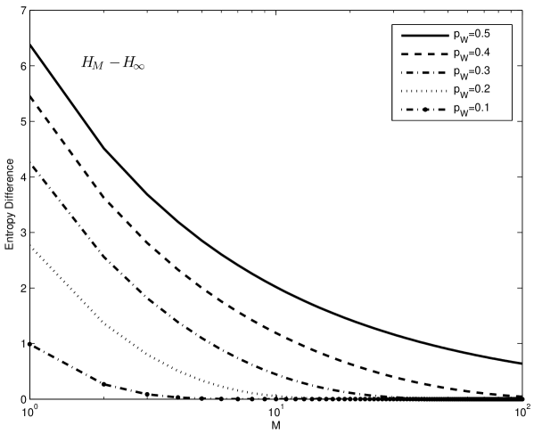
Figure 4: Memory constrained coding. Difference $H(V)-H(V_{M}|V^{M})$ as a function of $M$. When $p_{W}=0.5$, the bit rate can be lowered significantly at the cost of a large memory. A moderate bit rate reduction is obtained with small values of $M$ when $p_{W}=0.1$. The curves are computed using Theorem 1 for $X$ uniform over an alphabet of size 256.

III-C Lossy information rates

In this section we assume again that the process $X$ is i.i.d. and that $X_{n}$ takes values over a finite alphabet ${\cal X}$. Information rates for the lossy case take the form of a rate-distortion function. Consider a $t$-tuple $(V_{1},\ldots,V_{t})$ where each $V_{j}$ is a random vector taking values in ${\cal X}^{L}$. A reproduction $t$-tuple is denoted by $(\hat{V}_{1},\ldots,\hat{V}_{t})$, and its entries take values on a reproduction alphabet $\hat{\cal X}$. A distortion measure is defined as follows:

$$d(V^{t},\hat{V}^{t})=\frac{1}{tL}\sum_{i=1}^{t}d_{s}(V_{i},\hat{V}_{i}),$$

where $d_{s}:{\cal X}\times{\cal\hat{X}}\rightarrow\mathbb{R}^{+}$ is a distortion measure for an $L$-dimensional vector. For example, for the MSE metric we have $d(V_{i},\hat{V}_{i})=\|V_{i}-\hat{V}_{i}\|^{2}$.

The rate-distortion function for each $t$, and for given distortion measure, is written as

$$R_{V^{t}}(D)=\inf_{\mathbb{E}d(V^{t},\hat{V}^{t})\leq D}\frac{I(V^{t};\hat{V}^{t})}{t},$$ (19)

where the infimum of the normalized mutual information $\frac{I(V^{t};\hat{V}^{t})}{t}$ is taken over all conditional pdf’s ${\text{Pr}}\left\{\hat{V}^{t}|V^{t}\right\}$ such that $\mathbb{E}d(V^{t},\hat{V}^{t})\leq D$.

The rate-distortion function for the process $V=(V_{1},V_{2},\ldots)$ is given by [20]

$$R_{V}(D)=\lim_{t\rightarrow\infty}R_{V^{t}}(D).$$ (20)

Because the process $V$ is stationary, it can be shown that the above limit always exists (see [20, p. 270], or [29]).

By coding the side information $W^{t}$ separately, an upper bound for $R_{V}(D)$ similar to Theorem 1 can be developed. The upper bound is based on the notion of conditional rate-distortion [30, 20]. This notion is developed in the lemma below.

Lemma 2

(Gray [30]) Let $V$ be a random vector taking values in ${\cal X}$ and let $W$ be another random variable. Define the conditional rate-distortion:

$$R_{V|W}(D)=\inf_{\mathbb{E}d(V,\hat{V})\leq D}I(V;\hat{V}|W),$$ (21)

where the infimum is taken over all conditional distributions of $\hat{V}$ given $V$ and $W$. The conditional rate-distortion obeys

$$R_{V|W}(D)\leq R_{V}(D)\leq R_{V|W}(D)+I(V;W).\\$$ (22)

The conditional rate-distortion of $V^{t}$ conditioned on $W^{t}$ is defined as follows:

$$R_{V^{t}|W^{t}}(D)=\inf_{\mathbb{E}d(V^{t},\hat{V}^{t})\leq D}\frac{I(V^{t};\hat{V}^{t}|W^{t})}{t},$$ (23)

where the infimum is taken over all probability distributions of $\hat{V}^{t}$ conditional on $V^{t}$ and $W^{t}$. The conditional rate-distortion can be bounded in terms of the rate-distortion function of the process $X$.

Proposition 1

The conditional rate-distortion function satisfies

$$\limsup_{t\rightarrow\infty}R_{V^{t}|W^{t}}(D)\leq(1-2p_{W})R_{X}(D).$$ (24)

Proof:

Let $\lambda(w^{t})$ denote the number of new sites from the path $w^{t}$. Then, conditional on $w^{t}$, the $V^{t}$ has only $\lambda(w^{t})$ entries that need to be encoded. For each $(w^{t},v^{t})$, let $f_{w^{t}}(v^{t})$ denote the vector with the $\lambda(w^{t})$ entries of $v^{t}$ to be coded. Moreover, let $V$ and $\hat{V}$ be such that $\mathbb{E}d_{s}(V_{i}[j],\hat{V}_{i}[j])\leq D$ for $i=0,\ldots,t$, and $j=0,\ldots,L-1$. We have

$$I(V^{t};\hat{V}^{t}|W^{t}) = \sum_{w^{t}}{\text{Pr}}\left\{W^{t}=w^{t}\right\}I(V^{t};\hat{V}^{t}|W^{t}=w^{t})$$ (25)

$$\geq \sum_{w^{t}}{\text{Pr}}\left\{W^{t}=w^{t}\right\}I(f_{w^{t}}(V^{t});f_{w^{t}}(\hat{V}^{t})|W^{t}=w^{t})$$

$$\geq \sum_{w^{t}}{\text{Pr}}\left\{W^{t}=w^{t}\right\}\lambda(w^{t})R_{X}(D)$$

$$= \mathbb{E}\lambda(W^{t})R_{X}(D),$$

where we have used the inequality $I(X;Y)\geq I(f(X);g(Y))$ for measurable functions $f,g$ [31], and the fact that the process $X$ is i.i.d. and independent of $W^{t}$, and that the individual distortions are less than $D$. The lower bound can be achieved as follows. Let $p_{*}(\hat{X}|X)$ be the test channel that attains $R_{X}(D)$. We let $\hat{X}_{n}$ be the result of passing $X_{n}$ though the channel $p_{*}(\hat{X}_{n}|X_{n})$. For each given $w^{t}$ we construct $\hat{V}^{t}$ from $\hat{X}$ and $w_{t}$. This results in a joint conditional distribution that attains the lower bound (25).

Because the lower bound is attainable, it follows that

$$R_{V^{t}|W^{t}}(D)\leq\frac{\mathbb{E}\lambda(W^{t})}{t}R_{X}(D).$$

Moreover, using Lemma 1 it is straightforward to check that $t^{-1}\mathbb{E}\lambda(W^{t})$ converges to $(1-2p_{W})$, which concludes the proof. ∎

The above proposition enables us to derive an upper bound for the rate-distortion function.

Theorem 2

Consider the i.i.d. process $X$ such that $X_{n}$ takes values over a finite alphabet ${\cal X}$. Let $R_{X}(D)$ denote its rate-distortion function. The rate-distortion function of the process $V$ satisfies

$$R_{V}(D)\leq H(p_{W})+(1-2p_{W})R_{X}(D).$$ (26)

Proof:

Using Lemma 2 we have the following bound based on the conditional rate-distortion function [30]:

$$R_{V^{t}|W^{t}}(D)\ \leq\ R_{V^{t}}(D) \leq R_{V^{t}|W^{t}}(D)+\frac{1}{t}I(V^{t};W^{t})$$

$$\leq R_{V^{t}|W^{t}}(D)+H(p_{W}).$$

Letting $t\rightarrow\infty$ and using Proposition 1 asserts (26). ∎

Remark 5

To describe $V^{t}$ to the decoder with average expected distortion less than $D$ we do as follows. Covey the trajectory $W^{t}$ to the decoder spending on average $\approx tH(p_{W})$ bits. Then describe the “spatial innovations” with an average expected distortion less than $D$ spending $\approx\lambda_{t}R_{\cal X}(D)$ bits where $\lambda_{t}\approx t(1-2p_{W})$ is the number of new sites visited up to time $t$. On average, by using this scheme, one needs $H(p_{W})+(1-2p_{W})R_{\cal X}(D)$ bits which is the upper bound presented in (26).

Remark 6

Because the alphabet is finite, if the reproduction alphabet $\hat{\cal X}$ is a superset of the original alphabet ${\cal X}$ and, in addition, the distortion measure is such that $d(x,\hat{x})=0$ if and only if $x=\hat{x}$, then we have that for each $t$, $R_{V^{t}}(D)$ converges to ${t^{-1}}{H(V^{t})}$ as $D\rightarrow 0$ [20]. Consequently, for large alphabet sizes and large block length, the entropy rate bound of (26) is sharp, and so the above bound on the rate-distortion is also sharp for small distortion values.

Theorem 2 shows that in the low distortion regime, optimal encoding in the information-theoretic sense can be attained by extracting and coding $W^{t}$ losslessly, and using the remaining bits to optimally code the vector samples corresponding to spatial innovations. This statement has implications, for example for high rate video coding, since it indicates that motion should be encoded exactly, with the remaining bits allocated to prediction errors.

IV Information Rates for Dynamic Reality

IV-A Model

The model in the previous section assumes a “static background.” More precisely, the infinite wall process $X$ is drawn at time $0$ and does not change after that. In practice, however, scene background changes with time and a suitable model would have to account for those changes. New information comes fundamentally in two forms: the first consists of information that is “seen” by the camera for the first time, while the second consists of changes to old information (e.g., changes in the background). In this section, we propose a model that accounts for both these sources of new information.

To develop a model for scenes that change over time, we model $X$ as a 2-D random field indexed by $(n,t)\in\mathbb{Z}\times\mathbb{Z}^{+}$. A simple yet rich model for the field is that of a first order Markov model over time, and i.i.d. in space. The random field is defined as follows:

Definition 5

The random field is the field $RF=\{X^{(t)}_{n}:(n,t)\in\mathbb{Z}\times\mathbb{Z}^{+}\},$ such that $(X^{(0)}_{n}:n\in\mathbb{Z})$ is i.i.d. and for each $n\in\mathbb{Z}$, the process $(X^{(t)}_{n}:t\in\mathbb{Z})$ is a first order time-homogeneous Markov process possessing a stationary distribution.

The fact that the random field $(X^{(0)}_{n}:n\in\mathbb{Z})$ is i.i.d. simplifies calculations considerably. One justification for this model is when the field is Gaussian. In such case, independence is attained by a simple linear transformation of the process $(X^{(0)}_{n}:n\in\mathbb{Z})$. It can be shown that such transformation preserves the Markovianity on the time dimension, and the i.i.d. assumption can be justified in this case.

Throughout this section, we assume that the Markov chain of the vector process is already in steady-state. This assumption is common, for example, in calculating rate-distortion functions for Gaussian processes with memory [20].

The dynamic vector process $V$ is defined similarly to the static case, but now taking snapshots or vectors from the random field:

Definition 6

Let $RF=\{X^{(t)}_{n}:(n,t)\in\mathbb{Z}\times\mathbb{Z}^{+}\}$ be a random field, and let $W$ be a random walk. The dynamic vector process is the process $V=(V_{t}:t\in\mathbb{Z}^{+})$ such that for each $t>0$,

$$V_{t}=(X_{W_{t}}^{(t)},X_{W_{t}+1}^{(t)},\ldots,X_{W_{t}+L-1}^{(t)}).$$

The random field and the corresponding vector process are illustrated in Figure 5.

\psfrag{t}{$t$}\psfrag{n}{$n$}\psfrag{ldots}{$\cdots$}\psfrag{vdots}{\hskip 8.5359pt$\vdots$}\psfrag{X10}{ \tiny$X_{n-1}^{(t)}$}\psfrag{X11}{ \tiny$X_{n}^{(t)}$}\psfrag{X12}{ \tiny$X_{n+1}^{(t)}$}\psfrag{X20}{ \tiny$X_{n-1}^{(t+1)}$}\psfrag{X21}{ \tiny$X_{n}^{(t+1)}$}\psfrag{X22}{ \tiny$X_{n+1}^{(t+1)}$}\psfrag{X30}{ \tiny$X_{n-1}^{(t+1)}$}\psfrag{X31}{ \tiny$X_{n}^{(t+2)}$}\psfrag{X32}{ \tiny$X_{n+1}^{(t+2)}$}\includegraphics[width=184.9429pt]{random_field.eps}

\psfrag{t}{$t$}\psfrag{n}{$n$}\psfrag{ldots}{$\cdots$}\psfrag{vdots}{\hskip 8.5359pt$\vdots$}\psfrag{X10}{ \tiny$X_{n-1}^{(t)}$}\psfrag{X11}{ \tiny$X_{n}^{(t)}$}\psfrag{X12}{ \tiny$X_{n+1}^{(t)}$}\psfrag{X20}{ \tiny$X_{n-1}^{(t+1)}$}\psfrag{X21}{ \tiny$X_{n}^{(t+1)}$}\psfrag{X22}{ \tiny$X_{n+1}^{(t+1)}$}\psfrag{X30}{ \tiny$X_{n-1}^{(t+1)}$}\psfrag{X31}{ \tiny$X_{n}^{(t+2)}$}\psfrag{X32}{ \tiny$X_{n+1}^{(t+2)}$}\psfrag{t}{$t$}\psfrag{n}{$n$}\psfrag{ldots}{ }\psfrag{vdots}{\hskip 5.69046pt $\vdots$}\psfrag{X00}{\tiny$X_{0}^{(0)}$}\psfrag{X01}{\tiny$X_{1}^{(0)}$}\psfrag{X02}{\tiny$X_{2}^{(0)}$}\psfrag{X10}{\tiny$X_{1}^{(1)}$}\psfrag{X11}{\tiny$X_{2}^{(1)}$}\psfrag{X12}{\tiny$X_{3}^{(1)}$}\psfrag{X20}{\tiny$X_{0}^{(2)}$}\psfrag{X21}{\tiny$X_{1}^{(2)}$}\psfrag{X22}{\tiny$X_{2}^{(2)}$}\psfrag{X30}{\tiny$X_{0}^{(3)}$}\psfrag{X31}{\tiny$X_{1}^{(3)}$}\psfrag{X32}{\tiny$X_{2}^{(3)}$}\includegraphics[width=184.9429pt]{field_random_mov.eps}

Figure 5: A model for the dynamic reality. (a) First, there is a random field that is Markov in the time dimension $t$, and i.i.d. in the spatial dimension $n$. (b) Motion then occurs within this random field.

We point out here that the proposed random field model is a simplified depiction of real visual scene data. For instance, we acknowledge that the spatial independence assumption in non-Gaussian cases is not met in practice, and that the camera motion is not i.i.d. in practice. We stress however that true rate-distortion bounds are difficult to derive for more elaborated sources, and that even a simplified model with true coding bounds is useful provided its deficiencies are acknowledged.

IV-B Lossless information rates

In the development that follows we assume, for simplicity, that the random field takes values on a finite alphabet ${\cal X}$. The results can equally be developed for a random field taking values over $\mathbb{R}$, under suitable technical conditions.

To derive bounds for $H(V)$ in the dynamic reality case, we compute the following conditional entropy rate:

$$H(V|W):=\lim_{t\rightarrow\infty}H(V_{t}|V^{t-1},W^{t}),$$ (27)

if the limit exists. As we shall see in the examples that follow, the above limit can be computed analytically. The key is to compute $H(V_{t}|V^{t-1},W^{t}=w^{t})$ by splitting the set of all paths into recurrent and nonrecurrent paths, and further splitting the set of recurrent paths according to (2).

Referring to Figure 5(b), let $w^{t}$ be a given path and consider the process $V^{t}$. Note that each $V_{t}$ has $L-1$ entries from the same spatial location as $L-1$ entries from $V_{t-1}$. The remaining entry corresponds to either a nonrecurrent or a recurrent location depending on $w^{t}$. If $w^{t}$ is nonrecurrent, then by the Markov property of the field, we have

$$H(V_{t}|V^{t-1},W^{t}=w^{t})=H(X_{0}^{(t)})+(L-1)H(X_{0}^{(t)}|X_{0}^{(t-1)}).$$

If a path is recurrent at $t$, then there is an $s<t$ such that $w_{s}=w_{t}$ but $w_{t}\neq w_{i},$ for $s<i<t$. Using the Markov property again, it follows that $H(V_{t}|V^{t-1},W^{t}=w^{t})=H(X_{0}^{(t)}|X_{0}^{(s)})+(L-1)H(X_{0}^{(t)}|X_{0}^{(t-1)})$. The above argument is explicitly written as follows:

$$H(V_{t}|V^{t-1},W^{t}) = \sum_{w^{t}\in\overline{{\cal R}^{t}}}H(V_{t}|V^{t-1},W^{t}=w^{t}){\text{Pr}}\left\{W^{t}=w^{t}\right\}$$

$$\ \ \ \ \ \ \ +\sum_{w^{t}\in{\cal R}^{t}}H(V_{t}|V^{t-1},W^{t}=w^{t}){\text{Pr}}\left\{W^{t}=w^{t}\right\}$$

$$= \left(H(X_{0}^{(t)})+(L-1)H(X_{0}^{(t)}|X_{0}^{(t-1)})\right){\text{Pr}}\left\{\overline{{\cal R}}^{t}\right\}$$

$$\ \ \ \ \ \ +\sum_{i=1}^{\lfloor t/2\rfloor}\sum_{w^{t}\in{\cal T}_{t-2i}^{t}}H(V_{t}|V^{t-1},W^{t}=w^{t}){\text{Pr}}\left\{W^{t}=w^{t}\right\}$$

$$= \left(H(X_{0}^{(t)})+(L-1)H(X_{0}^{(t)}|X_{0}^{(t-1)})\right){\text{Pr}}\left\{\overline{{\cal R}}^{t}\right\}$$

$$\ \ \ \ \ \ +\sum_{i=1}^{\lfloor t/2\rfloor}\left[\ (H(X_{0}^{(t)}|X_{0}^{(t-2i)})+(L-1)H(X_{0}^{(t)}|X_{0}^{(t-1)})\right){\text{Pr}}\left\{{\cal T}_{t-2i}^{t}\right\}$$

$$= (L-1)H(X_{0}^{(t)}|X_{0}^{(t-1)})+H(X_{0}^{(t)}){\text{Pr}}\left\{\overline{{\cal R}}^{t}\right\}$$

$$\ \ \ \ \ \ \ +\sum_{i=1}^{\lfloor t/2\rfloor}H(X_{0}^{(2i)}|X_{0}^{(0)}){\text{Pr}}\left\{{\cal T}_{0}^{2i}\right\}.$$ (31)

By letting $t\rightarrow\infty$ using Lemma 1 (i) leads to

$$H(V|W)=H(X_{0}^{(\infty)})(1-2p_{W})+(L-1)H(X^{(1)}_{0}|X^{(0)}_{0})+\sum_{i=1}^{\infty}H(X^{(i)}_{0}|X^{(0)}_{0}){\text{Pr}}\left\{{\cal T}^{i}\right\},$$ (32)

where ${\text{Pr}}\left\{{\cal T}^{i}\right\}$ is the probability of return given in Lemma 1 (ii). The infinite sum in the left-hand side of (32) is well-defined. It is an infinite sum of positive numbers, and it is bounded above by $H(X_{0}^{(\infty)})\sum_{i=1}^{\infty}{\text{Pr}}\left\{{\cal T}^{i}\right\}=H(X^{(\infty)})2p_{W}.$ Note that we replaced $2i$ with $i$ in the infinite sum above in view of the fact that ${\text{Pr}}\left\{{\cal T}^{2i+1}\right\}=0$.

With the conditional entropy rate in (32) we can derive lower and upper bounds on the entropy rate $H(V)$. To derive an upper bound, we bound $\frac{H(V^{t})}{t}$ for each $t$ and let $t\rightarrow\infty$. For the lower bound, similar to Section III, we bound $H(V_{t}|V^{t-1})$ below. Because the alphabet ${\cal X}$ is finite and the process is stationary, the limits of $\frac{H(V^{t})}{t}$ and $H(V_{t}|V^{t-1})$ as $t\rightarrow\infty$ coincide.

The upper bound is obtained from the inequality $H(V^{t})\leq tH(p_{W})+H(V^{t}|W^{t})$. Note that $H(V^{t}|W^{t})=\sum_{i=1}^{t}H(V_{i}|V^{i-1},W^{t})$, so that if $H(V_{i}|V^{i-1},W^{t})$ converges to a limit as $t\rightarrow\infty$, we have necessarily that $t^{-1}H(V^{t}|W^{t})$ converges to the same limit (see e.g., [23, p. 64]). So,

$$\lim_{t\rightarrow\infty}\frac{H(V^{t})}{t} \leq H(p_{W})+\lim_{t\rightarrow\infty}\frac{H(V^{t}|W^{t})}{t}$$

$$= H(p_{W})+\underbrace{\lim_{t\rightarrow\infty}H(V_{t}|V^{t-1},W^{t})}_{H(V|W)}.$$

To derive a lower bound, note that the development leading to (13-14) for the static case also holds for the dynamic case. So, we have

$$H(V^{t}|V^{t-1})\geq H(p_{W})+H(V_{t}|V^{t-1},W^{t})-H(W_{t}|V^{t},W^{t-1}).$$ (33)

Thus, a lower bound is obtained by finding an upper bound for $H(W_{t}|W^{t-1},V^{t})$. Because the process $X$ changes at each time step, we cannot use the event $A_{L}$ to obtain an upper bound for $H(W_{t}|W^{t-1},V^{t})$ as in the static case. A useful upper bound for $H(W_{t}|W^{t-1},V^{t})$ is obtained by using Fano’s inequality. Let $P_{e}$ denote the probability of error in estimating $W_{t}$ based on observing $Y_{t}:=(V_{t},V_{t-1},W_{t-1})$, i.e.,

$$P_{e}={\text{Pr}}\left\{\hat{W}(Y_{t})\neq W_{t}\right\},$$

where $\hat{W}(\cdot)$ is a given estimator assumed to be the same for all $t$. Since $W_{t-1}$ is observed, estimating $W_{t}$ amounts to estimating the increment $N_{t}=W_{t}-W_{t-1}$. Because $V$ is stationary and $N_{t}$ is i.i.d., it follows that $P_{e}$ does not depend on $t$. From Fano’s inequality, we have that

$$H(W_{t}|V^{t},W^{t-1}) \leq H(N_{t}|Y_{t})$$ (34)

$$\leq H(P_{e})+P_{e}\log_{2}(1)$$

$$= H(P_{e}).$$

Consequently, a lower bound is obtained by combining (33) with (34) above. By letting $t\rightarrow\infty$ we arrive at the following:

Theorem 3

Consider the vector process $V$ consisting of $L$-tuples generated by a Bernoulli random walk with transition probability $p_{W}$ with $p_{W}\leq 1/2$, and the random field $RF=\{X^{(t)}_{n}:(n,t)\in\mathbb{Z}\times\mathbb{Z}^{+},|{\cal X}|<\infty\}$ that is i.i.d. in the $n$ dimension and first-order Markov in the $t$ dimension. The entropy rate of the process $V$ obeys

$$H(p_{W})+H(V|W)-H(P_{e})\leq H(V)\leq H(p_{W})+H(V|W),$$ (35)

where $H(V|W)$ is as in (32), and $P_{e}$ is the probability of error in estimating $W_{1}$ based on the observation of $Y_{1}=(V_{1},V_{0},W_{0})$ with any estimator $\hat{W}(Y_{1})$.

The lower and upper bounds become sharp when $P_{e}\rightarrow 0$. This occurs with large block sizes and for small changes in the background. The examples that follow illustrate the sharpness of the above bounds. In the first example, we consider a binary process $X$, and on the second a Gaussian process with AR(1) temporal innovations.

\psfrag{BSC}{\small BSC}\psfrag{ldots}{$\ldots$}\psfrag{vdots}{\hskip 11.09654pt$\vdots$}\psfrag{Xt0}{ \footnotesize$X_{n-1}^{(t)}$}\psfrag{Xt1}{ \footnotesize$X_{n}^{(t)}$}\psfrag{Xt2}{ \footnotesize$X_{n+1}^{(t)}$}\psfrag{Yt0}{ \footnotesize$X_{n-1}^{(t+1)}$}\psfrag{Yt1}{ \footnotesize$X_{n}^{(t+1)}$}\psfrag{Yt2}{ \footnotesize$X_{n+1}^{(t+1)}$}\includegraphics[width=199.16928pt]{wall_innov_nomov.eps}

Figure 6: The binary random field. Innovations are in the form of bit flips caused by binary symmetric channels between consecutive time instants.

Example 2

BSC innovations
Suppose that at $t=0$, the process is a strip of bits that are i.i.d. Bernoulli with initial distribution $p_{X}$. Suppose that from $t$ to $t+1$ there is a nonzero probability $p_{I}$ that the bit $X_{n}^{(t)}$ is flipped. This amounts to a binary symmetric channel (BSC) between $X_{n}^{(t)}$ and $X_{n}^{(t+1)}$, as illustrated in Figure 6. The $t$ BSCs in series between $X_{n}^{(0)}$ and $X_{n}^{(t)}$ are equivalent to a single BSC with transition probability (see [23, p. 221], problem 8)

$$p_{I,t}=0.5\left(1-(1-2p_{I})^{t}\right).$$ (36)

Note that for $p_{I}>0$, we have that $\lim_{t\rightarrow\infty}p_{I,t}=0.5$. So, for each $n$, the distribution of $X_{n}^{(t)}$ converges to the stationary distribution $Bern(0.5)$. Substituting in (32) gives for $p_{I}>0$:

$$H(V|W)=H(\frac{1}{2})(1-2p_{W})+(L-1)H(p_{I})+\sum_{i=1}^{\infty}H(p_{I,2i}){\text{Pr}}\left\{{{\cal T}}_{0}^{2i}\right\}.$$ (37)

Notice that when $p_{I}=0$ we recover the static case. By using the above in (35) we obtain the corresponding bounds. Figure 7 (a) illustrates the lower and upper bounds for $L=8$ and $p_{X}=0.5$. We compute the bounds using (32) and (35), where we truncate the infinite sum in (32) at a very large $t$. The probability $P_{e}$ is computed through Monte Carlo simulation using a simple Hamming distance detector. The bounds are surprisingly robust in this case, and provide good approximation of the true entropy rate. Notice that when $p_{I}$ increases, the entropy rate of the recurrent case ($p_{W}=0.5$) crosses that of the panning case ($p_{W}=0.05$). This is because in the recurrent case a greater amount of bits is spent coding the innovations.

Figure 7 (b) shows the contour plots of the upper bound for various pairs $(p_{I},p_{W})$. The plot shows how the two innovations are combined to generate a given entropy value. Notice that when $p_{W}$ approaches $\frac{1}{2}$, the entropy of the trajectory becomes significant and it compensates for the lesser amount of spatial innovation.

To measure the effect of memory in the dynamic case, we evaluate the upper bound on the conditional entropy rate (as in (11)), and the upper bound on the true entropy rate given by (3). Figure 8 illustrates the difference between the conditional entropy upper bound and the true entropy upper bound. The curves are similar to the ones obtained in the static case with spatial innovation (Figure 4), and confirm the very intuitive fact that memory is less useful when the scene around changes rapidly.

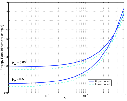
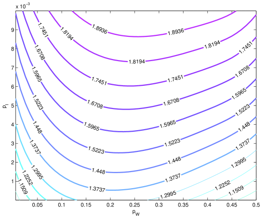
Figure 7: The binary symmetric innovations. (a) The curves show the lower and upper bounds on the entropy rate. Notice that the bounds are sharp for various values of $p_{I}$. (b) Contour plots of the upper bound for various $p_{I}$ and $p_{W}$. The lines indicate points of similar entropy but with different amounts of spatial and temporal innovation.

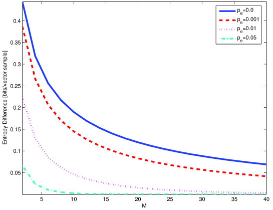
Figure 8: Memory and innovations. Shown is the difference between the conditional entropy and the true entropy for the binary innovations with $p_{X}=0.5$, $p_{W}=0.5$, and $L=8$. The curves show the intuitive fact that when the background changes too rapidly, there is little to be gained in bitrate by utilizing more memory.

Example 3

AR(1) Innovations.

Although the development leading to Theorem 3 was made for finite alphabets, the same calculation can be done for a random field taking values on $\mathbb{R}$, provided it has absolutely continuous joint densities. In this case, the entropies involved become differential entropies. For example, for each $n\in\mathbb{Z}$ and $0<\rho<1$, let

$$X_{n}^{(t)}=\rho X_{n}^{(t-1)}+\epsilon_{t}$$

for $t\in\mathbb{Z}^{+}$, where $\epsilon_{t}\sim N(0,1-\rho^{2})$ i.i.d. and independent of $X$. Such a random field model is used for instance in [32] for bit allocation over multiple frames. Let $\phi(\sigma^{2})$ denote the differential entropy of a Gaussian density with variance $\sigma^{2}$:

$$\phi(\sigma^{2}):=\frac{1}{2}\log_{2}(2\pi e\sigma^{2}).$$

It is then easy to check that $h(X_{1}^{(\infty)})=\phi(1)$, and $h(X^{(i)}_{1}|X^{(0)}_{1})=\phi(1-\rho^{2i})$, so that we obtain a lower and an upper bound on the differential entropy rate using Theorem 3. The conditional differential entropy rate $h(V|W)$ is

$$h(V|W)=\phi(1)(1-2p_{W})+(L-1)\phi(1-\rho^{2})+\sum_{i=1}^{\infty}\phi\left(1-\rho^{4i}\right){\text{Pr}}\left\{{{\cal T}}_{0}^{2i}\right\}.$$ (38)

The infinite sum on the right-hand side is well defined. Because $1-\rho^{2k}$ converges to $1$ as $k\rightarrow\infty$ we see that for any value of $\rho$ in $(-1,1)$, the tail of the infinite sum is a sum of positive numbers. Using (4) and Lemma 1 (i), we see that $\sum_{i=1}^{\infty}{\text{Pr}}\left\{{{\cal T}}_{0}^{2i}\right\}=2p_{W}$. Because $\phi(\cdot)$ is concave, we can use Jensen’s inequality as follows:

$$\sum_{k=1}^{\infty}\phi(1-\rho^{4k}){\text{Pr}}\left\{{\cal T}_{0}^{2k}\right\} = 2p_{W}\sum_{k=1}^{\infty}\phi(1-\rho^{4k})\frac{{\text{Pr}}\left\{{\cal T}_{0}^{2k}\right\}}{2p_{W}}$$

$$\leq 2p_{W}\phi\left(\sum_{k=1}^{\infty}(1-\rho^{4k})\frac{{\text{Pr}}\left\{{\cal T}_{0}^{2k}\right\}}{2p_{W}}\right).$$

Using Lemma 1 (ii) and the generating function for the Catalan numbers [33], one can further check that

$$\sum_{k=1}^{\infty}(1-\rho^{4k}){{\text{Pr}}\left\{{\cal T}_{0}^{2k}\right\}}=((1-4(1-p_{W})p_{W}\rho^{4}))^{1/2}-(1-2p_{W}),$$

so that the last term is controlled by

$$\sum_{k=1}^{\infty}\phi(1-\rho^{4k}){\text{Pr}}\left\{{\cal T}_{0}^{2k}\right\}\leq 2p_{W}\phi\left(\frac{(1-4(1-p_{W})p_{W}\rho^{4})^{1/2}-(1-2p_{W})}{2p_{W}}\right).\\$$ (39)

The above upper bound turns out to be a very good approximation of the infinite sum in (38) when $p_{W}$ is close to $0$, and when $\rho$ is away from $1$.

Notice that for $L$ large and $\rho$ close to 1, $P_{e}$ and $H(P_{e})$ are small so that the bounds in Theorem 3 are sharp. Figure 9 displays the bounds on the differential entropy as a function of $\rho$. The bounds are computed following Theorem 3 and (38). Here $P_{e}$ is inferred via Monte Carlo simulation with $10^{7}$ trials, and a minimum MSE detector for $W_{t}$. The inferred $P_{e}$ is so low that the lower and upper bounds practically coincide. Analytical computation of $P_{e}$ is a detection problem beyond the scope of this papers.

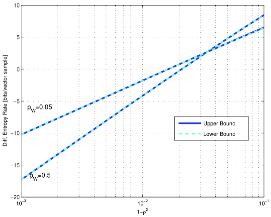
Figure 9: Differential entropy bounds for the Gaussian AR(1) case as function of the innovation parameter $\rho$. In this example $P_{e}$ is small enough that the lower and upper bounds practically coincide. Note that the slope of the differential entropy curve is influenced by the value of $p_{W}$.

IV-C Lossy information rates for the AR(1) random field

Consider the AR(1) innovations of the previous example. Under the MSE distortion measure it is possible to derive an upper bound to the lossy information rate. The key is to compute $R_{V^{t}|W^{t}}(D)$ defined as in (23) and use the upper bound [30]:

$$R_{V^{t}}(D)\leq H(p_{W})+R_{V^{t}|W^{t}}(D),$$ (40)

for each $t>0$. The conditional rate-distortion satisfies the Shannon lower bound (SLB) [20]:

$$R_{V^{t}|W^{t}}(D)\geq\frac{h(V^{t}|W^{t})}{t}-L\phi(D).$$ (41)

The key observation is that for a given fixed trajectory $w^{t}$, the rate-distortion function of $V^{t}$ is that of a Gaussian vector consisting of the samples of the random field covered by $W^{t}$. For a Gaussian vector, the SLB is tight when the per sample distortion is less than the minimum eigenvalue of the covariance matrix (see [20, p. 111]). The next proposition gives a condition under which (41) is tight, and thus when combined with (40) provides an upper bound on the rate-distortion function.

Proposition 2

Consider the vector process $V$ resulting from the Gaussian AR(1) random field with correlation coefficient $0<\rho<1$, and a Bernoulli random walk with probability $p_{W}\leq 1/2$. The Shannon lower bound for the conditional rate-distortion function is tight whenever the distortion satisfies

$$0<D<\frac{1-\rho}{1+\rho}.$$ (42)

To assert the claim we rely on the following lemmas:

Lemma 3

Let $X_{1},X_{2},\ldots,X_{m}$ be a sequence of Gaussian vectors in $\mathbb{R}^{d}$ such that $X_{j}\sim N(0,C_{j})$, and where each $C_{j}$ has spectrum $\lambda(C_{j})$. Let $W$ be a random variable independent of $X_{1},\ldots,X_{m}$ such that ${\text{Pr}}\left\{W=j\right\}=\mu_{j}$ for $j=1,\ldots,m$. Consider the mixture

$$X=\sum_{j=1}^{m}\mathbb{I}_{\{W=j\}}X_{j}.$$ (43)

Denote by $R_{X|W}(D)$ the conditional rate-distortion with per-sample MSE distortion $D$. Then, if

$$D\leq\min\bigcup_{j=1}^{m}\lambda(C_{j}),$$ (44)

the conditional rate distortion function is

$$R_{X|W}(D)=\sum_{j=1}^{m}\mu_{j}R_{X_{j}}(D).$$ (45)

Proof:

Let $p(X,\hat{X}|W)$ be such that ${d}^{-1}\ \mathbb{E}\|X-\hat{X}\|^{2}\leq D$. Then,

$$I(X;\hat{X}|W) = \sum_{j=1}^{m}\mu_{j}I(X;\hat{X}|W=j)$$ (46)

$$\geq \sum_{j=1}^{m}\mu_{j}R_{X_{j}}(D_{j})$$ (47)

with

$${d}^{-1}\mathbb{E}\|X-\hat{X}\|^{2}=\sum_{j=1}^{m}\mu_{j}D_{j}\leq D,$$ (48)

and $D_{j}:={d}^{-1}\ \mathbb{E}(\|X-\hat{X}\|^{2}|W=j)$. The above is minimized when

$$R_{X_{j}}^{\prime}(D_{j})=\theta,$$ (49)

where $\theta$ is some constant. Suppose $D\leq\min\bigcup_{j=1}^{m}\lambda(C_{j})$ and $D_{j}=D$. We have

$$R_{X_{j}}(D_{j})=\frac{1}{d}\sum_{p=1}^{d}\frac{1}{2}\log_{2}(\frac{\lambda_{j,p}}{D}),$$ (50)

where $\lambda_{j,p}$ are the eigenvalues of $C_{j}$ and moreover $R^{\prime}_{X_{j}}(D_{j})=-\frac{1}{2D_{j}}=-\frac{1}{2D}$ so that conditions for a minimum are satisfied. The lower bound can be attained by setting

$$p(X,\hat{X}|W=j)=p_{j}^{*}(X,\hat{X}),$$

where $p_{j}^{*}(X_{j},\hat{X}_{j})$ attains $R_{X_{j}}(D_{j})$. ∎

Lemma 4

([34, p. 189]) Let A be a $n\times n$ Hemitian matrix, and let $1\leq m\leq n$. Let ${\text{A}}_{m}$ denote a principal submatrix of A, obtained by deleting $n-m$ rows and the corresponding columns of A. Then, for each integer $k$ such that $1\leq k\leq m$, we have

$$\lambda_{k}({\text{A}})\leq\lambda_{k}({\text{A}}_{k}),$$ (51)

where $\lambda_{k}({\text{A}})$ denotes the $k$-th largest eigenvalue of matrix A.

Proof of Proposition 2: The SLB for each $t>0$ is given by

$$R_{V^{t}|W^{t}}(D)\geq\frac{h(V^{t}|W^{t})}{t}-L\phi(D).$$ (52)

Because

$$I(V^{t};\hat{V}^{t}|W^{t})=\sum_{W^{t}=w^{t}}{\text{Pr}}\left\{W^{t}=w^{t}\right\}I(V^{t};\hat{V}^{t}|W^{t}=w^{t}),$$

in view of Lemma 3, it suffices to show that for each $t>0$, and for $0\leq D\leq\frac{1-\rho}{1+\rho}$, the bound

$$\frac{I(V^{t};\hat{V}^{t}|w^{t})}{t}\geq\frac{h(V^{t}|w^{t})}{t}-L\phi(D),\text{ for }\mathbb{E}(d(V^{t},\hat{V}^{t})|w^{t})\leq D$$

is achievable. Given $W^{t}=w^{t}$, the above bound is attainable if $D$ is smaller than the minimum eigenvalue of the covariance matrix of the random field samples covered by $w^{t}$. Denote this covariance by ${\text{C}}_{w^{t}}:=\text{Cov}(V^{t}|w^{t})$. Because the random field is independent in the spatial dimension $n$, the spectrum of the covariance matrix is the disjoint union of the spectra of the covariance matrices corresponding to the random field samples of $V^{t}$ at similar location $n$. Each ${\text{C}}_{w^{t}}$ is a submatrix of the $t\times t$ Toeplitz matrix ${\text{T}}_{t}(\rho)$ with entries $[{\text{T}}_{t}(\rho)]_{ij}=\rho^{|i-j|}$. Since $\lambda_{min}({\text{T}}_{t}(\rho))$ decreases to $(1-\rho)/(1+\rho)$ as $t\rightarrow\infty$ [35], by applying the Lemma above we conclude that

$$\lambda_{min}({\text{C}}_{w^{t}})\geq\lambda_{min}({\text{T}}_{t}(\rho))\geq\frac{1-\rho}{1+\rho}.$$ (53)

Therefore, the bound (52) is achievable for each $t$ and since the limit of $R_{V^{t}|W^{t}}(D)$ exists it follows that the bound is achievable for $t\rightarrow\infty$.

Example 4

We simulate the AR(1) dynamic reality model. To compress the process $V^{t}$, we estimate the trajectory and send it as side information. With the trajectory at hand, we encode the samples with DPCM, encoding the residual with entropy constrained scalar quantization (ECSQ). We build two encoders. In the first one, prediction is done utilizing only the previously encoded vector sample; in the second, all encoded samples up to time $t$ are available to the encoder (and decoder). Figure 10 illustrates the SNR as a function of rate when the block-length $L=8$. In Figure 10 (a) and (b) we have $\rho=0.99$ and the upper bound is valid for SNR greater than 23 dB. In Figure 10 (a), we have $p_{W}=0.5$. Because the scene changes slowly and is highly recurrent, the infinite memory encoder ($M=\infty$) is about 3.5 dB better than when $M=1$. The same behavior is not observed when the scene is not recurrent (panning case, $p_{W}=0.1$, Figure 10 (b) ), and when the background changes too rapidly ($\rho=0.9$, Figure 10 (c)).

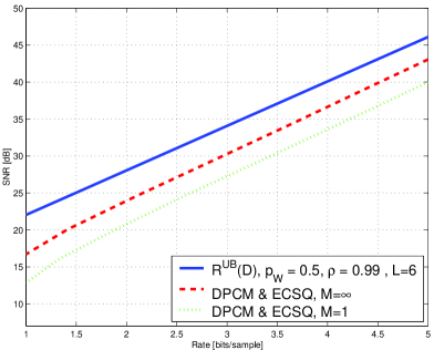
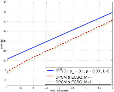
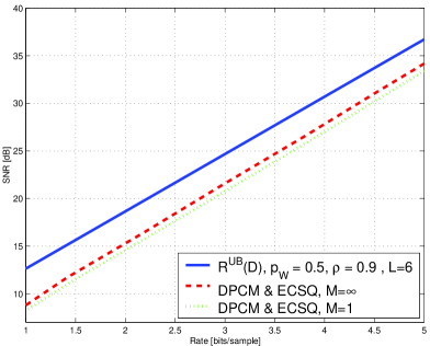
Figure 10: Performance of DPCM with motion for various $\rho$ and $p_{W}$. For $\rho=0.99$ and $\rho=0.9$ the upper bound is valid for SNR greater than 23 dB and 12.8 dB, respectively. (a) Memory provide considerable gains, $p_{W}=0.5,\rho=0.99$. (b) Modest gains when $p_{W}=0.1$. (c) Modest gains when $\rho=0.9$, as background changes too rapidly.

V Conclusion

We have proposed a stochastic model for the plenoptic function that enables the precise computation of information rates. For the static case, we provided lossless and lossy information rate bounds that are tight in a number of interesting cases. In some scenarios, the theoretical results support the ubiquitous hybrid coding paradigm of extracting motion and coding a motion compensated sequence.

We extended the model to account for changes in the background scene, and computed bounds for the lossless and lossy information rates for the particular case of AR(1) innovations. The bounds for this “dynamic reality” are tight in some scenarios, namely when the background scene changes slowly with time (i.e., $\rho$ close to 1).

The model explains precisely how long-term motion prediction helps coding in both static and dynamic cases. In the dynamic model, this is related to the two parameters $(p_{W},\rho)$ that symbolizes the rate of recurrence in motion and the rate of changes in the scene. As $(p_{W},\rho)\rightarrow(0.5,1)$, long term memory predictions result in significant improvements (in excess of 3.5 dB). By contrast, if either $\rho$ is away from 1, or if $p_{W}$ is away from $0.5$, long term memory brings little improvement.

Although we developed the results for the Bernoulli random walk, the model can be generalized to other random walks on $\mathbb{Z}$ and $\mathbb{Z}^{2}$. Our current work includes such generalizations. It also includes estimating $\rho$ and $p_{W}$ for real video signals and fitting the model to such signals.

References

- [1] A. L. da Cunha, M. N. Do, and M. Vetterli, “A stochastic model for video and its information rates,” in Prof. of IEEE Data Compression Conference (DCC), March 2007, pp. 3–12.
- [2] E. H. Adelson and J. R. Bergen, “The plenoptic function and the elements of early vision,” in Computational Models of Visual Processing, M. Landy and J. A. Movshon, Eds. Cambridge, UK: MIT Press, 1991, pp. 3–20.
- [3] D. Forsyth and J. Ponce, Computer Vision: A Modern Approach. Englewood Cliffs, NY: Prentice Hall, 2002.
- [4] C. Zhang and T. Chen, “A survey on image-based rendering representation, sampling and compression,” EURASIP Signal Processing: Image Communication, vol. 19, pp. 1–28, Jan. 2004.
- [5] M. Levoy and P. Hanrahan, “Light field rendering,” in Proceedings of SIGGRAPH, 1996, pp. 31–42.
- [6] S. J. Gortler, R. Grzeszczuk, R. Szeliski, and M. Cohen, “The lumigraph,” in Proceedings of SIGGRAPH, 1996, pp. 43–54.
- [7] L.-W. He and H.-Y. Shum, “Rendering with concentric mosaics,” in Proceedings of SIGGRAPH, 1999, pp. 299–306.
- [8] C. Zhang and T. Chen, “Spectral analysis for sampling image-based rendering data,” IEEE Trans. on CSVT Special Issue on Image-Based Modeling, Rendering and Animation, vol. 13, pp. 1038–1050, Nov. 2003.
- [9] A. Telkap, Digital Video Processing. Upper Saddle River, NJ: Prentice-Hall, 1995.
- [10] Y. Wang, J. Ostermann, and Y.-Q. Zhang, Video Processing and Communications. Englewood Cliffs, NJ: Prentice-Hall, 2002.
- [11] J. W. Woods, Multidimensional Signal, Image, and Video Processing and Coding, Academic Press. Academic Press, 2006.
- [12] H. Li and R. Forchheimer, “Extended signal-theoretic techniques for very low bit-rate video coding,” in Video Coding: The Second Generation Approach. Norwell, MA: Kluwer, 1996, pp. 383–428.
- [13] T. Wiegand, X. Zhang, and B. Girod, “Long-term memory motion-compensated prediction,” IEEE Trans. CSVT, vol. 9, no. 1, pp. 70–84, February 1999.
- [14] C. Herley, “ARGOS: Automatically extracting repeating objects from multimedia streams,” IEEE Trans. on Multimedia, vol. 8, no. 1, pp. 115–129, Feb 2006.
- [15] N. Vasconcelos and A. Lippman, “Statistical models of video structure for content analysis and characterization,” IEEE Trans. in Image Proc., vol. 9, no. 1, pp. 3–19, Jan. 2000.
- [16] B. Girod, “The efficiency of motion-compensating prediction for hybrid coding of video sequences,” IEEE Journal of Selected Areas in Communications, vol. SAC-5, no. 7, pp. 1140–1154, August 1987.
- [17] P. Ramanathan and B. Girod, “Rate-distortion analysis for light field coding and streaming,” EURASIP Signal Processing: Image Communication, vol. 21, no. 6, pp. 462–475, July 2006.
- [18] N. Gehrig and P. L. Dragotti, “Geometry-driven distributed compression of the plenoptic function: Performance bounds and constructive algorithms,” IEEE Trans. Image Proc., vol. 18, no. 3, pp. 457–470, March 2009.
- [19] A. Smolic and P. Kauff, “Interactive 3-D video representation and coding technologies,” Proc. of the IEEE, vol. 93, no. 1, pp. 98–110, January 2005.
- [20] T. Berger, Rate-Distortion Theory: A Mathematical Basis for Data Compression. Englewood Cliffs, NJ: Prentice-Hall, 1972.
- [21] J. Rudnick and G. Gaspari, Elements of the Random Walk. Cambridge, UK: Cambridge University Press, 2004.
- [22] W. Feller, An Introduction to Probability Theory and Its Applications. New York, NY: John Wiley and Sons, 1957.
- [23] T. M. Cover and J. A. Thomas, Elements of Information Theory. New York, NY: John Wiley & Sons, 1991.
- [24] N. Vascocelos and A. Lippman, “Library-based image coding,” in Proc. IEEE Int. Conf. Acoust., Speech, and Signal Proc., vol. 5, Adelaide, Australia, April 1994, pp. 489–492.
- [25] J. Ziv and A. Lempel, “Compression of individual sequences via variable-rate coding,” IEEE Transactions on Information Theory, vol. 24, no. 5, pp. 530–536, Sept. 1978.
- [26] Y. Steinberg and M. Gutman, “An algorithm for source coding subject to a fidelity criterion, based on string matching,” IEEE Trans. Inf. Theory, vol. 39, no. 3, pp. 877–886, May 1993.
- [27] A. Lempel and J. Ziv, “Compression of two-dimensional data,” IEEE Trans. Inf. Theory, vol. 32, no. 1, pp. 2–8, 1986.
- [28] A. Cohen, N. Merhav, and T. Weissman, “Scanning and sequential decision making for multidimensional data - part I: The noiseless case,” IEEE Trans. Inf. Theory, vol. 53, no. 9, pp. 3001–3020, Sept. 2007.
- [29] M. S. Pinsker, Information and Information Stability of Random Variables. San Francisco, CA: Holden Day, 1984.
- [30] R. M. Gray, “A new class of lower bounds to information rates of stationary sources via conditional rate-distortion functions,” IEEE Trans. on Info. Theory, vol. IT-19, no. 4, pp. 480–489, July 1973.
- [31] R. M. Gray, Entropy and Information Theory. New York: Springer-Verlag, 1990.
- [32] Y. Sermadevi, J. Chen, S. Hemami, and T. Berger, “When is bit allocation for predictive video coding easy?” in Data Compression Conference (DCC), Snowbird, UT, 2005, pp. 289–298.
- [33] R. L. Graham, D. E. Knuth, and O. Patashnik, Concrete Mathematics: A Foundation for Computer Science. Boston, MA: Addison-Wesley Longman Publishing Co., Inc., 1989.
- [34] R. A. Horn and C. R. Johnson, Matrix Analysis. Cambridge, UK: Cambridge Univ. Press, 1999.
- [35] R. M. Gray, “On the asymptotic eigen-value distribution of Toeplitz matrices,” IEEE Trans. Inf. Theory, vol. 18, no. 6, pp. 725–730, 1972.