Global effects of local sound-speed perturbations in the Sun: A theoretical study

Abstract

We study the effect of localized sound-speed perturbations on global mode frequencies by applying techniques of global helioseismology on numerical simulations of the solar acoustic wave field. Extending the method of realization noise subtraction (e.g. Hanasoge07a) to global modes and exploiting the luxury of full spherical coverage, we are able to achieve very highly resolved frequency differences that are used to study sensitivities and the signatures of the thermal asphericities. We find that (1) global modes are almost twice as sensitive to sound-speed perturbations at the bottom of the convection zone as in comparison to anomalies well in the radiative interior ($r\lesssim 0.55R_{\odot}$), (2) the $m$-degeneracy is lifted ever so slightly, as seen in the $a$ coefficients, and (3) modes that propagate in the vicinity of the perturbations show small amplitude shifts ($\sim 0.5\%$).

1 Introduction

Global helioseismology has proven very successful at inferring large scale properties of the Sun (for a review, see jcd.review; jcd0). Because they are very robust, the extension of methods of global helioseismology to study localized variations in the structure and dynamics of the solar interior has been of some interest (e.g. Swisdak). However, the precise sensitivities of global modes to local perturbations are difficult to estimate through analytical means, especially in cases where the flows or thermal asphericities of interest possess complex spatial dependencies. To address questions relating to sensitivities and with the hope of perhaps discovering hitherto unknown phenomena associated with global modes, we introduce here for the first time a technique to study the effects of arbitrary perturbations on global mode parameters in the linear limit of small wave amplitudes.

Global modes attain resonant frequencies as a consequence of differentially sampling the entire region of propagation, making it somewhat more difficult (in comparison to local helioseismology) to pinpoint local thermal asphericities at depth. Exactly how difficult is one of the questions we have attempted to answer in this article. Jets in the tachocline (e.g. jcd1) are a subject of considerable interest since their existence (or lack thereof) could be very important in understanding the angular momentum balance of the Sun. Studying the sensitivities and signatures of waves to flows at depth may open up possibilities for their detection.

Forward modeling as a means of studying wave interactions in a complex medium like the Sun has become quite favoured (e.g. Hanasoge06; Parchevsky; Hanasoge07a; Cameron). The discovery of interesting phenomena, especially in the realm of local helioseismology (e.g. Hanasoge07b; Birch07), adds motivation to the pursuit of direct calculations. With the application of noise subtraction [Werne, Birch, and Julien (2004), Hanasoge, Duvall, and Couvidat (2007)], we can now study the signatures of a wide range of perturbations in a realistic multiple source picture. Here, we attempt to place bounds on the detectability of thermal asphericities at various depths in the Sun. We introduce and discuss the method of simulation with a description of the types of perturbations introduced in the model in Section 2. The estimation of mode parameters can prove somewhat difficult due to restrictions on the temporal length of the simulation ($<24$ hours; owing to the expensive nature of the computation). The data analysis techniques used to characterize the modes are presented in Section 3. We then discuss the results from the analyses of the simulated data in $\S$4 and summarize this work in $\S$5.

2 Simulations and perturbations

The linearized 3D Euler equations in spherical geometry are solved in the manner described in Hanasoge06. The computational domain is a spherical shell extending from $0.24R_{\odot}$ to $1.002R_{\odot}$, with damping sponges placed adjacent to the upper and lower radial boundaries to allow the absorption of outgoing waves. The background stratification is a convectively stabilized form of model S [Christensen-Dalsgaard et al. (1996), Hanasoge et al. (2006)]; only the highly (convectively) unstable near-surface layers ($r>0.98R_{\odot}$) are altered while the interior is the same as model S. Waves are stochastically excited over a 200 km thick sub-photospheric spherical envelope, through the application of a dipolar source function in the vertical (radial) momentum equation [Hanasoge et al. (2006), Hanasoge and Duvall (2007)]. The forcing function is uniformly distributed in spherical harmonic space $(l,m)$; in frequency, a solar-like power variation is imposed. Any damping of the wave modes away from the boundaries is entirely of numerical origin. The radial velocities associated with the oscillations are extracted 200 km above the photosphere and used as inputs to the peakbagging analyses. Data over the entire 360^∘ extent of the sphere are utilized in the analyses, thus avoiding issues related to mode leakage. We show an example power spectrum in Figure 1 along with the fits.

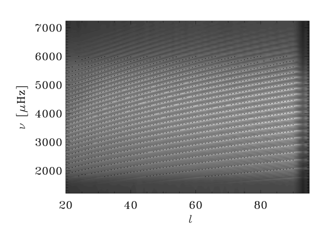
Figure 1.: Example power spectrum from a simulation with $l_{max}=95$ and the corresponding frequency fits (symbols). This is from a 24-hour simulation. The fitting algorithm is described in Section 3. Missing modes indicate that the fit for these did not converge. We do not understand why this occurs in the center of the power spectrum, but these modes can be made to converge by perturbing their initial guesses. Modes with $l<20$ mostly disappear from the computational domain because the lower boundary is placed at $r=0.24R_{\odot}$. We also do not excite the highest $l$ modes because we wish to avoid any issues related to numerical aliasing.

The technique of realization noise subtraction (e.g. Hanasoge07a) is extensively applied in this work. Due to the relatively short time lengths of the simulations (the shortest time series yet that we have worked with is 500 minutes long!), the power spectrum is not highly resolved and it would seem that the resulting uncertainty in the mode parameter fits might constrain our ability to study small perturbations. To beat this limit, we perform two simulations with identical realizations of the forcing function: a ‘quiet’ run with no perturbations, and a ‘perturbed’ run that contains the anomaly of interest. Fits to the mode parameters in these two datasets are then subtracted, thus removing nearly all traces of the realization and retaining only effects arising due to mode-perturbation interactions (see Section 3). As an example, we show in Figure 2 how a localized sound-speed perturbation placed at the bottom of the convection zone scatters waves which then proceed to refocus at the antipode (the principle of farside holography, lindsey). The presence of the sound-speed perturbation is not seen in panel a, whereas it is clearly seen in the noise-subtracted images of panels b and c.

In these calculations, we only consider time-stationary perturbations. The sound-speed perturbations are taken to be solely due to changes in the first adiabatic index, $\Gamma_{1}$; we do not study sound-speed variations arising from changes in the background pressure or density since altering these variables can create hydrostatic instabilities. Lastly, the amplitude of all perturbations are taken to be much smaller than the local sound speed ($\lesssim 5\%$).

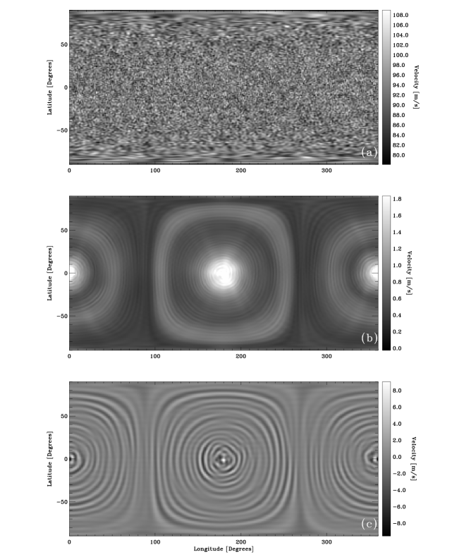
Figure 2.: Noise subtraction at work. Panel a is the time averaged RMS of the radial velocities of the perturbed simulation; the sound-speed perturbation (located along the equator at $r=0.7R_{\odot}$ and 180^∘ longitude) is invisible. In panel b, the time averaged RMS of the difference between the quiet and perturbed simulations and shown in panel c is the instantaneous difference. The scattering of waves and their refocusing at the antipode is clearly seen in b.

3 Peakbagging analysis

Our first round of peakbagging is done on the $m$-averaged power spectrum for the quiet simulation. For each $l$ that we attempt to fit, we search for peaks in the negative second derivative of the power. Unlike the power itself, which has a background, the second derivative has the advantage of having an approximately zero baseline. The search is accomplished by finding the frequency at which the maximum value of the negative second derivative occurs, estimating the mode parameters using a frequency window of width 100 $\mu$Hz centered on this peak frequency, zeroing the negative second derivative in this interval, and iterating. If the range of power in the frequency window is not above a certain threshold, we check the peak frequency found; if it is too close to a frequency found on a previous iteration, that maximum is rejected, the same interval is again zeroed, and iteration continues. Note that such a simple algorithm is feasible only because simulation data contains no leaks. Once we have found as many peaks as possible with this procedure, we assign a value of $n$ to each one based on a model computed using ADIPACK [Christensen-Dalsgaard and Berthomieu (1991), Hanasoge (2007)].

The next step is to perform an actual fit to the power spectrum in the vicinity of each peak we identified. For the line profile we use a Lorentzian of the form

$$P=\frac{A}{\pi}\frac{w}{(\nu-\nu_{0})^{2}+w^{2}}+B,$$ (1)

where $A$ is the total power, $w$ is the half width at half maximum, $\nu_{0}$ is the peak frequency, and $B$ is the background power. The initial guesses for these parameters are obtained in the first step as follows: $B$ is set to the minimum value of the power in the frequency window around the peak, $A$ is set to the integral under the power curve minus $B$ times the width of the window, and $w$ is set to $1/(\pi P_{max})$ where $P_{max}$ is the maximum value of the power in the frequency window. The fitting interval extends halfway to the adjacent peaks, or 100 $\mu$Hz beyond the peak frequency of the modes at the edge. The fitting itself is done using the IDL routine curvefit.

Once we have fit these mode parameters for the $m$-averaged spectrum, we use them as the initial guesses for fitting the individual $m$ spectra. Then for each $l$ and $n$ we can fit a set of $a$-coefficients to the frequencies as functions of $m/l$. Although for the quiet sun we would expect for all the $a$-coefficients to be zero, this calculation is still necessary in order to perform the noise subtraction.

We also use the mode parameters from the $m$-averaged spectrum of the quiet simulation as initial guesses for fitting the (unshifted) $m$-averaged spectrum of the perturbed simulation. Although the perturbations may lift the degeneracy in $m$, we expect the splitting to be very small, so that the peaks in the $m$-averaged spectrum can still be well represented by a Lorentzian. We also use those same initial guesses for fitting the individual $m$ spectra of the perturbed simulation, and recalculate the $a$-coefficients.

An empirical estimate of the error in frequency differences for the sound-speed perturbation at $r=0.7R_{\odot}$ (see Section 4.1) is computed in the following manner. We look at the difference in mode parameters only for those modes that do not penetrate to the depth of the perturbation (all modes with $\nu/(l+1/2)<60$). We then make a histogram of these differences with a bin size of 0.001 $\mu$Hz and fit a Gaussian to the resulting distribution. With this method we find a standard deviation of 0.000474 $\mu$Hz or 0.47 nHz. This result is confirmed by also computing the standard deviation of 95% of the closest points to the mean.

4 Results and discussion

4.1 Sound-speed anomalies

We place three perturbations of horizontal size $8^{\circ}\times 8^{\circ}$ (in longitude and latitude) with a full width at half maximum in radius of 2$\%R_{\odot}$ (13.9 Mm) at depths of $r=0.55,0.7,1.0R_{\odot}$, each with an amplitude $\alpha$ of $+5$% of the local sound speed. Because of the fixed angular size, the perturbations grow progressively smaller in physical size with depth; our intention was to keep the perturbation as localized and non-spherically symmetric as possible. Despite the fact that the perturbation is highly sub-wavelength (the wavelength at $r=0.7R_{\odot}$ is $76$ Mm or $11\%R_{\odot}$), we notice that for these (relatively) small amplitude anomalies, the global mode frequency shifts are predominantly a function of the spherically symmetric component of the spatial structure of the perturbation. In other words, what matters most is the contribution from the $l=0$ coefficient in the spherical harmonic expansion of the horizontal spatial structure of the perturbation. We verify this by computing the frequency shifts associated with a spherically symmetric area-averaged version of the localized perturbation (with an amplitude of $0.05A^{local}/(4\pi)$, where $A^{local}$ is the solid angle subtended by the localized perturbation, 0.05 referring to the 5% increase in sound speed). We were careful to ensure that the radial dependence of the magnitude of the perturbation was unchanged. The frequency shifts associated with the spherically symmetric perturbations were calculated independently through simulation and the oscillation frequency package, ADIPACK [Christensen-Dalsgaard and Berthomieu (1991)] and seen to match accurately, as shown in Figure 3.

Figure 3.: Frequency shifts ($\Delta\nu$) plotted against phase speed ($\nu/[l+1/2]$) for the sound-speed perturbations of Section 4.1. Solid lines indicate the phase speed of waves that have $r=0.7R_{\odot}$ as inner turning points. Panel a shows the shifts due to a localized hot spot (sound-speed increase) at the bottom of the convection zone. It appears that modes whose inner turning points are just below the bottom of the convection zone are the ones maximally sensitive to the perturbation. Panel b shows the frequency shifts obtained from ADIPACK for the spherically symmetric component of this perturbation. In panel c, all modes feel the presence of the relatively large near-surface hot spot and in d, the shifts predicted by ADIPACK for the spherically symmetric analog for this near-surface anomaly are shown. Noise subtraction does not remove the realization noise associated with the scattering process itself; therefore the spread in the frequency shifts of the simulated data is greater than ADIPACK ones.

Because of the non-spherically symmetric nature of the perturbation, we expect to see shifts in the $a$-coefficients. Similarly, it is likely that there will be slight deviations in the amplitudes of modes that propagate in regions close to and below the locations of the perturbation. We display these effects for the case with the perturbation located at $r=0.7R_{\odot}$ in Figure 4.

Figure 4.: Changes in mode amplitudes (panel a) and the $a_{1}$ coefficients (panel b) due to the sound-speed perturbation located at $r=0.7R_{\odot}$ shown as functions of the phase speed of the waves. In panel a, it seen that only modes which have turning points close to and below the location of the perturbation show changes in the amplitude (on the order of 0.5% or so). Due to spatially localized nature of the sound-speed perturbation, the $m$ degeneracy is lifted, creating the slight bump in the $a_{1}$ coefficient. Although not shown here, we observe that several $a$ coefficients, even and odd, show the presence of the perturbation.

4.2 Scattering extent

We introduce a non-dimensional measure, $\kappa$, to characterize the degree of scattering exhibited by the anomaly:

$$\kappa=\frac{4\pi}{\alpha A}\sqrt{\frac{1}{N}\sum_{n,l,m}\left(\frac{\delta\nu}{\nu}\right)^{2}},$$ (2)

where $\alpha=\delta c/c$, the amplitude of the sound-speed perturbation expressed in fractions of the local sound speed, $A$ the angular area of the perturbation, and $N$ the number of modes in the summation term. Essentially, this parameter tells us how strongly perturbations couple with the wave field, with larger $\kappa$ implying a greater degree of scatter and vice versa. Because it is independent of perturbation size or magnitude, $\kappa$ can be extended to study flow perturbations as well. This measure is meaningful only in the regime where the frequency shifts are presumably linear functions of the perturbation magnitude. Also, it is expected that $\kappa$ will retain a strong dependence on the radial location of the perturbation since different parts of the spectrum see different regions of the Sun. For example, placing an anomaly at the surface will likely affect the entire spectrum of global modes, as seen in Figure 3c. Results for $\kappa$ shown in Table 1 contain no surprises; for a given size and magnitude of the perturbation, the effect on the global frequencies increases strongly with its location in radius. The signature of a perturbation at the bottom of the convection zone on the global modes is twice as strong as an anomaly in the radiative interior ($r=0.55R_{\odot}$). The surface perturbation is a little more difficult to compare with the others because contrary to the two deeper perturbations, it is locally far larger than the wavelengths of the modes. The result however is in line with expectation; the near-surface scatterer is far more potent than the other two anomalies.

Table 1.: The scattering extents $\kappa$, of various perturbations. The Root Mean Square (RMS) variation in frequencies is shown as well.

Depth	RMS	$\kappa$
($r/R_{\odot}$)	$\delta\nu/\nu$
0.55	$0.20\times 10^{-5}$	0.023
0.70	$0.44\times 10^{-5}$	0.049
1.00	$2.07\times 10^{-5}$	0.231

5 Conclusion

We have introduced a method to systematically study the effects of various local perturbations on global mode frequencies. Techniques of mode finding and parameter fitting are applied to artificial data obtained from simulations of wave propagation in a solar-like stratified spherical shell. We are able to beat the issue of poor frequency resolution by extending the method of realization noise subtraction [Hanasoge, Duvall, and Couvidat (2007)] to global mode analysis. These methods can prove very useful in the study of shifts due to perturbations of magnitudes beyond the scope of first order perturbation theory; moreover, extending this approach to investigate systematic frequency shifts in other stars may prove exciting. We are currently studying the impact of complex flows like convection and localized jets on the global frequencies. Preliminary results seem to indicate that flows are stronger scatterers (larger $\kappa$) than sound-speed perturbations although more work needs to be done to confirm and characterize these effects.

S. M. Hanasoge and T. P. Larson were funded by grants HMI NAS5-02139 and MDI NNG05GH14G. We would like to thank Jesper Schou, Tom Duvall, Jr., and Phil Scherrer for useful discussions and suggestions. The simulations were performed on the Columbia supercomputer at NASA Ames.

References

- Birch, Braun, and Hanasoge (2007) Birch, A. C., Braun, D. C., and Hanasoge, S. M.: 2007, Sol. Phys. this Volume.
- Cameron, Gizon, and Daifallah (2007) Cameron, R., Gizon, L., and Daifallah, K.: 2007, Astronomische Nachrichten 328, 313.
- Christensen-Dalsgaard and Berthomieu (1991) Christensen-Dalsgaard, J. and Berthomieu, G.: 1991, Theory of solar oscillations. In: Solar interior and atmosphere (A92-36201 14-92). Tucson, AZ, USA. Editors: A. N. Cox, W. C. Livingston, and M. Matthews, p. 401
- Christensen-Dalsgaard et al. (1996) Christensen-Dalsgaard, J., et al. 1996, Science, 272, 1286
- Christensen-Dalsgaard et al. (1996) Christensen-Dalsgaard, J. et al.: 1996, Science, 272, 1286.
- Christensen-Dalsgaard (2002) Christensen-Dalsgaard, J.: 2002, Reviews of Modern Physics, 74, 1073.
- Christensen-Dalsgaard (2003) Christensen-Dalsgaard, J.: Lecture Notes on Stellar Oscillations 2003, http://astro.phys.au.dk/jcd/oscilnotes/.
- Christensen-Dalsgaard et al. (2005) Christensen-Dalsgaard, J. et al.: 2005, ASP Conference Series, 346, 115.
- Hanasoge et al. (2006) Hanasoge, S. M. et al.: 2006, ApJ 648, 1268.
- Hanasoge and Duvall (2007) Hanasoge, S. M. and Duvall, T. L., Jr.: 2007, Astronomische Nachrichten 323, 319.
- Hanasoge, Duvall, and Couvidat (2007) Hanasoge, S. M., Duvall, T. L., Jr., and Couvidat, S.: 2007, ApJ 664, 1234.
- Hanasoge et al. (2007) Hanasoge, S. M. et al.: 2007, ApJ accepted, ArxiV 0707.1369.
- Hanasoge (2007) Hanasoge, S. M.: Theoretical Studies of Wave Propagation in the Sun, 2007, Ph. D. thesis, Stanford University, http://soi.stanford.edu/papers/dissertations/hanasoge/
- Lindsey and Braun (2000) Lindsey, C. and Braun, D. C.: 2000, Science 287, 1799.
- Parchevsky and Kosovichev (2007) Parchevsky, K. and Kosovichev, A. G.: 2007, ApJ 666, 547.
- Schou et al. (1998) Schou, J. et al.: 1998, ApJ 505, 390.
- Swisdak and Zweibel (1999) Swisdak, M., and Zweibel, E.: 1999, ApJ 512, 442.
- Werne, Birch, and Julien (2004) Werne, J., Birch, A., and Julien, K.: 2004, The Need for Control Experiments in Local Helioseismology. In: Proceedings of the SOHO 14/ GONG 2004 Workshop (ESA SP-559). "Helio- and Asteroseismology: Towards a Golden Future". 12 - 16 July, 2004. New Haven, Connecticut, USA. Editor: D. Danesy, p.172, 172.