Goal-Oriented Adaptive Mesh Refinement for the Quasicontinuum Approximation of a Frenkel-Kontorova Model

Abstract.

The quasicontinuum approximation [24] is a method to reduce the atomistic degrees of freedom of a crystalline solid by piecewise linear interpolation from representative atoms that are nodes for a finite element triangulation. In regions of the crystal with a highly nonuniform deformation such as around defects, every atom must be a representative atom to obtain sufficient accuracy, but the mesh can be coarsened away from such regions to remove atomistic degrees of freedom while retaining sufficient accuracy. We present an error estimator and a related adaptive mesh refinement algorithm for the quasicontinuum approximation of a generalized Frenkel-Kontorova model that enables a quantity of interest to be efficiently computed to a predetermined accuracy.

1. Introduction

The solution of the equations for mechanical equilibria of a crystalline solid modeled by a classical atomistic potential requires the computation of the interaction of each atom with all of the other atoms in its sphere of influence. Due to the high computational complexity, it is generally not possible to obtain numerical solutions for systems that are large enough to simulate long-range elastic effects, even for short-ranged potentials. However, the local environment of nearby atoms is almost identical up to translation, except in the neighborhood of defects such as cracks and dislocations. The quasicontinuum method utilizes this slow variation of the strain away from defects to approximate the full systems of equations of mechanical equilibrium by equations of equilibrium at a reduced set of representative atoms  [16, 7, 24, 8].

More precisely, the positions of the full set of atoms are obtained by piecewise linear interpolation from representative atoms that are nodes for a finite element triangulation. A quasicontinuum energy is defined as a function of the positions of the representative atoms. The quasicontinuum method is then used to obtain a solution to a desired accuracy with a significant reduction in the computational degrees of freedom by coarsening the finite element mesh away from the singularities. Near defects, sufficient accuracy can only be obtained if all atoms are representative atoms. In contrast to continuum models, the mesh cannot be refined past the atomistic scale.

Even higher efficiency is achieved by approximating the total energy of the atoms in a coarsened triangle by the product of the strain energy density and the area of the triangle (or its higher dimensional analogue). The strain energy density is obtained from the energy per atom in a lattice which is a uniform strain of the infinite reference lattice. The uniform strain in turn is determined from the displacement of the nodes of the respective triangle. The quasicontinuum approximation we obtain this way allows the coupling between a region that is computed as in fully atomistic simulations and a region that is computed using the methods of piecewise linear finite element continuum mechanics.

It is well-known that an efficient adaptive algorithm is highly dependent on the quantity of interest or goal of the computation, see [1, 5]. In this paper, we adopt this goal-oriented approach to obtain the approximation of a quantity of interest to within a desired tolerance.

The reliable and efficient utilization of the quasicontinuum method requires both a strategy to determine the decomposition of the fully atomistic system into atomistic and continuum regions and a strategy for refinement within the continuum region. In [2, 3], we have developed a goal-oriented error estimator and a corresponding adaptive algorithm to decide between the atomistic model and the continuum model. In this paper, we develop an error estimator and a corresponding adaptive algorithm for mesh refinement in the continuum region.

We have chosen initially to investigate as a model problem a generalization of the classical Frenkel-Kontorova model. The potential energy includes next-nearest-neighbor interactions in addition to nearest-neighbor interactions so that the continuum energy of a representative atom is different from the atomistic energy of a representative atom for a nonuniform strain.

We note that in contrast to error estimators and adaptive algorithms for mesh refinement in classical continuum mechanics, our continuum region is coupled to the atomistic region. This is a considerably more complex setting than in purely continuum models with classical boundary conditions. Also, our mesh refinement algorithm restricts the representative atoms which serve as the mesh points to the sites of the atoms in the reference lattice, although this could be relaxed away from the atomistic-continuum interfacial region.

Algorithms for adaptive mesh refinement for the quasicontinuum method have been proposed and investigated in numerical experiments for several mechanics problems in [17, 23, 11]. An a posteriori error indicator for a global norm was analyzed and tested for a variant of our one-dimensional quasicontinuum method in [20]. The goal-oriented approach to adaptive mesh refinement for the quasicontinuum method was first investigated in [19, 18]. Mathematical analyses of several variants of the quasicontinuum method have been given in [6, 9, 10, 12, 21, 13]. We refer to [4, 22, 14, 25, 7] for alternative atomistic-continuum coupling methods.

2. Quasicontinuum Approximation

In this section, we introduce the atomistic model and its quasicontinuum approximation. We refer to [2] for a more detailed description.

We consider a one-dimensional system of $2M$ atoms whose positions are denoted by $\mathbf{y}=(y_{-M+1},\dots,y_{M})\in{\mathbb{R}}^{2M}$. The potential energy of the atomistic system is described by a function

$$\mathcal{E}^{a}:{\mathbb{R}}^{2M}\to{\mathbb{R}}.$$ (2.1)

We split the energy into atom-wise contributions by means of

$$\mathcal{E}^{a}(\mathbf{y})=\sum_{i=-M+1}^{M}\mathcal{E}^{a}_{i}(\mathbf{y}).$$ (2.2)

In this paper, we consider a Frenkel-Kontorova type model [15] which serves as a one-dimensional description of a dislocation. We expect that the a posteriori error estimators that we introduce and the corresponding adaptive refinement algorithms will be applicable to more general quasicontinuum models. For the Frenkel-Kontorova model, the atom-wise contribution, $\mathcal{E}^{a}_{i}$, consists of two parts,

$$\mathcal{E}^{a}_{i}=\mathcal{E}^{a,e}_{i}+\mathcal{E}^{a,m}_{i}.$$ (2.3)

The elastic part, $\mathcal{E}^{a,e}_{i}$, describes nearest-neighbor (NN) interactions and next-nearest-neighbor (NNN) interactions, whereas $\mathcal{E}^{a,m}_{i}$ models the misfit energy of a slip plane sitting on an undeformed substrate, see Figure 1. The two parts are defined as

$$\begin{split}\mathcal{E}^{a,e}_{i}(\mathbf{y})&={\textstyle\frac{1}{4}}k_{1}(y_{i}-y_{i-1}-a_{0})^{2}+{\textstyle\frac{1}{4}}k_{1}(y_{i+1}-y_{i}-a_{0})^{2}\\ &\quad+{\textstyle\frac{1}{4}}k_{2}(y_{i}-y_{i-2}-2a_{0})^{2}+{\textstyle\frac{1}{4}}k_{2}(y_{i+2}-y_{i}-2a_{0})^{2},\\ \mathcal{E}^{a,m}_{i}(\mathbf{y})&=\begin{cases}{\textstyle\frac{1}{2}}k_{0}\left(y_{i}-(i-1)a_{0}\right)^{2},&i=-M+1,\ldots,0,\\ {\textstyle\frac{1}{2}}k_{0}\left(y_{i}-ia_{0}\right)^{2},&i=1,\ldots,M.\end{cases}\end{split}$$ (2.4)

Here $a_{0}\in{\mathbb{R}}$ denotes the equilibrium distance, and the moduli $k_{0}$, $k_{1}$, and $k_{2}$ describe the strength of the misfit energy and the elastic interactions, respectively. To ensure coercivity, we require $k_{0}>0$ and $k_{1}+2k_{2}>2|k_{2}|$.

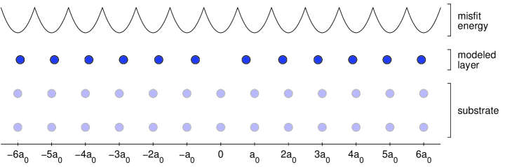
Figure 1. Frenkel-Kontorova model. The wells depict the misfit energy, $\mathcal{E}^{m,a}_{i}$.

Next, the continuum energy

$$\mathcal{E}^{c}_{i}=\mathcal{E}^{c,e}_{i}+\mathcal{E}^{c,m}_{i}$$ (2.5)

for each atom $i$ is derived from the atomistic energy, which leads to

$$\begin{split}\mathcal{E}^{c,e}_{i}(\mathbf{y})&={\textstyle\frac{1}{4}}k_{12}(y_{i}-y_{i-1}-a_{0})^{2}+{\textstyle\frac{1}{4}}k_{12}(y_{i+1}-y_{i}-a_{0})^{2},\\ \mathcal{E}^{c,m}_{i}(\mathbf{y})&=\begin{cases}{\textstyle\frac{1}{2}}k_{0}\left(y_{i}-(i-1)a_{0}\right)^{2},&i=-M+1,\ldots,0,\\ {\textstyle\frac{1}{2}}k_{0}\left(y_{i}-ia_{0}\right)^{2},&i=1,\ldots,M,\end{cases}\end{split}$$ (2.6)

where $k_{12}=k_{1}+4k_{2}$, see [2] for the details. We note that $\mathcal{E}^{c,e}_{i}(\mathbf{y})=\mathcal{E}^{a,e}_{i}(\mathbf{y})$ if $y_{i+2}-y_{i+1}=y_{i+1}-y_{i}=y_{i}-y_{i-1}=y_{i-1}-y_{i-2},$ but $\mathcal{E}^{c,e}_{i}(\mathbf{y})\neq\mathcal{E}^{a,e}_{i}(\mathbf{y})$ more generally.

For each atom $i$, we decide whether this atom is modeled atomistically or as continuum. An a posteriori error estimator for this task has been derived in [2]. Let

$$\delta_{i}^{a}=\begin{cases}1&\text{if atom $i$ is modeled atomistically,}\\ 0&\text{if atom $i$ is modeled as continuum,}\end{cases}\qquad\text{and}\qquad\delta_{i}^{c}=1-\delta_{i}^{a}.$$ (2.7)

We define the atomistic-continuum energy to be

$$\mathcal{E}^{ac}(\mathbf{y}):=\sum_{i=-M+1}^{M}\delta^{a}_{i}\mathcal{E}^{a}_{i}(\mathbf{y})+\sum_{i=-M+1}^{M}\delta^{c}_{i}\mathcal{E}^{c}_{i}(\mathbf{y}).$$ (2.8)

The next step is to coarsen out unnecessary atoms within the continuum region. This way, we restrict the system to the remaining atoms, called the representative atoms, or briefly repatoms. An a posteriori error estimator to determine the optimal coarsening will be developed in this paper. Let $\ell_{j}$ for $j=-N+1,\ldots,N$ be the index of the $j$-th repatom, where $2N$ is the number of repatoms. We require that

$$\ell_{-N+1}<\ell_{-N+2}<\cdots<\ell_{j}<\ell_{j+1}<\cdots<\ell_{N-1}<\ell_{N}$$ (2.9)

and

$$\ell_{-N+1} =-M+1, \ell_{-N+2} =-M+2, \ell_{N-1} =M-1, \ell_{N} =M.$$ (2.10)

Then

$$\nu_{j}:=\ell_{j+1}-\ell_{j}$$ (2.11)

gives the number of atomistic intervals between the repatoms $j$ and $j+1$. We denote the vector of repatoms by $\mathbf{y}^{qc}$.

The quasicontinuum energy is obtained by implicitly reconstructing the missing atoms from the repatoms by piecewise linear interpolation, and then computing the atomistic-continuum energy from the reconstructed vector. The piecewise linear interpolation can be written as the matrix multiplication $I^{aq}\mathbf{y}^{qc}$, where

$$I^{aq}_{\ell_{j}+k,j}:=\frac{\nu_{j}-k}{\nu_{j}},\qquad I^{aq}_{\ell_{j}+k,j+1}:=\frac{k}{\nu_{j}}$$ (2.12)

for $j=-N+1,\ldots,N$ and $k=0,\ldots,\nu_{j}$, and $I^{aq}_{i,j}=0$ otherwise. Hence, the quasicontinuum energy is given by

$$\mathcal{E}^{qc}(\mathbf{y}^{qc}):=\mathcal{E}^{ac}(I^{aq}\mathbf{y}^{qc}).$$ (2.13)

Summation formulas for an efficient computation of $\mathcal{E}^{qc}(\mathbf{y}^{qc})$ without having to explicitly reconstruct the non-repatoms have been derived in [2].

We describe boundary conditions at the two leftmost atoms and the two rightmost atoms. We take into account two instead of one atom at each end of the chain because of the NNN interactions. For the fully atomistic system and the atomistic-continuum system, the boundary conditions read as

$$y^{a}_{-M+1} =y^{bc}_{l1}, \qquad y^{a}_{-M+2} =y^{bc}_{l2}, \qquad y^{a}_{M-1} =y^{bc}_{r2}, \qquad y^{a}_{M} =y^{bc}_{r1},$$ (2.14)

$$y^{ac}_{-M+1} =y^{bc}_{l1}, y^{ac}_{-M+2} =y^{bc}_{l2}, y^{ac}_{M-1} =y^{bc}_{r2}, y^{ac}_{M} =y^{bc}_{r1},$$

for given values $y^{bc}_{l1}$, $y^{bc}_{l2}$, $y^{bc}_{r2}$, and $y^{bc}_{r1}$, and similarly the boundary conditions for the quasicontinuum system are given by

$$y^{qc}_{-N+1} =y^{bc}_{l1}, \qquad y^{qc}_{-N+2} =y^{bc}_{l2}, \qquad y^{qc}_{N-1} =y^{bc}_{r2}, \qquad y^{qc}_{N} =y^{bc}_{r1}.$$ (2.15)

Next, we introduce the solution spaces

$$V^{a} :={\mathbb{R}}^{2M}, \qquad V^{a}_{0} :={\mathbb{R}}^{2M-4}, \qquad V^{q} :={\mathbb{R}}^{2N}, \qquad V^{q}_{0} :={\mathbb{R}}^{2N-4}$$ (2.16)

and the boundary operators

$$J^{a}:V^{a}_{0}\to V^{a}\qquad\text{and}\qquad J^{q}:V^{q}_{0}\to V^{q}$$ (2.17)

by

$$J^{a}_{i,j} :=\delta_{ij} \quad\text{for}\quad i =-M+1,\ldots,M, j =-M+3,\ldots,M-2,$$ (2.18)

$$J^{q}_{i,j} :=\delta_{ij} \quad\text{for}\quad i =-N+1,\ldots,N, j =-N+3,\ldots,N-2.$$

$V^{a}$ and $V^{a}_{0}$ are the suitable spaces for the atomistic system and the atomistic-continuum system, both with and without boundary values, whereas $V^{q}$ and $V^{q}_{0}$ are the suitable spaces for the quasicontinuum system. $J^{a}$ and $J^{q}$ extend vectors from $V^{a}_{0}$ and $V^{q}_{0}$, respectively, by zero boundary values. Note that the interpolation operator $I^{aq}$ maps $V^{q}$ to $V^{a}$. The spaces and their operators are illustrated in Figure 2.

To implement the boundary conditions, we define the vectors

$$\mathbf{y}^{bcq} :=\begin{bmatrix}y^{bc}_{l1}&y^{bc}_{l2}&0&\cdots&0&y^{bc}_{r2}&y^{bc}_{r1}\end{bmatrix}^{T}\in V^{q},$$ (2.19)

$$\mathbf{y}^{bca} :=I^{aq}\mathbf{y}^{bcq}\in V^{a}.$$

Figure 2. Solution spaces and their operators for the fully-atomistic level (a) and the quasicontinuum level (q).

We seek minimizers of the three different potential energies subject to the boundary conditions described above, that is, vectors

$$\mathbf{\bar{y}}^{a}\in J^{a}V^{a}_{0}+\mathbf{y}^{bca}\subset V^{a},\quad\mathbf{\bar{y}}^{ac}\in J^{a}V^{a}_{0}+\mathbf{y}^{bca}\subset V^{a},\quad\text{and}\quad\mathbf{\bar{y}}^{qc}\in J^{q}V^{q}_{0}+\mathbf{y}^{bcq}\subset V^{q}$$ (2.20)

which minimize the potential energies $\mathcal{E}^{a}$, $\mathcal{E}^{ac}$, and $\mathcal{E}^{qc}$, respectively. If we decompose

$$\mathbf{\bar{y}}^{a}=J^{a}\mathbf{y}^{a}+\mathbf{y}^{bca},\qquad\mathbf{\bar{y}}^{ac}=J^{a}\mathbf{y}^{ac}+\mathbf{y}^{bca},\qquad\text{and}\qquad\mathbf{\bar{y}}^{qc}=J^{q}\mathbf{y}^{qc}+\mathbf{y}^{bcq},$$ (2.21)

then the fully atomistic solution $\mathbf{y}^{a}\in V^{a}_{0}$, the atomistic-continuum solution $\mathbf{y}^{ac}\in V^{a}_{0},$ and the quasicontinuum solution $\mathbf{y}^{qc}\in V^{q}_{0}$ are characterized by

$$\mathbf{y}^{a} =\operatorname*{arg\,min}_{\mathbf{y}\in V^{a}_{0}}\mathcal{E}^{a}(J^{a}\mathbf{y}+{\mathbf{y}}^{bca}),$$ (2.22)

$$\mathbf{y}^{ac} =\operatorname*{arg\,min}_{\mathbf{y}\in V^{a}_{0}}\mathcal{E}^{ac}(J^{a}\mathbf{y}+{\mathbf{y}}^{bca}),$$

$$\mathbf{y}^{qc} =\operatorname*{arg\,min}_{\mathbf{y}\in V^{q}_{0}}\mathcal{E}^{qc}(J^{q}\mathbf{y}+{\mathbf{y}}^{bcq}).$$

Next, we write the energies in matrix notation as

$$\mathcal{E}^{a}(\mathbf{y}) ={\textstyle\frac{1}{2}}(\mathbf{y}-\mathbf{a}^{a})^{T}D^{T}E^{a}D(\mathbf{y}-\mathbf{a}^{a})+{\textstyle\frac{1}{2}}(\mathbf{y}-\mathbf{b}^{a})^{T}K(\mathbf{y}-\mathbf{b}^{a}),$$ (2.23)

$$\mathcal{E}^{ac}(\mathbf{y}) ={\textstyle\frac{1}{2}}(\mathbf{y}-\mathbf{a}^{a})^{T}D^{T}E^{ac}D(\mathbf{y}-\mathbf{a}^{a})+{\textstyle\frac{1}{2}}(\mathbf{y}-\mathbf{b}^{a})^{T}K(\mathbf{y}-\mathbf{b}^{a}),$$

$$\mathcal{E}^{qc}(\mathbf{y}) ={\textstyle\frac{1}{2}}(I^{aq}\mathbf{y}-\mathbf{a}^{a})^{T}D^{T}E^{ac}D(I^{aq}\mathbf{y}-\mathbf{a}^{a})+{\textstyle\frac{1}{2}}(I^{aq}\mathbf{y}-\mathbf{b}^{a})^{T}K(I^{aq}\mathbf{y}-\mathbf{b}^{a}).$$

We refer to [2] for the precise and lengthy definitions of the respective matrices. In matrix notation, the vectors $\mathbf{y}^{a}$, $\mathbf{y}^{ac}$, and $\mathbf{y}^{qc}$ are the solutions of the linear systems

$$M^{a}\mathbf{y}^{a} =\mathbf{f}^{a},$$ (2.24)

$$M^{ac}\mathbf{y}^{ac} =\mathbf{f}^{ac},$$

$$M^{qc}\mathbf{y}^{qc} =\mathbf{f}^{qc},$$

where the matrices $M^{a}$, $M^{ac}$, and $M^{qc}$ are given by

$$\begin{split}M^{a}&:=J^{a^{T}}(D^{T}E^{a}D+K)J^{a},\\ M^{ac}&:=J^{a^{T}}(D^{T}E^{ac}D+K)J^{a},\\ M^{qc}&:=J^{q^{T}}I^{aq^{T}}(D^{T}E^{ac}D+K)I^{aq}J^{q},\\ \end{split}$$ (2.25)

and where the right-hand sides $\mathbf{f}^{a}$, $\mathbf{f}^{ac}$, and $\mathbf{f}^{qc}$ are defined as

$$\begin{split}\mathbf{f}^{a}&:=-J^{a^{T}}D^{T}E^{a}D(\mathbf{y}^{bca}-\mathbf{a}^{a})-J^{a^{T}}K(\mathbf{y}^{bca}-\mathbf{b}^{a}),\\ \mathbf{f}^{ac}&:=-J^{a^{T}}D^{T}E^{ac}D(\mathbf{y}^{bca}-\mathbf{a}^{a})-J^{a^{T}}K(\mathbf{y}^{bca}-\mathbf{b}^{a}),\\ \mathbf{f}^{qc}&:=-J^{q^{T}}I^{aq^{T}}D^{T}E^{ac}D(I^{aq}\mathbf{y}^{bcq}-\mathbf{a}^{a})-J^{q^{T}}I^{aq^{T}}K(I^{aq}\mathbf{y}^{bcq}-\mathbf{b}^{a}).\end{split}$$ (2.26)

3. Goal-Oriented Error Estimation

We estimate the error $\mathbf{y}^{a}-J^{a^{T}}I^{aq}J^{q}\mathbf{y}^{qc}$ in terms of a user-definable goal function

$$Q:V^{a}_{0}\to{\mathbb{R}},$$ (3.1)

that is, we aim at estimating

$$|Q(\mathbf{y}^{ac})-Q(J^{a^{T}}I^{aq}J^{q}\mathbf{y}^{qc})|.$$ (3.2)

We assume that $Q$ is linear. Hence there exists some vector $\mathbf{q}\in V^{a}_{0}$ such that

$$Q(\mathbf{y})=\mathbf{q}^{T}\mathbf{y}\qquad\forall\mathbf{y}\in V^{a}_{0}.$$ (3.3)

We decompose the error (3.3) as follows:

$$|Q(\mathbf{y}^{a})-Q(J^{a^{T}}I^{aq}J^{q}\mathbf{y}^{qc})| =|Q(\mathbf{y}^{a}-\mathbf{y}^{ac})+Q(\mathbf{y}^{ac}-J^{a^{T}}I^{aq}J^{q}\mathbf{y}^{qc})|$$ (3.4)

$$\leq|Q(\mathbf{y}^{a}-\mathbf{y}^{ac})|+|Q(\mathbf{y}^{ac}-J^{a^{T}}I^{aq}J^{q}\mathbf{y}^{qc})|$$

$$=|Q(\mathbf{e}^{a-ac})|+|Q(\mathbf{e}^{ac-qc})|$$

where

$$\mathbf{e}^{a-ac} :=\mathbf{y}^{a}-\mathbf{y}^{ac},$$ (3.5)

$$\mathbf{e}^{ac-qc} :=\mathbf{y}^{ac}-J^{a^{T}}I^{aq}J^{q}\mathbf{y}^{qc}.$$

The first term $|Q(\mathbf{e}^{a-ac})|$ constitutes the modeling error and has been treated in [2]. The second term $|Q(\mathbf{e}^{ac-qc})|$ describes the error due to mesh coarsening and will be treated in the following.

To facilitate the error analysis, we define the dual problems

$$M^{ac}\mathbf{g}^{ac} =\mathbf{q},$$ (3.6)

$$M^{qc}\mathbf{g}^{qc} =J^{q^{T}}I^{aq^{T}}J^{a}\mathbf{q}.$$

We then have the basic dual identity for the goal-oriented error

$$\begin{split}Q(\mathbf{e}^{ac-qc})&=\mathbf{q}^{T}(\mathbf{y}^{ac}-J^{a^{T}}I^{aq}J^{q}\mathbf{y}^{qc})\\ &=\mathbf{g}^{ac^{T}}M^{ac}(\mathbf{y}^{ac}-J^{a^{T}}I^{aq}J^{q}\mathbf{y}^{qc})\\ &=\mathbf{g}^{ac^{T}}{\mathcal{R}}^{ac}(J^{a^{T}}I^{aq}J^{q}\mathbf{y}^{qc})\end{split}$$ (3.7)

with the primal residual given by

$${\mathcal{R}}^{ac}(\mathbf{y}):=\mathbf{f}^{ac}-M^{ac}\mathbf{y}.$$ (3.8)

However, this quantity is too expensive to compute. We cannot solve for the dual solution $\mathbf{g}^{ac}$ on the atomistic scale, since this has the same computational complexity as solving for the uncoarsened solution $\mathbf{y}^{ac}$. To overcome this obstacle, we replace $\mathbf{g}^{ac}$ by a dual solution from a coarser space.

A first idea would be to use $J^{a^{T}}I^{aq}J^{q}\mathbf{g}^{qc}$ instead of $\mathbf{g}^{ac}$. However, this turns out to be useless due to Galerkin orthogonality:

Lemma 3.1 (Garlerkin Orthogonality).

We have

$$J^{q^{T}}I^{aq^{T}}J^{a}M^{ac}(\mathbf{y}^{ac}-J^{a^{T}}I^{aq}J^{q}\mathbf{y}^{qc})=0,$$ (3.9)

or equivalently

$$J^{q^{T}}I^{aq^{T}}J^{a}{\mathcal{R}}^{ac}(J^{a^{T}}I^{aq}J^{q}\mathbf{y}^{qc})=0.$$ (3.10)

Proof.

Multiplying the equation for $\mathbf{y}^{ac}$ from (2.24) by $J^{q^{T}}I^{aq^{T}}J^{a}$ from the left gives

$$J^{q^{T}}I^{aq^{T}}J^{a}M^{ac}\mathbf{y}^{ac}=J^{q^{T}}I^{aq^{T}}J^{a}\mathbf{f}^{ac}.$$ (3.11)

It is easy to see that

$$J^{a}J^{a^{T}}I^{aq}J^{q}=I^{aq}J^{q}.$$ (3.12)

Applying this to the equation for $\mathbf{y}^{qc}$ from (2.24) leads to

$$J^{q^{T}}I^{aq^{T}}J^{a}M^{ac}J^{a^{T}}I^{aq}J^{q}\mathbf{y}^{qc}=\mathbf{f}^{qc}.$$ (3.13)

Subtracting (3.13) from (3.11), substituting the definitions (2.26) of $\mathbf{f}^{ac}$ and $\mathbf{f}^{qc}$ and using (3.12) and (2.19) gives

$$\begin{split}J^{q^{T}}I^{aq^{T}}&J^{a}M^{ac}(\mathbf{y}^{ac}-J^{a^{T}}I^{aq}J^{q}\mathbf{y}^{qc})\\ &=J^{q^{T}}I^{aq^{T}}J^{a}\mathbf{f}^{ac}-\mathbf{f}^{qc}\\ &=J^{q^{T}}I^{aq^{T}}J^{a}J^{a^{T}}\left[-D^{T}E^{ac}D(\mathbf{y}^{bc}-\mathbf{a}^{a})-K(\mathbf{y}^{bc}-\mathbf{b}^{a})\right]\\ &\qquad-J^{q^{T}}I^{aq^{T}}\left[-D^{T}E^{ac}D(I^{aq}\mathbf{y}^{bcq}-\mathbf{a}^{a})-K(I^{aq}\mathbf{y}^{bcq}-\mathbf{b}^{a})\right]\\ &=0,\end{split}$$ (3.14)

which completes the proof. ∎

Hence, replacing $\mathbf{g}^{ac}$ in (3.7) by $J^{a^{T}}I^{aq}J^{q}\mathbf{g}^{qc}$ always gives a zero estimate for the goal-oriented error. We need to use the dual solution from some space which is finer than $V^{q}_{0}$ to get a non-zero estimate for the goal-oriented error, but which is coarser than $V^{a}_{0}$ to make it computable.

To this end, we introduce an additional level of refinement and denote it as the partial continuum (pc) level. Similarly to the repatoms on the qc-level, we chose a set of $2\bar{N}$ pc-level repatoms which is a subset of all atoms and a superset of the qc-repatoms. This means we choose indices $\bar{\ell}_{\bar{\jmath}}$ for $\bar{\jmath}=-\bar{N}+1,\ldots,\bar{N}$ such that

$$\bar{\ell}_{-\bar{N}+1}<\bar{\ell}_{-\bar{N}+2}<\cdots<\bar{\ell}_{\bar{\jmath}}<\bar{\ell}_{\bar{\jmath}+1}<\cdots<\bar{\ell}_{\bar{N}-1}<\bar{\ell}_{\bar{N}}$$ (3.15)

and

$$\bar{\ell}_{-\bar{N}+1} =-M+1, \bar{\ell}_{-\bar{N}+2} =-M+2, \bar{\ell}_{\bar{N}-1} =M-1, \bar{\ell}_{\bar{N}} =M.$$ (3.16)

To ensure that the pc-level is actually a refinement of the qc-level, we require every qc-level repatom to be a pc-level repatom. Hence there exist indices $\mu_{j}$ such that

$$\ell_{j}=\bar{\ell}_{\mu_{j}},\qquad j=-N+1,\ldots,N.$$ (3.17)

Similar to the definition of $\nu_{j}$, we denote the number of atomistic intervals between two pc-level repatoms by

$$\bar{\nu}_{\bar{\jmath}}:=\bar{\ell}_{\bar{\jmath}+1}-\bar{\ell}_{\bar{\jmath}},\qquad\bar{\jmath}=-\bar{N}+1,\ldots,\bar{N}-1.$$ (3.18)

See Figure 3 for an illustration of the three levels of refinement and the corresponding variables.

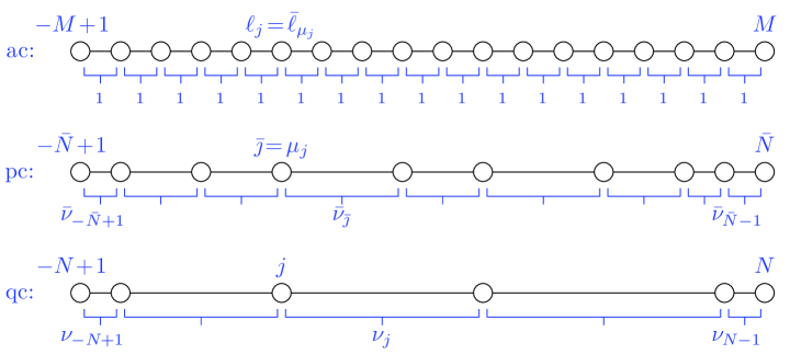
Figure 3. Levels of refinement: atomistic-continuum (ac), partial continuum (pc), and quasicontinuum (qc) with indices (above the respective chain) and intervals (below the respective chain).

We define the pc-level solution spaces

$$V^{p}:={\mathbb{R}}^{2\bar{N}}\qquad\text{and}\qquad V^{p}_{0}:={\mathbb{R}}^{2\bar{N}-4},$$ (3.19)

the interpolation operators

$$\left.\begin{aligned} I^{ap}_{\bar{\ell}_{\bar{\jmath}}+\bar{k},\bar{\jmath}}&:=\makebox[70.0001pt][l]{$\displaystyle\frac{\bar{\nu}_{\bar{\jmath}}-\bar{k}}{\bar{\nu}_{\bar{\jmath}}}$}\\ I^{ap}_{\bar{\ell}_{\bar{\jmath}}+\bar{k},\bar{\jmath}+1}&:=\makebox[70.0001pt][l]{$\displaystyle\frac{\bar{k}}{\bar{\nu}_{\bar{\jmath}}}$}\end{aligned}\quad\right\} \quad\text{for }\bar{\jmath}=-\bar{N}+1,\ldots,\bar{N}-1,\quad\bar{k}=0,\ldots,\bar{\nu}_{\bar{\jmath}},$$ (3.20)

$$I^{ap}_{i,\bar{\jmath}}:=\makebox[89.00006pt][l]{$0$} \quad\text{otherwise},$$

$$\left.\begin{aligned} I^{pq}_{\mu_{j}+k,j}&:=\makebox[70.0001pt][l]{$\displaystyle\frac{\nu_{j}-\bar{\ell}_{\mu_{j}+k}+\bar{\ell}_{\mu_{j}}}{\nu_{j}}$}\\ I^{pq}_{\mu_{j}+k,j+1}&:=\makebox[70.0001pt][l]{$\displaystyle\frac{\bar{\ell}_{\mu_{j}+k}-\bar{\ell}_{\mu_{j}}}{\nu_{j}}$}\end{aligned}\quad\right\} \quad\text{for }j=-N+1,\ldots,N-1,\quad k=0,\ldots,\mu_{j+1}-\mu_{j},$$

$$I^{pq}_{\bar{\jmath},j}:=\makebox[89.00006pt][l]{$0$} \quad\text{otherwise},$$

the restriction operator

$$R^{qp}_{j,\bar{\jmath}} :=\delta_{\mu_{j},\bar{\jmath}}\qquad\text{for}\quad j=-N+1,\ldots,N,\quad\bar{\jmath}=-\bar{N}+1,\ldots,\bar{N},$$ (3.21)

and the boundary operator

$$J^{p}_{i,j} :=\delta_{ij}\qquad\text{for}\quad i=-\bar{N}+1,\ldots,\bar{N},\quad j=-\bar{N}+3,\ldots,\bar{N}-2.$$ (3.22)

Note that the interpolation operators are defined in such a way that $I^{aq}$ factors as

$$I^{aq}=I^{ap}I^{pq}.$$ (3.23)

Altogether, all solution spaces and the corresponding operators are depicted in Figure 4.

(3.30)

Figure 4. Solution spaces and their operators for the ac-level, pc-level, and qc-level.

We solve the dual equation on the newly introduced partial continuum level:

$$M^{pc}\mathbf{g}^{pc} =J^{p^{T}}I^{ap^{T}}J^{a}\mathbf{q},$$ (3.31)

where

$$M^{pc} :=J^{p^{T}}I^{ap^{T}}(D^{T}E^{ac}D+K)I^{ap}J^{p}.$$ (3.32)

We use $\mathbf{g}^{pc}$ to get an approximation of the goal-oriented error:

$$Q(\mathbf{y}^{ac})-Q(J^{a^{T}}I^{aq}J^{q}\mathbf{y}^{qc})\approx\mathbf{g}^{pc^{T}}J^{p^{T}}I^{ap^{T}}J^{a}{\mathcal{R}}^{ac}(J^{a^{T}}I^{aq}J^{q}\mathbf{y}^{qc}).$$ (3.33)

Due to Galerkin Orthogonality (Lemma 3.1), we can subtract any vector in $V^{q}_{0}$ from the right hand side expression without changing its value. Thus, we subtract from $\mathbf{g}^{pc}$ the linear interpolation of the nodal values of $\mathbf{g}^{pc}$ at the qc-repatoms, $J^{p^{T}}I^{pq}R^{qp}J^{p}\mathbf{g}^{pc}$, to get a vector in $V^{p}_{0}$ that is zero at the qc-repatoms. This leads us to the error estimator

$$\begin{split}\eta:=&\>\big{[}\mathbf{g}^{pc}-J^{p^{T}}I^{pq}R^{qp}J^{p}\mathbf{g}^{pc}\big{]}^{T}J^{p^{T}}I^{aq^{T}}J^{a}{\mathcal{R}}^{ac}(J^{a^{T}}I^{aq}J^{q}\mathbf{y}^{qc})\\ =&\>\big{[}\mathbf{g}^{pc}-J^{p^{T}}I^{pq}R^{qp}J^{p}\mathbf{g}^{pc}\big{]}^{T}\big{[}J^{p^{T}}I^{aq^{T}}J^{a}\mathbf{f}^{ac}-M^{pc}\mathbf{y}^{pc}\big{]}\end{split}$$ (3.34)

as an approximation to (3.7).

In Section 5, we will construct a numerical method based on this error estimator. We will then compute numerically how much the approximation (3.34) deviates from the precise error (3.7), and we will determine how fine the partial refinement needs to be.

4. Numerical Method

Based on the error estimator $\eta$, we need to decide what intervals at the qc-level shall be refined. To this end, we split $\eta$ into individual contributions from each pc-level repatom:

$$\eta=\sum_{\bar{\jmath}=-\bar{N}+3}^{\bar{N}-2}\eta^{pc}_{\bar{\jmath}}$$ (4.1)

where

$$\eta^{pc}_{\bar{\jmath}}:=\big{[}\mathbf{g}^{pc}-J^{p^{T}}I^{pq}R^{qp}J^{p}\mathbf{g}^{pc}\big{]}_{\bar{\jmath}}\big{[}J^{p^{T}}I^{aq^{T}}J^{a}{\mathcal{R}}^{ac}(J^{a^{T}}I^{aq}J^{q}\mathbf{y}^{qc})\big{]}_{\bar{\jmath}}.$$ (4.2)

Next, we map the values $\eta^{pc}_{\bar{\jmath}}$ to the qc-level intervals. Note that we already have $\eta^{pc}_{\bar{\jmath}}=0$ whenever $\bar{\jmath}$ is a qc-repatom because we subtracted the qc-level interpolant from $\mathbf{g}^{pc}$ in (3.34). We accumulate the remaining values $\eta^{pc}_{\bar{\jmath}}$ to the interval between the qc-repatoms $j$ and $j+1$ if the pc-repatom ${\bar{\jmath}}$ lies between the qc-repatoms $j$ and $j+1$, that is, $\mu_{j}<{\bar{\jmath}}<\mu_{j+1},$ to obtain

$$\eta^{qc}_{j}:=\Bigg{|}\sum_{\bar{\jmath}=\mu_{j}+1}^{\mu_{j+1}-1}\eta^{pc}_{\bar{\jmath}}\Bigg{|}.$$ (4.3)

Moreover, we have to decide how to compute the partial refinement. Here we subdivide each qc-interval $(\ell_{j},\ell_{j+1})$ into a fixed number $\Lambda$ of subintervals of the same size, although other strategies are possible, like letting $\Lambda$ depend on the respective interval size $\nu_{j}=\ell_{j+1}-\ell_{j}$, or dividing each interval into subintervals of different sizes. But here we stick to a fixed number $\Lambda\in{\mathbb{N}}$ and an equidistant subdivision. We employ the following algorithm for partial refinement:

$\bar{\jmath}\leftarrow-\bar{N}+1$
                  for $j=-N+1,\ldots,N-1$
                           $\omega\leftarrow\max(1,\nu_{j}/\Lambda$)
                           $\sigma_{1}\leftarrow 0$
                           $\sigma_{2}\leftarrow 0$
                           while $(\sigma_{2}<\nu_{j})$
                                    $\sigma_{1}\leftarrow\min(\sigma_{1}+\omega,\nu_{j})$
                                    $\bar{\nu}_{\bar{\jmath}}\leftarrow\lfloor\sigma_{1}-\sigma_{2}+{\textstyle\frac{1}{2}}\rfloor$
                                    $\sigma_{2}\leftarrow\sigma_{2}+\bar{\nu}_{\bar{\jmath}}$
                                    $\bar{\jmath}\leftarrow\bar{\jmath}+1$
                           end
                  end

Note that this algorithm performs the necessary rounding if $\nu_{j}$ is not divisible by $\Lambda$. If $\nu_{j}\leq\Lambda$, then the interval gets fully refined up to the atomistic level.

We then use this partial refinement algorithm and the global and local error estimators above to construct the following algorithm for adaptive mesh coarsening:

1. Start with the model fully coarsened in the continuum region.

2. Solve the primal problem (2.24) for $\mathbf{y}^{qc}.$

3. Determine the partial refinement pc according to the algorithm above.

4. Solve the dual problem (3.31) for $\mathbf{g}^{pc}$.

5. Compute the global error estimator $\eta$ from (3.34).

6. If $\eta\leq\tau_{gl}$, then stop.

7. Compute the local error estimators $\eta^{qc}_{j}$ from (4.2) and (4.3).

8. Refine all intervals $(j,j+1)$ with

   $$\eta^{qc}_{j}\geq\frac{1}{\tau_{fac}}\max_{k}\eta^{qc}_{k}$$ (4.4)

   into two subintervals.

9. Go to (2).

Here $\tau_{gl}>0$ denotes the global error tolerance. For the adaption criterion (4.4), numerical evidence has shown that $\tau_{fac}=10$ is a reasonable choice.

A possible improvement of step (8) would be to use the absolute value of the error estimator $\eta^{qc}_{j}$ to decide into how many subintervals each interval $(j,j+1)$ shall be refined, instead of just refining into two subintervals. However, the magnitudes of the values $\eta^{qc}_{j}$ differ considerably only in the first iterations. So this would only eliminate some of the early iterations which are still cheap due to the small number of unknowns involved there, whereas the computationally expensive later iterations will not be affected. Hence we expect the overall speedup to be small.

5. Numerical Results

Now we present and discuss our numerical results. We choose boundary conditions

$$y^{bc}_{l1}=-M,\qquad y^{bc}_{l2}=-M+1,\qquad y^{bc}_{r2}=M-1,\qquad y^{bc}_{r1}=M.$$ (5.1)

The elastic moduli are given by $k_{0}=0.1$, $k_{1}=2$, and $k_{2}=1$, and the lattice constant is $a_{0}=1$.

We consider a chain of 4106 atoms, that is $M=2053$. There is an atomistic region of $4$ atoms from $-1$ to $2$ around the dislocation at the center of the chain. The remaining part is modeled as continuum. We set atoms $-3,\,-2,\,3,\,4$ to be continuum repatoms so that $\mathcal{E}^{a}_{-1}(I^{aq}\mathbf{y}^{qc})$ and $\mathcal{E}^{a}_{2}(I^{aq}\mathbf{y}^{qc})$ can be evaluated without interpolation, and we set and atoms $-M+1,\,-M+2,\,M-1,\,M$ to be continuum repatoms so that the boundary conditions can be set. Initially, the mesh in the continuum region is maximally coarsened, so that there are no more repatoms in addition to the ones already mentioned. This gives $N=6$ and 12 qc-level degrees of freedom. There are two large elements of size $\nu_{-4}=\nu_{4}=2048$, one on each side of the dislocation at the center of the chain, whereas the remaining elements necessarily have sizes $\nu_{j}=1$ for $j=-5,-3,-2,-1,0,1,2,3,5$. The mesh is shown in the upper graph of Figure 5.

The quantity of interest here is the size $y_{1}-y_{0}$ of the dislocation at the center of the chain, that is, the distance between the two atoms 0 and 1 to the left and right of the dislocation. The corresponding vector $\mathbf{q}\in V^{a}_{0}$ reads as

$$\mathbf{q}=[0,\ldots,0,-1,1,0,\ldots,0]^{T}.$$ (5.2)

iteration	#dof	$\min\nu_{j}$	$\max\nu_{j}$	$\eta$	$\sum_{j=-N+1}^{N-1}\eta_{j}^{qc}$	$|Q(\mathbf{e}^{ac-qc})|$
1	12	2048	2048	3.143618e-03	3.143618e-03	6.777614e-02
2	14	1024	1024	5.208032e-03	5.443530e-03	6.463252e-02
3	16	512	1024	8.771892e-03	9.133002e-03	5.946329e-02
4	18	256	1024	1.293987e-02	1.343519e-02	5.074706e-02
5	20	128	1024	1.520764e-02	1.565599e-02	3.787477e-02
6	22	64	1024	1.267077e-02	1.279361e-02	2.271288e-02
7	24	32	1024	6.760509e-03	6.767672e-03	1.004707e-02
8	26	16	1024	2.395699e-03	2.395699e-03	3.286644e-03
9	28	8	1024	6.933383e-04	6.933394e-04	9.216477e-04
10	32	4	1024	2.061976e-04	2.061988e-04	2.638938e-04
11	40	2	1024	5.841551e-05	5.841804e-05	6.391755e-05
12	54	1	1024	7.567732e-06	7.570401e-06	9.376934e-06

Table 1. Advance of the algorithm until the error tolerance $\tau_{gl}=10^{-5}$ is achieved.

Table 1 shows how the algorithm proceeds for an error tolerance of $\tau_{gl}=10^{-5}$. One can easily see how the elements get refined and the error drops. Also shown is the precise error $|Q(\mathbf{e}^{ac-qc})|$ which is available for this small model problem. Note that the column $\min\nu_{j}$ refers only to the elements in the continuum region which actually can be coarsened, excluding the padding around the atomistic region and the boundary layer.

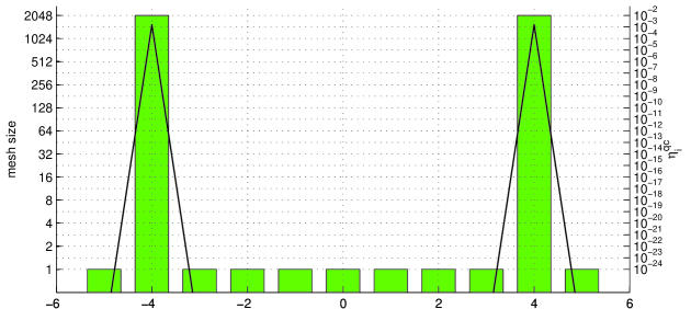
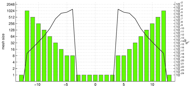
Figure 5. Mesh size $\nu_{j}$ (green bar graph) and $\eta^{qc}_{j}$ (black line graph) for error tolerances $\tau_{gl}=10^{-1}$ (top), $\tau_{gl}=10^{-3}$ (middle) and $\tau_{gl}=10^{-5}$ (bottom).

The bar graph in Figure 5 shows the size of the individual elements in the meshes before the first iteration and after the error tolerances $\tau_{gl}=10^{-3}$ and $\tau_{gl}=10^{-5}$ are achieved. One can clearly see how the elements get successively refined towards the center.

The black lines in Figure 5 depict the decomposed error estimator $\eta^{qc}_{j}$. As a result of the Galerkin orthogonality, it vanishes whereever the mesh is fully refined up to the atomistic level. We can as well read off the graphs how the algorithm tends to distribute the error uniformly over the whole mesh as the error tolerance is decreased. For $\tau_{gl}=10^{-5}$, we already achieved a close to flat region from elements $-20\ldots-13$ and $13\ldots 20$.

	$|Q(\mathbf{e}^{ac-qc})|$	$\Lambda$	$\eta$	$\sum\eta^{qc}_{j}$	$\eta/|Q(\mathbf{e}^{ac-qc})|$	$\sum\eta^{qc}_{j}/|Q(\mathbf{e}^{ac-qc})|$
mesh 1	6.777614e-02	2	3.143618e-03	3.143618e-03	0.046382	0.046382
		4	8.351650e-03	8.351650e-03	0.123224	0.123224
		8	1.708501e-02	1.708501e-02	0.252080	0.252080
		$\infty$	6.777614e-02	6.777614e-02	1.000000	1.000000
mesh 2	9.216477e-04	2	6.933383e-04	6.933394e-04	0.752281	0.752282
		4	8.749195e-04	8.749264e-04	0.949299	0.949307
		8	9.208978e-04	9.209073e-04	0.999186	0.999197
		$\infty$	9.216477e-04	9.216582e-04	1.000000	1.000011
mesh 3	9.376934e-06	2	7.567732e-06	7.570401e-06	0.807058	0.807343
		4	9.070422e-06	9.085687e-06	0.967312	0.968940
		8	9.320553e-06	9.341074e-06	0.993987	0.996176
		$\infty$	9.376934e-06	9.399414e-06	1.000000	1.002397

Table 2. Efficiency of the error estimator, $\eta$.

Table 2 shows the efficiency of the error estimator for different meshes and different values of $\Lambda$. Meshes 1, 2, and 3 refer to the meshes displayed in Figure 5. For comparison, we also include the value $\Lambda=\infty$, which indicates that the pc-level mesh for the dual solution is fully refined to the atomistic level. One can read off from this table that the error indicator gets closer to the precise error if the mesh gets finer. For the coarse mesh 1, the actual error is considerably underestimated. However, this has only little impact on the final mesh since all elements have to be refined anyhow. For the finer meshes 2 and 3, $\eta$ gets closer to the precise error $|Q(\mathbf{e}^{ac-qc})|$.

Also, we can see from Table 2 how the choice of $\Lambda$ affects the error estimator. As expected, $\eta$ gets closer to the precise error the larger $\Lambda$ gets. For computational efficiency, we are interested in keeping $\Lambda$ small, though. We can read off from the table for the fine mesh 3 that already the smallest possible value $\Lambda=2$ gives a good estimate of the error, with a deviation of less than 20%. For $\Lambda=4$, we already get a very precise estimate.

The absolute accuracy of the error estimator is important, but even more important is how well $\eta$ controls the mesh refinement, that is how efficient the resulting mesh is in terms of reaching a prescribed error tolerance with a minimal number of degrees of freedom. We now investigate the influence of the parameter $\Lambda$ on the mesh quality.

	$\Lambda=2$					$\Lambda=4$	$\Lambda=8$	$\Lambda=\infty$
it	#dof	$|Q(\mathbf{e}^{ac-qc})|$	$\eta$	#dof	$|Q(\mathbf{e}^{ac-qc})|$	$\eta$	$\eta$	$\eta$
1	12	6.778e-02	3.144e-03	12	6.778e-02	8.352e-03	1.709e-02	6.778e-02
2	14	6.463e-02	5.208e-03	14	6.463e-02	1.394e-02	2.683e-02	6.463e-02
3	16	5.946e-02	8.772e-03	16	5.946e-02	2.166e-02	3.680e-02	5.946e-02
4	18	5.075e-02	1.294e-02	18	5.075e-02	2.808e-02	4.070e-02	5.075e-02
5	20	3.787e-02	1.521e-02	20	3.787e-02	2.783e-02	3.459e-02	3.787e-02
6	22	2.271e-02	1.267e-02	22	2.271e-02	1.943e-02	2.182e-02	2.271e-02
7	24	1.005e-02	6.761e-03	24	1.005e-02	9.157e-03	9.830e-03	1.005e-02
8	26	3.287e-03	2.396e-03	26	3.287e-03	3.069e-03	3.243e-03	3.287e-03
9	28	9.216e-04	6.933e-04	28	9.216e-04	8.749e-04	9.209e-04	9.216e-04
10	32	2.639e-04	2.062e-04	32	2.639e-04	2.602e-04	2.631e-04	2.639e-04
11	40	6.392e-05	5.842e-05	40	6.392e-05	6.300e-05	6.386e-05	6.392e-05
12	54	9.377e-06	7.568e-06	56	7.955e-06	7.820e-06	7.943e-06	7.955e-06
13	68	1.809e-06	1.502e-06	70	1.234e-06	1.222e-06	1.234e-06	1.234e-06
14	82	3.144e-07	2.550e-07	84	1.644e-07	1.620e-07	1.641e-07	1.644e-07
15	90	8.887e-08	7.358e-08	100	2.075e-08	2.036e-08	2.069e-08	2.075e-08
16	102	1.712e-08	1.530e-08	116	3.001e-09	2.921e-09	2.986e-09	3.001e-09
17	118	2.421e-09	1.952e-09	132	4.695e-10	4.549e-10	4.666e-10	4.695e-10
18	132	4.695e-10	3.900e-10	144	9.720e-11	9.405e-11	9.715e-11	9.720e-11

Table 3. Mesh efficiency.

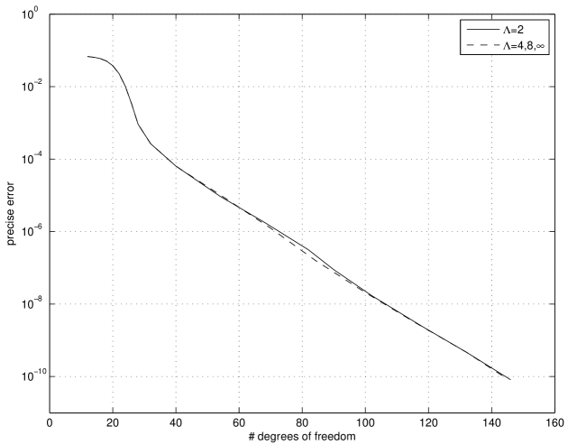
Figure 6. Mesh efficiency.

Table 3 shows the number of degrees of freedom and the corresponding error during the automatic mesh adaption for different values of $\Lambda$. The choices $\Lambda=4$, $\Lambda=8$, and $\Lambda=\infty$ lead to different values of $\eta$, but all result in the same mesh. For this reason, these values share a common column for #dof and the precise error in the table. Figure 6 visualizes the relationship between the number of degrees of freedom and the error. We can see that $\Lambda=4,8,\infty$ leads to slightly better mesh that $\Lambda=2$. However the difference is quite small so that the faster computation with $\Lambda=2$ is very well acceptable.

References

- [1] M. Ainsworth and J. T. Oden, A Posteriori Error Estimation in Finite Element Analysis, Wiley, New York, 2000.
- [2] M. Arndt and M. Luskin, Error estimation and atomistic-continuum adaptivity for the quasicontinuum approximation of a Frenkel-Kontorova model, Multiscale Model. Simul., (2007), arXiv:0704.1924. Accepted.
- [3] , Goal-oriented atomistic-continuum adaptivity for the quasicontinuum approximation, Int. J. Multiscale Comput. Eng., (2007), arXiv:0708.0025. Accepted.
- [4] S. Badia, M. L. Parks, P. B. Bochev, M. Gunzburger, and R. B. Lehoucq, On atomistic-to-continuum (AtC) coupling by blending, Technical report SAND 2007-5126J, Sandia National Laboratories, 2007.
- [5] W. Bangerth and R. Rannacher, Adaptive Finite Element Methods for Differential Equations, Lectures in Mathematics, ETH Zürich, Birkhäuser, Basel, 2003.
- [6] X. Blanc, C. Le Bris, and F. Legoll, Analysis of a prototypical multiscale method coupling atomistic and continuum mechanics, Math. Model. Numer. Anal., 39 (2005), pp. 797–826.
- [7] W. A. Curtin and R. E. Miller, Atomistic/continuum coupling in computational materials science, Modelling Simul. Mater. Sci. Eng., 11 (2003), pp. R33–R68.
- [8] M. Dobson and M. Luskin, Analysis of a force-based quasicontinuum approximation, Math. Model. Numer. Anal., (2007), arXiv:math.NA/0611543. To appear.
- [9] W. E, J. Lu, and J. Z. Yang, Uniform accuracy of the quasicontinuum method, Phys. Rev. B, 74 (2006), p. 214115.
- [10] W. E and P. Ming, Analysis of multiscale methods, J. Comput. Math., 22 (2004), pp. 210–219.
- [11] J. Knap and M. Ortiz, An analysis of the quasicontinuum method, J. Mech. Phys. Solids, 49 (2001), pp. 1899–1923.
- [12] P. Lin, Theoretical and numerical analysis for the quasi-continuum approximation of a material particle model, Math. Comput., 72 (2003), pp. 657–675.
- [13] , Convergence analysis of a quasi-continuum approximation for a two-dimensional material without defects, SIAM J. Numer. Anal., 45 (2007), pp. 313–332.
- [14] W. K. Liu, E. G. Karpov, S. Zhang, and H. S. Park, An introduction to computational nanomechanics and materials, Comput. Methods Appl. Mech. Eng., 193 (2004), pp. 1529–1578.
- [15] M. Marder, Condensed Matter Physics, John Wiley & Sons, 2000.
- [16] R. Miller and E. Tadmor, The quasicontinuum method: Overview, applications and current directions, J. Comput. Aided Mater. Des., 9 (2002), pp. 203–239.
- [17] R. Miller, E. B. Tadmor, R. Phillips, and M. Ortiz, Quasicontinuum simulation of fracture at the atomic scale, Modelling Simul. Mater. Sci. Eng., 6 (1998), pp. 607–638.
- [18] J. T. Oden, S. Prudhomme, and P. Bauman, On the extension of goal-oriented error estimation and hierarchical modeling to discrete lattice models, Comput. Methods Appl. Mech. Eng., 194 (2005), pp. 3668–3688.
- [19] , Error control for molecular statics problems, Int. J. Multiscale Comput. Eng., 4 (2006), pp. 647–662.
- [20] C. Ortner and E. Süli, A-posteriori analysis and adaptive algorithms for the quasicontinuum method in one dimension, Research Report NA-06/13, Oxford University Computing Laboratory, 2006.
- [21] , A-priori analysis of the quasicontinuum method in one dimension, Research Report NA-06/12, Oxford University Computing Laboratory, 2006.
- [22] M. L. Parks, P. B. Bochev, and R. B. Lehoucq, Connecting atomistic-to-continuum coupling and domain decomposition, Technical report SAND 2007-0704J, Sandia National Laboratories, 2007.
- [23] V. B. Shenoy, R. Miller, E. B. Tadmor, D. Rodney, R. Phillips, and M. Ortiz, An adaptive finite element approach to atomic-scale mechanics - the quasicontinuum method, J. Mech. Phys. Solids, 47 (1999), pp. 611–642.
- [24] E. B. Tadmor, M. Ortiz, and R. Phillips, Quasicontinuum analysis of defects in solids, Philos. Mag. A, 73 (1996), pp. 1529–1563.
- [25] S. P. Xiao and T. Belytschko, A bridging domain method for coupling continua with molecular dynamics, Comput. Methods Appl. Mech. Eng., 193 (2004), pp. 1645–1669.