The Hamiltonian Mean Field model: anomalous or normal diffusion?

Abstract

We consider the out-of-equilibrium dynamics of the Hamiltonian Mean Field (HMF) model, by focusing in particular on the properties of single-particle diffusion. As we shall here demonstrate analytically, if the autocorrelation of momenta in the so-called quasi-stationary states can be fitted by a $q$-exponential, then diffusion ought to be normal for $q<2$, at variance with the interpretation of the numerical experiments proposed in Ref. rapisarda .

1 Introduction

Several numerical studies have revealed that systems with long-range interactions present many interesting, and pretty unique, dynamical features which take place out-of-equilibrium, manifesting a strong sensitivity to initial conditions. To investigate these peculiar aspects and eventually develop a comprehensive theoretical framework, it is extremely valuable to dispose of a simple toy-model that admits an Hamiltonian formulation in terms of continuous variables. A paradigmatic example is represented by the so-called Hamiltonian Mean Field (HMF) model antoni-95 , which describes the evolution of $N$ particles coupled through an equally strong attractive cosine interaction. The model is specified by the following Hamiltonian:

$$H=\frac{1}{2}\sum_{j=1}^{N}p_{j}^{2}+\frac{1}{2N}\sum_{i,j=1}^{N}[1-\cos(\theta_{i}-\theta_{j})]$$ (1)

where $\theta_{i}\in[0,2\pi[$ represents the position (angle) of the $j$-th particle on a unitary radius circle and $p_{j}$ stands for its conjugate momentum. The HMF model can also be seen as a simplification of the gravitational sheet model Feix , when considering only the first harmonic in the Fourier expansion of the potential. It is exactly solvable both in the canonical and microcanonical ensembles, leading in this case to equivalent results, and displays a second order phase transitions from a homogeneous to a clustered phase when decreasing energy or temperature. The most striking observations relate however to nonequilibrium dynamics. Indeed, when performing numerical simulations starting out-of-equilibrium, the system remains trapped in long-lived Quasi Stationary States (QSSs), before relaxing to thermodynamic equilibrium. In this dynamical regime the evolution is particularly slow and the system displays non-Gaussian momentum distributionsrapisarda ; antoniazzi_prl . To monitor the evolution of the system, it is customary to introduce the magnetization, an order parameter defined as $M=|{\mathbf{M}}|=|\sum{\mathbf{m}_{i}}|/N$, where ${\mathbf{m}_{i}}=(\cos\theta_{i},\sin\theta_{i})$ is the magnetization vector. Simulations are often carried out for water-bag initial distributions, for which the one-body distribution function $f(\theta,p,t)$ takes at $t=0$ a non vanishing constant value only inside the rectangular phase-space domain $D$ specified by

$$D=\{(\theta,p)\in[-\pi,\pi]\times[-\infty,\infty]~{}|~{}|\theta|<\Delta\theta,~{}|p|<\Delta p\},$$ (2)

where $0\leq\Delta\theta\leq\pi$ and $\Delta p\geq 0$. The initial magnetization $M_{0}$ and the energy density $U$ can be expressed as functions of $\Delta\theta$ and $\Delta p$

$$M_{0}=\frac{\sin(\Delta\theta)}{\Delta\theta},\quad U=\frac{(\Delta p)^{2}}{6}+\frac{1-(M_{0})^{2}}{2}~{}.$$

This in turn implies that the initial water-bag profiles are uniquely determined by $M_{0}$ and $U$, which take values in the ranges $0\leq M_{0}\leq 1$ and $U\geq(1-M_{0}^{2})/2$.

The mean square angular displacement $\sigma^{2}(t)=\frac{1}{N}\sum_{i}{[\theta_{i}(t)-\theta_{i}(0)]^{2}}$ is also a quantity of interest. The scaling $\sigma^{2}\propto t^{\gamma}$ defines the diffusive behavior: $\gamma=1$ corresponds to normal diffusion and $\gamma=2$ to free particle ballistic dynamics. Intermediate cases correspond to the anomalous superdiffusive behavior. On the numerical simulations side, it is claimed in Ref. rapisarda that QSSs display anomalous diffusion with an exponent $\gamma$ in the range $1.4-1.5$ for $0.4\leq M_{0}\leq 1$

The same authors investigated the decay of the momentum autocorrelation functions and suggested that the numerical profiles are well interpolated by a so-called $q$-exponential function tsallis . Based on this finding, a possible relation between the fitted value $q$ and the diffusion exponent $\gamma$ has been hypothesised rapisarda .

We shall here analytically prove that the aforementioned results are contradictory. More specifically, assuming a $q$-exponential decay of the autocorrelation of momenta implies normal diffusion, for the range of values of $q$ reported in Ref. rapisarda .

Angular diffusion and momentum autocorrelation for the HMF model have been often discussed in the literature antoniazzi_prl ; latora_rapisarda_ruffo ; YAMA ; thierry . In order to provide a comprehensive picture on this subject, we will shortly review some of these contributions in the next Section. The following Section is instead devoted to presenting our analytic argument. Finally we sum up and draw our conclusions.

2 On the relation between relaxation and diffusion for the HMF model

Numerical evidence for a superdiffusive behaviour in the HMF model was first reported in latora_rapisarda_ruffo . In this paper a water-bag initial condition was assumed, with the particles positioned in $\theta_{i}=0$, a choice which corresponds to select initially the magnetized state $M_{0}=1$. It was also claimed in latora_rapisarda_ruffo that the anomalous diffusion occurs for a transient out–of–equilibrium regime, when the system is trapped in a QSS.

Successive numerical experiments YAMA carried on for a homogeneous initial distribution, i.e. $M_{0}=0$, revealed that the anomalies in diffusion are instead associated to the (nonstationary) relaxation to equilibrium. The QSS should therefore be characterized by a normal diffusive regime: it was in fact argued that the anomalous diffusion detected in latora_rapisarda_ruffo stems from finite size effects.

Motivated by such controversial findings, the authors in rapisarda set down to elucidate the role of initial conditions in driving HMF dynamical anomalies. To this end the usual water–bag initial distribution was considered, with the particles confined in a variable portion of the unitary circle, so to span the whole interval $0\leq M_{0}\leq 1$. First, the momentum autocorrelation function was introduced as:

$$C_{p}(t;0)=\langle p(t)p(0)\rangle_{N}=\frac{1}{N}\sum_{i}^{N}p_{i}(t)p_{i}(0),$$ (3)

and its decay monitored, for different values of $M_{0}$. The numerical curves were then interpolated with the $q$-exponential:

$$e_{q}(t,\tau)=[1-(1-q)t/\tau]^{\frac{1}{1-q}},$$ (4)

a function which arises in the realm of Tsallis’ generalized thermostatistics tsallis . Both $\tau$ and $q$ are numerically adjusted in rapisarda : $q$ is empirically found to be $1.5$ for $M_{0}\geq 0.4$, while it progressively diminuishes for smaller values of $M_{0}$. For $M_{0}=0$ an almost exponential decay is measured. In this respect, the homogeneous condition was assigned a special nature, and claimed to be intrinsically different from the initially magnetized configurations. This conclusion was further strengthened by looking at the diffusive properties of the system. For $M_{0}>0$, superdiffusion is systematically observed in Ref. rapisarda , while the case $M_{0}=0$ tends to a normal diffusive behavior when increasing the number of simulated particles, as previously found in YAMA . Moreover, a closed analytical relation was conjectured between the index $q$ and the diffusion exponent $\gamma$, based on an generalization of the standard Fokker-Planck equation tsa-buk . Such relation reads rapisarda ; tsa-buk :

$$\gamma=\frac{2}{3-q}$$ (5)

and returns values of $\gamma$ similar to those measured in rapisarda , when the corresponding $q$ are inserted. This supposed agreement is merely a coincidence, as we shall prove in the following. If one assumes a $q$-exponential decay for the autocorrelation of momenta, then normal diffusion is to be exptected, for the range of $q$ reported in rapisarda . Before turning to illustrate this point, we shall devote the remaining part of this Section to complete our review on the studies of diffusion for the HMF model.

Among other interesting contributions, Ref. anteneodo is worth mentioning: here the controversy on the role of the initial condition is also addressed. In particular a fully magnetized ($M_{0}=1$) initial condition is investigated. For finite sizes, a superdiffusive phase is indeed detected, in agreement with rapisarda ; latora_rapisarda_ruffo . However, the local exponent $\gamma$ is shown to converge to the normal diffusion value $\gamma=1$ as the numbers of particle is increased. Thus, anomalous diffusion is just a finite size effect, an observation which confirms the scenario proposed in YAMA for the homogeneous initial setting. A similar conclusion is also reached in antoniazzi_prl , where the time evolution of $\sigma^{2}$ is monitored by employing a larger number of particles than in previous studies. An almost normal diffusion is reported also for intermediate values of the initial magnetization.

Finally, in Ref. thierry a kinetic approach that goes beyond the Vlasov approximation was developed. This methodology enables to esplicitly calculate the momentum autocorrelation function in terms of the momentum distribution at $t=0$, namely $f_{0}(p)$. This approach applies to homogeneous initial distributions and assumes that the system is initially in a QSS. The distribution $f_{0}(p)$ with algebraic tails corresponds to a correlation function of momenta with an algebraic decay in the long time regime, hence resulting in a superdiffusive behaviour. In contrast, for distributions with Gaussian tails, $C_{p}(t;0)$ scales as $\ln t/t$, which in turn implies an approximately normal scaling for the mean–square displacement of the angles. The validity of these predictions has been recently confirmed in yama_jstat , where a detailed campaign of simulations was performed. It is however worth emphasising that the theory outlined in thierry is solely limited to homogeneous initial conditions. Furthermore, since the theory states that the asymptotic law of diffusion is determined by the tails of the distribution, it does not directly apply to the case where a water–bag initial condition for the momenta is selected. The latter has in fact no tails initially, although Gaussian tails rapidly develop in the course of time, as shown in antoniazzi_prl , thus possibly pointing to a normal diffusion.

3 $q$–exponential decay of momentum autocorrelation implies normal diffusive behaviour

As anticipated, it is assumed in Ref. rapisarda that the decay of the momentum autocorrelation function can be fitted by a $q$-exponential function rapisarda . These results are recurrently invoked to support the claim of anomalous diffusion, the exponent $\gamma$ and the index $q$ being related through expression (5). As opposite to this working ansatz, we will here analytically demonstrate that a $q$-exponential decay of the autocorrelation of momenta leads to normal diffusion, for the values of $q$ that have been fitted in rapisarda .

We start by noticing that the quantity $\sigma^{2}(t)$ can be rewritten in terms of the correlation function of momenta $C_{p}(t;w)$ through an exact transformation YAMA ; thierry :

$$\sigma^{2}(t) =\int_{0}^{t}\mathrm{d}t_{1}\int_{0}^{t}\mathrm{d}t_{2}~{}\langle p_{j}(t_{1})p_{j}(t_{2})\rangle_{N}$$ (7)

$$=2\int_{0}^{t}\mathrm{d}s\int_{0}^{t-s}\mathrm{d}w~{}C_{p}(s;w),$$

where $C_{p}(t;w)$ is defined as

$$C_{p}(t;w)=\langle p_{j}(t+w)p_{j}(w)\rangle_{N}.$$ (8)

Moreover, if the system is stationary, $C_{p}(t;w)$ does not depend on $w$ and hence

$$C_{p}(t;w)=C_{p}(t;0)\quad(\forall w>0)$$ (9)

then Eq.(7) is simplified into

$$\sigma^{2}(t)=2\int_{0}^{t}(t-s)~{}C_{p}(s;0)~{}\mathrm{d}s.$$ (10)

Now, let us assume a $q$-exponential decay for $C_{p}(t;0)$, namely:

$$C_{p}(t;0)=[1-(1-q)t/\tau]^{\frac{1}{1-q}},$$ (11)

and insert the expression for $C_{p}(s;0)$ into (10)

$$\sigma^{2}(t) = 2\int_{0}^{t}(t-s)[1-(1-q)s/\tau]^{\frac{1}{1-q}}ds$$

$$= 2\int_{0}^{t}t[1-(1-q)s/\tau]^{\frac{1}{1-q}}ds-2\int_{0}^{t}s[1-(1-q)s/\tau]^{\frac{1}{1-q}}ds.$$

The first term on the right hand side of the previous equation gives:

$$\int_{0}^{t}t[1-(1-q)s/\tau]^{\frac{1}{1-q}}ds = t\frac{\tau}{1-q}\int_{0}^{\frac{t(1-q)}{\tau}}[1-z]^{\frac{1}{1-q}}dz=$$

$$= -t\frac{\tau}{2-q}[1-t(1-q)/\tau]^{\frac{2-q}{1-q}}+t\frac{\tau}{2-q},$$

while the second yields:

$$\int_{0}^{t} s[1-(1-q)s/\tau]^{\frac{1}{1-q}}ds=-t\frac{\tau}{2-q}[1-t(1-q)/\tau]^{\frac{2-q}{1-q}}+$$

$$\quad\quad\quad-\frac{\tau^{2}}{(2-q)(3-2q)}[1-t(1-q)/\tau]^{\frac{3-2q}{1-q}}+\frac{\tau^{2}}{(2-q)(3-2q)}.$$

Finally, collecting together the two contributions, $\sigma^{2}$ takes the form:

$$\sigma^{2}(t)=2t\frac{\tau}{2-q}+2\frac{\tau^{2}}{(2-q)(3-2q)}[1-t(1-q)/\tau]^{\frac{3-2q}{1-q}}-2\frac{\tau^{2}}{(2-q)(3-2q)}.$$ (15)

The first term corresponds to a normal diffusion ($\gamma=1$), while the latter is constant and can be therefore neglected for long enough times. More importantly the second term results in a contribution which is proportional to $(1\pm Ct)^{\nu}$ ($-$ if $q<1$ and $+$ if $q>1$), where $\nu=(3-2q)(1-q)$. Now, it is clear that this term causes the diffusion to be anomalous only if $q>2$, otherwise resulting in a correction to the $\sigma^{2}\propto t$ behaviour.

The functions (15) have been plotted in the upper panel of Fig 1 for different values of $q<2$. In the lower panel we have reported, for the same functions, the evolution of the diffusion coefficient $\gamma$, which are is consistent with the results in antoniazzi_prl ; YAMA .

4 Conclusion

In this paper we have reviewed the interlaced connection between relaxational and diffusional properties of the HMF model. This is a debated issue which has led to highly controversial interpretations in the recent times. In this respect, we have here critically discussed the interpretation of the data presented in Ref. rapisarda . Our main conclusion goes as follows: having found a momentum autocorrelation function which is correctly interpolated by the relation (11), with the choice $q\sim 1.5$ rapisarda , should necessarily lead to normal diffusion (asymptotic linear growth in time of the second moment). The claim of anomalous diffusion put forward in the same series of papers rapisarda seems therefore in contradiction with the proposed fit of the autocorrelation function.

Indeed, such apparent contradiction could be due to finite size effects as pointed out in YAMA ; anteneodo . Considering that the asymptotic convergence is very slow YAMA ; thierry ; anteneodo , the estimates for the anomalous exponent are probably affected by the limited number of particles, an unfortunate fact which acts as a bias towards values of $\gamma$ larger than $1$. Moreover, the time required to converge to the normal diffusion regime is remarkably long antoniazzi_prl ; thierry . It is hence also possible that the time window explored by the authors in their investigations rapisarda is too short.

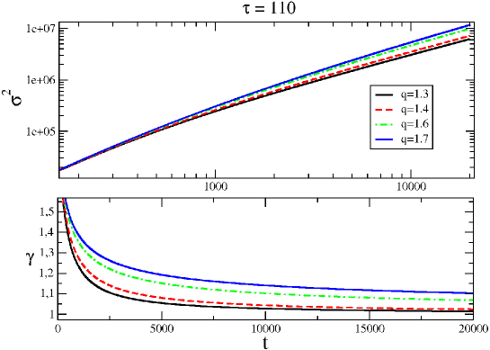
Figure 1: Upper panel: Time evolution of the angular diffusion as predicted by Eq. (15) for different values of $q$. Lower panel: Time evolution of the coefficient $\gamma$, evaluated through the logarithmic derivative .

References

- (1) A. Pluchino, A. Rapisarda, Progress in Theoretical Physics Supplement 162 , 18 (2006); A. Pluchino, V. Latora, A. Rapisarda, Physica A 338, 60 (2004); A. Rapisarda, A. Pluchino, Europhysics News 36, 202 (2005).
- (2) M. Antoni, S. Ruffo, Phys. Rev. E 52, 2361 (1995).
- (3) F. Hohl and M. R. Feix, Astrophys. J. 147, 1164 (1967).
- (4) A. Antoniazzi, D. Fanelli, J. Barré, P.H. Chavanis, T. Dauxois, S. Ruffo, Phys. Rev. E 75, 011112 (2007).
- (5) C. Tsallis, J. Stat. Phys. 52, 479 (1988).
- (6) V. Latora, A. Rapisarda, S. Ruffo, Phys. Rev. Lett. 83, 2104 (1999).
- (7) Y. Y. Yamaguchi, Phys. Rev. E 68, 066210 (2003).
- (8) F. Bouchet, T. Dauxois, Phys. Rev. E 72, 045103(R) (2005).
- (9) C. Tsallis, D.J. Bukman, Phys. Rev. E 54, R2197 (1996).
- (10) L. G. Moyano, C. Anteneodo, Phys. Rev. E 74, 021118 (2006).
- (11) Y.Y. Yamaguchi, F. Bouchet, T. Dauxois, J. Stat. Mechanics: Theory and Experiments P01020 (2007)