Effective elastic theory of smectic-A and smectic-C liquid crystals

Abstract

We analytically derive the effective layer elastic energy of smectic-A and smectic-C liquid crystals by adiabatic elimination of the orientational degree of freedom from the generalized Chen-Lubensky model. In the smectic-A phase, the effective layer bending elastic modulus is calculated as a function of the wavelength of the layer undulation mode. It turns out that an unlocking of the layer normal and the director reduces the layer bending rigidity for wavelengths smaller than the director penetration length. In the achiral smectic-C phase, an anisotropic bending elasticity appears due to the coupling between the layer displacement and director. The effective layer bending rigidity is calculated as a function of the angle $\vartheta$ between the layer undulation wave-vector and the director field. We compute the free energy minimizer $\vartheta=\theta$. It turns out that $\theta$ varies from $0^{\circ}$ to $90^{\circ}$ depending on the tilt angle, undulation wave-length and other elastic constants. We also discover a new important characteristic length and the discontinuous change of $\theta$. Using the elastic constants of Chen-Lubensky model, we determine the parameters of the more macroscopic model [Y. Hatwalne and T. C. Lubensky, Phys. Rev. E 52, 6240 (1995)]. We then discuss the hydrodynamics, and demonstrate the alignment of director and the propagation of the anisotropic layer displacement wave in the presence of an oscillatory wall and a vibrating cylindrical source respectively.

I INTRODUCTION

Liquid crystals have many fascinating physical properties, because they have both the molecular position and the molecular orientation as degrees of freedom de Gennes and Prost (1994). This multiplicity gives rise to interesting phase transition phenomena, including the tricritical and the Lifshitz point in the phase diagram  Chainkin and Lubensky (1995), where the first and second order transitions are switched Keyes et al. (1973); Aharony et al. (1986), and three phases (i.e., the nematic, smectic-A (Sm-A) and smectic-C (Sm-C)) coexist Shashidhar et al. (1984); Drossinos and Ronis (1986), respectively. To explain the phase behavior around the nematic-Sm-A-Sm-C (NAC) Lifshitz point theoretically, a variety of models have been developed de Gennes (1973); Chu and McMillan (1977); Chen and Lubensky (1976); Benguigui (1979); Huang and Lien (1981); Grinstein and Toner (1983). De Gennes de Gennes (1973) and Chu and McMillan Chu and McMillan (1977) introduced a tilt angle and an in-plane director as new degrees of freedom, respectively. Chen and Lubensky Chen and Lubensky (1976) took fourth order derivative of the density field into account. Benguigui Benguigui (1979) and Huang and Lien Huang and Lien (1981) adopted a smectic-C scalar order parameter together with a smectic-A order parameter. Grinstein and Toner Grinstein and Toner (1983) also used the two-dimensional in-plane director component to describe the free energy. Among them, the Chen-Lubensky model is supported by quite a few X-ray scattering experiments  Witanachchi et al. (1983); Safinya et al. (1983); Martinez-Miranda et al. (1986).

In the smectic phase, the layer order and the director often cause a frustration. In chiral liquid crystals, geometrical incompatibility of a uniform smectic order and a helical director configuration leads to a rich variety of defect phases Kitzerow and Bahr (2002). They can be discussed with the Landau-de Gennes model, utilizing an analogy with superconductors in the magnetic field, where the smectic order parameter, the director vector and the chirality are identified with the wave function of a superconducting particle, the electromagnetic vector potential and the external magnetic field, respectively de Gennes (1972). The twist-grain-boundary (TGB) phase is the simplest defect phase where the groups of planes, containing parallel screw dislocations, are regularly stacked with the dislocations in adjacent planes tilted each other at a constant angle, and finite length smectic slabs are inserted between the dislocation planes Renn and Lubensky (1988); Goodby et al. (1989). The Chen-Lubensky model, a higher order extension of the Landau-de Gennes model, is again successful in explaining the structure and phase transition of the TGB${}_{\text{A}}$ and TGB${}_{\text{C}}$ phases, which have the Sm-A and Sm-C slabs respectively Lubensky and Renn (1990); Ismaili et al. (2000). More complex defect structures such as cholesteric and smectic blue phases have been discovered Kitzerow and Bahr (2002). The cubic smectic blue phase (Sm-BP${}_{\text{I}}$) is comprised of a three-dimensional cubic disclination lattice, whose lattice constant is in the order of the wavelength of the visible light Grelet et al. (2001a); DiDonna and Kamien (2002). The isotropic smectic blue phase (Sm-BP${}_{\text{Iso}}$) has fluid-like rheological properties and the detailed structure is completely unknown Yamamoto et al. (2005). Such novel defect structures in principle, should be understood with the Landau-de Gennes and Chen-Lubensky models presented above. However, in fact, these phenomenological models are not appropriate for theoretical explanations of these phases, because of the highly complex spatial structure together with the quite intricate free energy model. DiDonna and Kamien make use of a simpler phenomenological model to discuss the stability of the cubic blue phase DiDonna and Kamien (2002). In their Landau-Peierls form, the director is assumed to be parallel to the layer normal. However, a tilt of the director from the layer normal is reported to weaken the layer bending elasticity in the numerical simulation of the TGB${}_{\text{A}}$ phase Ogawa and Uchida (2006), and to change the structural symmetry of the smectic blue phases in the experimental study Grelet et al. (2001b). Such anomalous properties in the TGB and the smectic blue phases have their origin in a nontrivial elastic mechanism of the undulated smectic layer, combined with the director degree of freedom. Therefore, a modification of the Landau-Peierls model, accommodating the director elasticity of Sm-A and Sm-C phases, would help the understanding of the complex layered structures. In addition, the Landau-Peierls model has the same layer compression and bending elastic energy forms as those of the other layered materials such as block copolymers and surfactant system Ohta and Kawasaki (1986); Gompper and Klein (1992). Thus, the characteristic features of liquid crystals are not very apparent in the original Landau-Peierls model. The director in liquid crystals should affect the layer elasticity, while block copolymers do not possess an orientational degree of freedom especially in the weak segregation limit Leibler (1980). Thus it is worthwhile to derive an intermediately simple model directly from the Chen-Lubensky free energy, eliminating the variation of the director degree of freedom, to clarify the role of the director elasticity in smectic liquid crystals. At the same time, by doing so, we can obtain the phenomenological elastic constants of the macroscopic models DiDonna and Kamien (2002); Hatwalne and Lybensky (1995), in terms of the more microscopic parameters of Chen-Lubensky model.

Dynamics of Sm-C layers is also an interesting topic of liquid crystals de Gennes and Prost (1994); Martin et al. (1972); Buka and Kramer (1996); Pargellis et al. (1992); Carlsson et al. (1995). The director component parallel to layer ($c$-vector) plays an important role on the static and dynamic pattern formation due to the anisotropic elasticity and interaction with flow field Johnson and Saupe (1977); Cladis et al. (1985). Shear flow orients the $c$-vector and results in a novel target pattern with a disclination Cladis et al. (1985); Chevallard et al. (1997). On the other hand, because of the static coupling between the layer displacement and the director, together with the rotational viscosity, an oscillatory wave traveling perpendicularly to the layer normal also rotates and aligns the $c$-vector in a certain direction, even in a uniform oscillatory wave de Gennes and Prost (1994); Clark (1979). It might be useful for an application, for instance, mechanically-active optical devices and sensitive acoustic sensors Clark and Meyer (1973); Clark (1979); Yablonskii et al. (2003); Uto et al. (1997).

This paper is organized as follows. In Section II, we review the original Landau-de Gennes model and derive the effective elastic energy of Sm-A phase. The analysis is extended to Sm-A and Sm-C phases with the generalized Chen-Lubensky model in Section III. Next we conduct a hydrodynamic simulation for Sm-C layer in Section IV. We conclude in Section V.

II Landau-de Gennes model for Smectic-A phase

In this section, we briefly review the Landau-de Gennes model for Sm-A phase, and then calculate the effective layer elastic energy in terms of the layer displacement field. The physical meaning of the results are discussed qualitatively.

Smectic liquid crystals can be described by the density modulation $\Psi(\mbox{\boldmath$r$})$ and the director $\mbox{\boldmath$n$}(\mbox{\boldmath$r$})$. The density field $\Psi(\mbox{\boldmath$r$})$ is a complex order parameter with the absolute value being the amplitude of the smectic order and the phase describing the layer displacement de Gennes (1972). The analogy between liquid crystals and superconductors leads to the phenomenological Landau-de Gennes model for the Sm-A liquid crystals

$$F = F_{\text{layer}}+F_{\text{cpl}}+F_{\text{Frank}},$$ (1a)

$$F_{\text{layer}} = \int d\mbox{\boldmath$r$}\left[\tau|\Psi|^{2}+\frac{g}{2}|\Psi|^{4}\right],$$ (1b)

$$F_{\text{cpl}} = \int d\mbox{\boldmath$r$}\frac{1}{2}\left[B_{\parallel}\left|\left(\mbox{\boldmath$n$}\cdot\nabla-iq_{0}\right)\Psi\right|^{2}+B_{\perp}\left|\mbox{\boldmath$n$}\times\nabla\Psi\right|^{2}\right],$$

$$F_{\text{Frank}} = \int d\mbox{\boldmath$r$}\frac{1}{2}\left[K_{1}(\nabla\cdot{\mbox{\boldmath$n$}})^{2}+K_{2}(\mbox{\boldmath$n$}\cdot\nabla\times{\mbox{\boldmath$n$}})^{2}\right.$$ (1d)

$$\left.+K_{3}(\mbox{\boldmath$n$}\times\nabla\times{\mbox{\boldmath$n$}})^{2}\right].$$

The double-well potential $F_{\text{layer}}$ describes the Nematic-Sm-A (NA) transition. $F_{\text{cpl}}$ and $F_{\text{Frank}}$ are the coupling energy between $\Psi$ and $n$, and the Frank elastic energy. The dimensionless temperature $\tau$ is positive (negative) above (below) the NA point. The constants $B_{\parallel}$ and $B_{\perp}$ are the layer compression elastic coefficients which adjust the layer width to the equilibrium value $d=2\pi/q_{0}$. The Frank elastic constants $K_{i}\,(i=1,2,3)$ correspond to the splay ($i=1$), the twist ($i=2$) and the bend ($i=3$) deformations, respectively.

We consider a perturbation of the uniform Sm-A structure far below the NA point to see the effect of the director tilt from the layer normal. For this purpose, we set $B_{\parallel}=B_{\perp}\equiv B$ and $K_{1}=K_{2}=K_{3}\equiv K$ to simplify the discussion. A more general case is considered in the next section for the Chen-Lubensky model. The amplitude of the smectic order is close to the equilibrium value at low temperature, so we assume

$$\Psi(\mbox{\boldmath$r$})=\Psi_{0}\exp[iq_{0}(z-u(\mbox{\boldmath$r$}))]\,\,\,\left(\Psi_{0}=\sqrt{\frac{\tau}{g}}\right),$$ (2)

where the $z$-axis is set along the equilibrium layer normal, and the layer displacement field $u(\mbox{\boldmath$r$})$ is introduced. The director $n$ can be divided into its spatial average and the deviation:

$$\mbox{\boldmath$n$}(\mbox{\boldmath$r$})=\mbox{\boldmath$e$}_{z}+\delta\mbox{\boldmath$n$}(\mbox{\boldmath$r$}).$$ (3)

The free energy components $F_{\text{cpl}}$ and $F_{\text{Frank}}$ are now simplified as

$$F_{\text{cpl}} = \frac{K}{2\lambda^{2}}\int d\mbox{\boldmath$r$}\left|\nabla u+\delta\mbox{\boldmath$n$}\right|^{2},$$ (4a)

$$F_{\text{Frank}} = \frac{K}{2}\int d\mbox{\boldmath$r$}\left|\nabla\delta\mbox{\boldmath$n$}\right|^{2},$$ (4b)

where $\lambda=\sqrt{K/B}/(\Psi_{0}q_{0})$ is the penetration length Renn and Lubensky (1988), and $\left|\nabla\delta\mbox{\boldmath$n$}\right|^{2}=(\partial_{i}\delta n_{j})(\partial_{i}\delta n_{j})$ (repeated indices are summed up). We next write the linearized effective free energy in terms of $u(\mbox{\boldmath$r$})$. To do this, the director is adiabatically eliminated with the equation,

$$(\b{1}-\mbox{\boldmath$n$}\mbox{\boldmath$n$})\cdot\frac{\delta F}{\delta\mbox{\boldmath$n$}}=0.$$ (5)

The factor $\b{1}-\mbox{\boldmath$n$}\mbox{\boldmath$n$}$ ensures the normalization $\left|\mbox{\boldmath$n$}\right|^{2}=1$, and $\delta n_{z}=0$ because $\left|\mbox{\boldmath$e$}_{z}+\delta\mbox{\boldmath$n$}\right|=1$. Using (4a), (4b) and (5), we obtain the Fourier representations

$$\delta n_{j}(\mbox{\boldmath$q$}) = -\tilde{\kappa}(q)iq_{j}u(\mbox{\boldmath$q$}).$$ (6)

$$\biggl{(}\tilde{\kappa}(q) \equiv \frac{1}{1+\lambda^{2}q^{2}},\,\,\,j=1,2\biggr{)}.$$

Thus the effective free energy is

$$F_{\text{eff}} = \frac{K}{2}\int_{\mbox{\boldmath$q$}}\left[\left(\frac{q_{z}}{\lambda}\right)^{2}+\tilde{\kappa}(q)q_{\perp}^{4}+\tilde{\kappa}(q)q_{\perp}^{2}q_{z}^{2}\right]\left|u(\mbox{\boldmath$q$})\right|^{2},$$ (7)

where we define the $z$-axis and in-plane (x- and y-) axes as the parallel and perpendicular direction respectively (Fig.1). Equation (7) is identical with the Landau-Peierls free energy except for the Lorentzian dependence of the dimensionless layer bending elastic coefficient $\tilde{\kappa}(q)$, and the higher order cross term Chainkin and Lubensky (1995); Clark and Meyer (1973).

The $q$-dependence of $\tilde{\kappa}(q)$ is interpreted qualitatively as follows. We consider a pure undulation case with a constant layer thickness $q_{\parallel}=0$. This condition is, in fact, a sufficiently good approximation to describe experiments in the thermodynamic limit Clark and Meyer (1973). Thus $\mbox{\boldmath$q$}\parallel\delta\mbox{\boldmath$n$}$ is satisfied, which means that only the splay part $\left|\mbox{\boldmath$q$}\cdot\delta\mbox{\boldmath$n$}\right|^{2}$ is nonzero in the three Frank elastic contributions. Since the Landau-de Gennes model (1a) has no layer bending term in the $\Psi$-dependent part, the effective elasticity comes solely from the splay term. In fact, if the director $n$ coincides with the layer normal $m$, the splay term is turned into the layer bending elastic energy:

$$\frac{K}{2}\int d\mbox{\boldmath$r$}\left(\nabla\cdot\mbox{\boldmath$n$}\right)^{2}=2K\int d\mbox{\boldmath$r$}H^{2}.$$ (8)

Here we denote the mean curvature of the smectic layer by $H$.

		(a) $q_{\perp}\ll\lambda^{-1}$		(b) $q_{\perp}\gtrsim\lambda^{-1}$

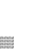
Figure 1: Schematic representation of the undulated layer structure of Sm-A phase. The director and layer normal are (a) almost parallel for $q_{\perp}\ll\lambda^{-1}$ and (b) decoupled for $q_{\perp}\gtrsim\lambda^{-1}$.

Equation (8) is achieved well for $q_{\perp}^{-1}\gg\lambda$, where the director is locked to the layer normal (Fig.1(a)). Oppositely, for $q_{\perp}^{-1}\lesssim\lambda$, the director cannot follow the layer deformation, and the splay term less contributes to the layer elasticity (Fig.1(b)). We note that $\tilde{\kappa}(q)$ can be written also as a function of the root mean squared (RMS) tilt angle $\bar{\alpha}=\sqrt{\left\langle\alpha^{2}\right\rangle}$. With a smooth undulation $u(\mbox{\boldmath$r$})=u_{0}\cos\left(\mbox{\boldmath$q$}_{\perp}\cdot\mbox{\boldmath$r$}\right)\,\,(q_{\perp}\ll\lambda^{-1})$,

$$\tilde{\kappa}(\bar{\alpha})=\frac{1}{1+\left(\sqrt{2}\bar{\alpha}\lambda/u_{0}\right)^{2/3}}.$$ (9)

The detailed derivation is given in Appendix A. The effective layer bending rigidity decays with $\bar{\alpha}$. It implies that the coupling between $m$ and $n$ is certainly essential.

In fact, for any $\Psi$, the locking term is found in the coupling term (LABEL:eq:L-deGcpl)

$$F_{cpl}=\frac{1}{2}\int d\mbox{\boldmath$r$}\left[B_{\parallel}\biggl{|}\mbox{\boldmath$n$}\cdot\biggl{(}-i\nabla{\Psi_{0}}+\Psi_{0}\mbox{\boldmath$n$}(|\nabla{\phi}|-q_{0})+\Psi_{0}|\nabla{\phi}|(\mbox{\boldmath$m$}-\mbox{\boldmath$n$})\biggr{)}\biggr{|}^{2}\right.$$

$$\left.+B_{\perp}\biggl{|}\mbox{\boldmath$n$}\times\biggl{(}-i\nabla{\Psi_{0}}+\Psi_{0}|\nabla{\phi}|\mbox{\boldmath$m$}\biggr{)}\biggr{|}^{2}\right]$$

(10)

where the complex order parameter is decomposed into the amplitude and the phase: $\Psi(\mbox{\boldmath$r$})=\Psi_{0}(\mbox{\boldmath$r$})\exp(i\phi(\mbox{\boldmath$r$}))$, and the gradient of the phase component defines the layer normal vector $\mbox{\boldmath$m$}(\mbox{\boldmath$r$})=\nabla{\phi}/|\nabla{\phi}|$. In the parallel part, the first term favors a uniform smectic modulation amplitude, the second is the layer compression energy and the last term locks the director along the layer normal. In the perpendicular part, on the other hand, the first term is again the amplitude homogenizing contribution, and the second term reduces the director component perpendicular to the layer normal ($c$-vector) as long as the coefficient $B_{\perp}$ is positive. The Sm-C phase is stable with a negative $B_{\perp}$, as we shall see in the next section.

III Generalized Chen-Lubensky model for smectic-A and -C phases

In this section, we introduce the Chen-Lubensky model in the generalized way. Then the effective elastic energy is calculated for both Sm-A and Sm-C phases. After a physical interpretation of the Sm-A energy, the effective layer bending elasticity of the Sm-C phase is discussed. The anisotropy is characterized by the angle $\vartheta$ between the $c$-vector and the layer bending direction. The state diagrams for the easiest bending angle $\theta$ are studied. The free energy as a function of $\vartheta$ is also calculated. Finally, the model parameters of the more macroscopic free energy Hatwalne and Lybensky (1995) are determined with those of Chen-Lubensky model.

III.1 Generalized Chen-Lubensky model

By adding higher order gradient terms, one can extend the Landau-de Gennes free energy to reproduce the achiral Sm-C phase. The Chen-Lubensky model is given in the most generalized form:

$$F = \frac{K_{3}}{2}\tilde{F}\,\,\,\,\,\,\,$$

$$\left(\tilde{F}\right. = \left.\tilde{F}_{\text{layer}}+\tilde{F}_{\text{cpl}}^{(2)}+\tilde{F}_{\text{cpl}}^{(4)}+\tilde{F}_{Frank}\right),$$ (11a)

$$\Psi_{0}^{2}q_{0}^{2}\tilde{F}_{\text{layer}} = 2\int d\mbox{\boldmath$r$}\left[\tilde{\tau}|\Psi|^{2}+\frac{\tilde{g}}{2}|\Psi|^{4}\right],$$ (11b)

$$\Psi_{0}^{2}q_{0}^{2}\tilde{F}_{\text{cpl}}^{(2)} = 2\int d\mbox{\boldmath$r$}\left[\left(\tilde{C}_{\parallel}n_{i}n_{j}+\tilde{C}_{\perp}\delta_{ij}^{\perp}\right)(D_{i}\Psi)(D_{j}\Psi)^{*}\right],$$

$$\Psi_{0}^{2}q_{0}^{2}\tilde{F}_{\text{cpl}}^{(4)} = 2\int d\mbox{\boldmath$r$}\left[\tilde{D}_{\parallel}\left|n_{i}n_{j}D_{i}D_{j}\Psi\right|^{2}\right.$$ (11c)

$$+\tilde{D}_{\parallel\perp}\left((n_{i}n_{j}D_{i}D_{j}\Psi)\left(\delta_{kl}^{\perp}D_{k}D_{l}\Psi\right)^{*}+c.c.\right)$$

$$\left.+\tilde{D}_{\perp}\left|\delta_{ij}^{\perp}D_{i}D_{j}\Psi\right|^{2}\right],$$

$$\tilde{F}_{\text{Frank}} = \int d\mbox{\boldmath$r$}\left[\left(1+\tilde{\kappa}_{1}\right)(\nabla\cdot{\mbox{\boldmath$n$}})^{2}\right.$$

$$+\left(1+\tilde{\kappa}_{2}\right)K_{2}(\mbox{\boldmath$n$}\cdot\nabla\times{\mbox{\boldmath$n$}})^{2}$$

$$\left.+\left\{\mbox{\boldmath$n$}\times\left(\nabla\times{\mbox{\boldmath$n$}}\right)\right\}^{2}\right],$$

where $D_{i}=\partial_{i}-iq_{0}n_{i}$ is the covariant derivative and $\delta_{ij}^{\perp}=\delta_{ij}-n_{i}n_{j}$ is the projection operator. The elastic constants are $\tilde{C}_{\parallel}$ and $\tilde{C}_{\perp}$ for the second order gradient term $\tilde{F}_{\text{cpl}}^{(2)}$, $\tilde{D}_{\parallel}$, $\tilde{D}_{\parallel\perp}$ and $\tilde{D}_{\perp}$ for the fourth order terms $\tilde{F}_{\text{cpl}}^{(4)}$.

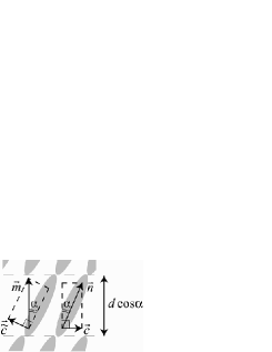
Figure 2: Schematic representation of the $c$ and $\tilde{\mbox{\boldmath$c$}}$ vector defined by the layer normal vector $m$ and the director $n$. It is obvious that $\tilde{\mbox{\boldmath$c$}}\rightarrow-\mbox{\boldmath$c$}$ in the small tilt limit $\alpha\rightarrow 0$.

The physical meaning of the covariant derivative is as follows (Fig.2). With the sinusoidal density profile $\Psi(\mbox{\boldmath$r$})=\Psi_{0}\exp\left(i\phi(\mbox{\boldmath$r$})\right)$ and the layer normal vector $\mbox{\boldmath$m$}\equiv\nabla\phi/|\nabla\phi|$, one obtains $\mbox{\boldmath$D$}\Psi=i|\nabla\phi|(\mbox{\boldmath$m$}-\mbox{\boldmath$n$}\cos\alpha)\Psi\equiv i\tilde{\mbox{\boldmath$c$}}|\nabla\phi|\Psi$, where $\alpha$ is the angle between $n$ and $m$, and $\tilde{\mbox{\boldmath$c$}}$ is the layer normal vector component perpendicular to the molecular orientation, which coincides with $-\mbox{\boldmath$c$}$ for $\alpha\rightarrow 0$. Because $\tilde{C}_{\parallel}|\mbox{\boldmath$n$}\cdot\mbox{\boldmath$D$}\Psi|^{2}=0$ and $\tilde{C}_{\perp}|\mbox{\boldmath$n$}\times\mbox{\boldmath$D$}\Psi|^{2}=\tilde{C}_{\perp}\Psi_{0}^{2}|\nabla\phi|^{2}\tilde{\mbox{\boldmath$c$}}^{2}$, Sm-C phase is equilibrated with a combination of a negative $\tilde{C}_{\perp}$ and stabilizing fourth-order covariant derivatives.

The scattering function is readily calculated as

$$S(\mbox{\boldmath$q$})=\frac{S_{0}\tilde{\tau}_{0}}{\tilde{\tau}_{0}+\tilde{D}_{\parallel}(q_{\parallel}-q_{0})^{4}+(\tilde{C}_{\parallel}+2\tilde{D}_{\parallel\perp}q_{\perp}^{2})(q_{\parallel}-q_{0})^{2}+\tilde{D}_{\perp}(q_{\perp}^{2}-q_{0\perp}^{2})^{2}},$$ (12)

where we set $\tilde{\tau}_{0}=\tilde{\tau}-\tilde{C}_{\perp}^{2}/(4\tilde{D}_{\perp})$ and $q_{0\perp}^{2}=-\tilde{C}_{\perp}/(2\tilde{D}_{\perp})$. The relations of the present generalized model to the other models are shown in Table 1. One can obtain the original Chen-Lubensky model if $\tilde{D}_{\parallel}=\tilde{D}_{\parallel\perp}=0$ and $\tilde{D}_{\perp}\neq 0$. With $\tilde{C}_{\parallel}=B_{\parallel}/(2\Psi_{0}^{2}q_{0}^{2})$, $\tilde{C}_{\perp}=B_{\perp}/(2\Psi_{0}^{2}q_{0}^{2})$ and $\tilde{D}_{\parallel}=\tilde{D}_{\parallel\perp}=\tilde{D}_{\perp}=0$, the Chen-Lubensky model is reduced to the Landau-de Gennes model (1a).

model type	parameter list
original Chen-Lubensky model Chen and Lubensky (1976)	$\tilde{D}_{\parallel}=\tilde{D}_{\parallel\perp}=0$, $\tilde{D}_{\perp}\neq 0$
model of Luk’yanchuk (1998)	$\tilde{D}_{\parallel}=\tilde{D}_{\parallel\perp}=\tilde{D}_{\perp}\neq 0$
model of Kundagrami and Lubensky (2003) (in the vicinity of $q_{\parallel}=q_{0}$)	$\tilde{C}_{\parallel}=4\tilde{D}_{\parallel}q_{0}^{2}\neq 0$, $\tilde{D}_{\parallel\perp},\tilde{D}_{\perp}\neq 0$
Landau-de Gennes model (1a)	$\tilde{C}_{i}=B_{i}/(2\Psi_{0}^{2}q_{0}^{2})\,\,\,(i=\parallel,\perp)$, $\tilde{D}_{\parallel}=\tilde{D}_{\parallel\perp}=\tilde{D}_{\perp}=0$

Table 1: Relationships between the generalized Chen-Lubensky and other models with the corresponding parameter lists.

The equilibrium director in the Sm-C phase tilts against the layer normal at the angle,

$$\alpha=\tan^{-1}\left(\frac{1}{q_{0}}\sqrt{\frac{-\tilde{C}_{\perp}}{2\tilde{D}_{\perp}}}\right).$$ (13)

Next we consider a perturbation of the uniform equilibrium configuration with the generalized Chen-Lubensky model. The director perturbation is given by

$$\delta\mbox{\boldmath$n$}(\mbox{\boldmath$r$})=\mbox{\boldmath$n$}(\mbox{\boldmath$r$})-\mbox{\boldmath$N$},$$ (14)

where $N$ is the equilibrium director and equals $\left(\sin\alpha\cos\psi,\sin\alpha\sin\psi,\cos\alpha\right)$. The azimuthal angle $\psi$ is the Goldstone mode in the Sm-C phase. The layer deformation is expressed only by $u(\mbox{\boldmath$r$})$

$$\Psi(\mbox{\boldmath$r$})=\Psi_{0}\exp\left[\frac{iq_{0}}{N_{3}}\left(z-u(\mbox{\boldmath$r$})\right)\right].$$ (15)

The equilibrium condition (5), equivalent to $\mbox{\boldmath$n$}\parallel\delta\tilde{F}/\delta\mbox{\boldmath$n$}$, reads

$$\frac{\delta\tilde{F}}{\delta n_{i}}-\frac{N_{i}+\delta n_{i}}{N_{3}+\delta n_{3}}\frac{\delta\tilde{F}}{\delta n_{3}} = 0\,\,\,(i=1,2).$$ (16a)

The perturbation expansion requires

$$\gamma_{i}\frac{\delta\tilde{F}}{\delta n_{3}}^{(0)}=\frac{\delta\tilde{F}}{\delta n_{i}}^{(1)}-\gamma_{i}\frac{\delta\tilde{F}}{\delta n_{3}}^{(1)}-\frac{\delta n_{i}}{N_{3}}\frac{\delta\tilde{F}}{\delta n_{3}}^{(0)}=0\,\,\,\,(i=1,2),$$ (17)

where $\gamma_{i}=N_{i}/N_{3}\,(i=1,2)$, and $O^{(n)}$ means the $n$th order perturbative part of $O$ in terms of $\delta\mbox{\boldmath$n$}$ and $u$. Equation (17) has two possible solutions. We obtain the Sm-A phase ($\mbox{\boldmath$N$}=\mbox{\boldmath$e$}_{3}$) if $\left(\delta\tilde{F}/\delta n_{3}\right)^{(0)}\neq 0$, otherwise the Sm-C phase with the director tilt angle $\alpha$ (13).

III.2 Effective Sm-A free energy

The Sm-A case is quite simple: $\gamma_{1}=\gamma_{2}=0$ and $N_{3}=1$. Following the same procedure as in Sec. II, the effective free energy is calculated as

$$\delta n_{i}(\mbox{\boldmath$q$}) = -\frac{2i(\tilde{C}_{\perp}+\tilde{D}_{\parallel}q_{\parallel}^{2}+\tilde{D}_{\perp}q_{\perp}^{2})}{2\tilde{C}_{\perp}+\tilde{D}^{{}^{\prime}}q_{\perp}^{2}+q^{2}}q_{i}u(\mbox{\boldmath$q$})\,\,\,\,(i=1,2),\,\,\,\,\,\,\,\,\,\,\,\delta n_{3}(\mbox{\boldmath$r$})=0,$$ (18)

$$\tilde{F} = 2\int_{\mbox{\boldmath$q$}}\biggl{[}\tilde{C}_{\parallel}q_{\parallel}^{2}+\tilde{D}_{\parallel}q_{\parallel}^{4}+2\tilde{D}_{\parallel\perp}q_{\parallel}^{2}q_{\perp}+\tilde{D}_{\perp}q_{\perp}^{4}\biggr{.}$$

$$\biggl{.}+\frac{\tilde{C}_{\perp}q_{\perp}^{2}\left(\tilde{D}^{{}^{\prime}}q_{\perp}^{2}+q^{2}\right)-2q_{\perp}^{2}\left(\tilde{D}_{\parallel}q_{\parallel}^{2}+\tilde{D}_{\perp}q_{\perp}^{2}\right)\left(2\tilde{C}_{\perp}+\tilde{D}_{\parallel}q_{\parallel}^{2}+\tilde{D}_{\perp}q_{\perp}^{2}\right)}{2\tilde{C}_{\perp}+\tilde{D}^{{}^{\prime}}q_{\perp}^{2}+q^{2}}\biggr{]}|u(\mbox{\boldmath$q$})|^{2},$$

where $\int_{\mbox{\boldmath$q$}}[\cdots]\equiv\int d\mbox{\boldmath$q$}[\cdots]/(2\pi)^{3}$ and $\tilde{D}^{{}^{\prime}}\equiv 2\tilde{D}_{\perp}+\tilde{\kappa}_{1}$. The twist and bend contributions of Frank energy do not appear in the effective free energy because $\delta\mbox{\boldmath$n$}_{\perp}\parallel\mbox{\boldmath$q$}_{\perp}$. The layer compression term has no director contribution, because the layer width strain energy should be the quadratic form $\partial_{z}u+\delta n_{z}$, and the higher order term $\delta n_{z}$ is neglected.

Next we compare the previous Landau-de Gennes and the present Chen-Lubensky model briefly, to understand the role of the fourth order gradient terms. By setting $\tilde{D}_{\parallel}=\tilde{D}_{\parallel\perp}=\tilde{\kappa}_{1}=0$, Eq.(III.2) is reduced to the simpler form

$$\tilde{F} = 2\int_{\mbox{\boldmath$q$}}\left[\tilde{C}_{\parallel}q_{\parallel}^{2}+\tilde{\kappa}(\mbox{\boldmath$q$})q_{\perp}^{4}+\frac{\tilde{C}_{\perp}+\tilde{D}_{\perp}q_{\perp}^{2}}{2\tilde{C}_{\perp}+2\tilde{D}_{\perp}q_{\perp}^{2}+q^{2}}q_{\parallel}^{2}q_{\perp}^{2}\right]|u(\mbox{\boldmath$q$})|^{2},$$ (20)

$$\left(\tilde{\kappa}(\mbox{\boldmath$q$})=\frac{\tilde{C}_{\perp}+2\tilde{D}_{\perp}\tilde{C}+\tilde{D}_{\perp}q_{\perp}^{2}}{2\tilde{C}_{\perp}+2\tilde{D}_{\perp}q_{\perp}^{2}+q^{2}}\right).$$

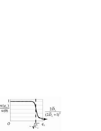
Figure 3: Plot of the effective layer undulation modulus $\tilde{\kappa}(q_{3}=0,\,q_{\perp})$ in (20). The Lorentzian curve with the offset $(\sim\tilde{D}_{\perp})$ decays with the characteristic wave number $\sim\sqrt{\tilde{C}_{\perp}}$. The fourth-order gradient coefficients are typically quite small than the second order coefficients.

This is identical with the effective Landau-de Gennes free energy (7) if $\tilde{D}_{\perp}=0$. The profile of $\tilde{\kappa}(\mbox{\boldmath$q$})$ is depicted in Fig.3. The layer bending modulus only from the density contribution can be considered as $\tilde{\kappa}(q_{\perp}\rightarrow\infty)=2\tilde{D}_{\perp}/(2\tilde{D}_{\perp}+1)$ because the splay vanishes at $q_{\perp}\rightarrow\infty$.

III.3 Effective free energy for Sm-C phase

Next we calculate the effective free energy for the Sm-C phase. Using $\delta\tilde{F}^{(0)}/\delta n_{3}=-4\left\{\tilde{C}_{\perp}+2\tilde{D}_{\perp}q_{0}^{2}\left((1/N_{3}^{2})-1\right)\right\}/N_{3}=0$, the perturbed equation of state is given in the matrix form

$$\mbox{\boldmath$M$}\delta\mbox{\boldmath$n$}_{\perp}(\mbox{\boldmath$q$}) = \mbox{\boldmath$v$}(\mbox{\boldmath$q$}),$$ (21a)

$$M = \left(\begin{array}[]{cc}\tilde{D}^{{}^{\prime}}\tilde{q}_{2}^{2}+\left(1-N_{2}^{2}\right)q^{2}+2N_{1}^{2}A+\tilde{\kappa}_{2}\tilde{q}_{\perp 2}^{2}&-\tilde{D}^{{}^{\prime}}\tilde{q}_{1}\tilde{q}_{2}+N_{1}N_{2}\left(q^{2}+2A\right)-\tilde{\kappa}_{2}\tilde{q}_{\perp 1}\tilde{q}_{\perp 2}\\ -\tilde{D}^{{}^{\prime}}\tilde{q}_{1}\tilde{q}_{2}+N_{1}N_{2}\left(q^{2}+2A\right)-\tilde{\kappa}_{2}\tilde{q}_{\perp 1}\tilde{q}_{\perp 2}&\tilde{D}^{{}^{\prime}}\tilde{q}_{1}^{2}+\left(1-N_{1}^{2}\right)q^{2}+2N_{2}^{2}A+\tilde{\kappa}_{2}\tilde{q}_{\perp 1}^{2}\end{array}\right),$$ (21d)

$$\mbox{\boldmath$v$}(\mbox{\boldmath$q$}) = 2i\left(\begin{array}[]{c}E\gamma_{1}+\tilde{d}\tilde{q}_{2}\\ E\gamma_{2}-\tilde{d}\tilde{q}_{1}\\ \end{array}\right)u(\mbox{\boldmath$q$}),$$ (21h)

where we use the first order terms of the normalization condition $\delta n_{3}=-\gamma_{1}\delta n_{1}-\gamma_{2}\delta n_{2}$. Here we introduced the abbreviations

$$A \equiv \frac{1}{N_{3}^{2}}\left(\tilde{C}_{\parallel}+4\tilde{D}_{\perp}q_{0}^{2}+\frac{2\tilde{D}_{\parallel\perp}q_{0}^{2}N_{\perp}^{2}}{N_{3}^{2}}\right),$$ (22a)

$$E \equiv \frac{4\tilde{D}_{\perp}q_{0}^{2}\tilde{q}_{3}}{N_{3}}-\left(\tilde{C}_{\parallel}+\frac{2\tilde{D}_{\parallel\perp}q_{0}^{2}N_{\perp}^{2}}{N_{3}^{2}}\right)\mbox{\boldmath$N$}\cdot\mbox{\boldmath$q$},$$ (22b)

$$\tilde{\mbox{\boldmath$q$}} \equiv \mbox{\boldmath$q$}\times\mbox{\boldmath$N$},$$ (22c)

$$\tilde{\mbox{\boldmath$q$}}_{\perp} \equiv \mbox{\boldmath$q$}-\mbox{\boldmath$N$}\left(\mbox{\boldmath$N$}\cdot\mbox{\boldmath$q$}\right)=\mbox{\boldmath$N$}\times\tilde{\mbox{\boldmath$q$}},$$ (22d)

$$\tilde{d} \equiv \tilde{D}_{\parallel\perp}\left(\mbox{\boldmath$N$}\cdot\mbox{\boldmath$q$}\right)^{2}+\tilde{D}_{\perp}\left(\mbox{\boldmath$N$}\times\mbox{\boldmath$q$}\right)^{2}.$$ (22e)

The smectic free energy is invariant under a uniform layer displacement, and the solution of the equation of state (21a) for $q=0$ is $\mbox{\boldmath$N$}\cdot\delta\mbox{\boldmath$n$}_{\perp}=\delta n_{3}=0$. This is nothing but a uniform rotational Goldstone mode of the $c$-vector.

Inverting the matrix $M$, we obtain the expression for the director deformation

$$\left(\begin{array}[]{c}\delta n_{1}(\mbox{\boldmath$q$})\\ \delta n_{2}(\mbox{\boldmath$q$})\\ \end{array}\right) = \frac{2iu(\mbox{\boldmath$q$})}{D_{C}}\left(\begin{array}[]{r}-N_{3}\left(E\tilde{D}^{{}^{\prime}}\tilde{q}_{2}+2\tilde{d}AN_{2}\right)\tilde{q}_{3}+EN_{3}N_{1}q^{2}\\ -E\tilde{\kappa}_{2}\tilde{q}_{\perp 1}\tilde{q}_{\perp 3}-N_{3}\tilde{d}\tilde{q}_{\perp 1}\left(q^{2}+\tilde{\kappa}_{2}\tilde{q}^{2}\right)\\ N_{3}\left(E\tilde{D}^{{}^{\prime}}\tilde{q}_{1}+2\tilde{d}AN_{1}\right)\tilde{q}_{3}+EN_{3}N_{2}q^{2}\\ -E\tilde{\kappa}_{2}\tilde{q}_{\perp 2}\tilde{q}_{\perp 3}-N_{3}\tilde{d}\tilde{q}_{\perp 2}\left(q^{2}+\tilde{\kappa}_{2}\tilde{q}^{2}\right)\end{array}\right),$$ (29)

where the determinant of $M$ is given by

$$D_{C} = N_{3}^{2}\left[\left(\tilde{D}^{{}^{\prime}}+\tilde{\kappa}_{2}\right)q^{2}\tilde{q}^{2}+\tilde{D}^{{}^{\prime}}\tilde{\kappa}_{2}\tilde{q}^{4}+2\tilde{D}^{{}^{\prime}}A\tilde{q}_{3}^{2}+2A\tilde{\kappa}_{2}\tilde{q}_{\perp 3}^{2}+2N_{\perp}^{2}q^{2}A+q^{4}\right].$$ (30)

Now in the Sm-C phase, $\delta\mbox{\boldmath$n$}\nparallel\mbox{\boldmath$q$}_{\perp}$ even at the pure undulation ($q_{3}=0$). So not only the splay Frank elastic energy but also the twist and bend terms have contributions to the layer bending elastic energy. The splay term favors the state with $\mbox{\boldmath$q$}\perp\delta\mbox{\boldmath$n$}$ (we call it the $\mbox{\boldmath$q$}\perp\delta\mbox{\boldmath$n$}$ state), and both the twist and the bending terms favor the $\mbox{\boldmath$q$}\parallel\delta\mbox{\boldmath$n$}$ state. In such a layered smectic phase with the spontaneously symmetry breaking layer normal direction and with the rotational Goldstone mode of the $c$-vector, the three Frank elastic terms have anisotropic energy contributions, together with the anisotropic coupling constants. The leading order terms including $\tilde{D}_{\parallel}$, $\tilde{D}_{\perp}$ and $\tilde{D}_{\parallel\perp}$ are $(\nabla^{2}_{\parallel}u)^{2}$, $(\nabla^{2}_{\perp}u+\nabla\cdot{\mbox{\boldmath$n$}})^{2}$ and $(\nabla^{2}_{\parallel}u)(\nabla^{2}_{\perp}u+\nabla\cdot{\mbox{\boldmath$n$}})$, which favor $\mbox{\boldmath$N$}\perp\mbox{\boldmath$q$}$, $\mbox{\boldmath$N$}\parallel\mbox{\boldmath$q$}$ and the intermediate state respectively.

Anisotropy due to the $c$-vector is apparent in the pure undulation case ($q_{3}=0$). Let $\vartheta$ be the angle between $c$ and $\mbox{\boldmath$q$}_{\perp}$. The effective free energy is calculated with (29),

$$\tilde{F} = 2\int_{\mbox{\boldmath$q$}_{\perp}}\tilde{f}=4\int_{\mbox{\boldmath$q$}_{\perp}}q_{\perp}^{4}|u(\mbox{\boldmath$q$})|^{2}\left(\kappa_{u}(x)+\kappa_{n}(\mbox{\boldmath$q$},x)\right),$$ (31a)

$$\kappa_{u}(x) = \frac{\tilde{D}_{\parallel}N_{\perp}^{4}x^{2}+2\tilde{D}_{\parallel\perp}N_{\perp}^{2}xy+\tilde{D}_{\perp}y^{2}}{N_{3}^{2}},$$ (31b)

$$\kappa_{n}(\mbox{\boldmath$q$},x) = \frac{1}{N_{3}^{2}}\frac{\tilde{D}_{n1}(x)N_{3}^{2}q_{\perp}^{2}\lambda_{A}^{2}+\tilde{D}_{n2}(x)N_{\perp}^{2}}{\tilde{D}_{n3}(x)N_{3}^{2}q_{\perp}^{2}\lambda_{A}^{2}+\tilde{D}_{n4}(x)N_{\perp}^{2}},$$ (31c)

$$\tilde{D}_{n1}(x) = -2\left(\tilde{D}_{\parallel\perp}x+\tilde{D}_{\perp}y\right)^{2}y\left(1+\tilde{\kappa}_{2}y\right),$$ (32a)

$$\tilde{D}_{n2}(x) = xN_{3}^{2}\left\{1+\tilde{D}^{{}^{\prime}}y-4\left(\tilde{D}_{\parallel\perp}x+\tilde{D}_{\perp}y\right)\right\}\left(1+\tilde{\kappa}_{2}y\right),$$ (32b)

$$-4\left(\tilde{D}_{\parallel\perp}x+\tilde{D}_{\perp}y\right)^{2}\left(1-x\right),$$

$$\tilde{D}_{n3}(x) = \left(1+\tilde{D}^{{}^{\prime}}y\right)\left(1+\tilde{\kappa}_{2}y\right),$$ (32c)

$$\tilde{D}_{n4}(x) = 2\left(\tilde{D}^{{}^{\prime}}\left(1-x\right)+\tilde{\kappa}_{2}N_{3}^{2}x+1\right),$$ (32d)

where $x\equiv\cos^{2}\vartheta$ and $y(x)=1-N_{\perp}^{2}x$. The effective layer bending elasticity contains the two components: $\kappa_{u}(x)$ is the density contribution without the director deformation, and $\kappa_{n}(q_{\perp},x)$ comes both from the density and director elasticity. The director part has a new characteristic length-scale $\lambda_{A}\equiv 1/\sqrt{A}$, determined by the ratio of the Frank elasticity and the combination of the second and fourth order density gradient terms (22a). Taking the Landau-de Gennes limit $\tilde{D}_{i}\rightarrow 0\,\,(i=\perp,\parallel\perp,\parallel)$ and $\alpha\rightarrow 0$, $\lambda_{A}$ is reduced to the parallel penetration length $\lambda_{\parallel}=\sqrt{\tilde{C}_{\parallel}}$. It is completely different from the Sm-A case where the characteristic length is $\lambda_{\perp}=\sqrt{\tilde{C}_{\perp}}$ (20).

We will compare this result with the previous works in Sec. III E.

III.4 State diagram for Sm-C phase

In the following, we examine the minimizer $\vartheta=\theta$ for $\tilde{F}(\vartheta)$ (31a). The angles $\vartheta$ and $\theta$ are spatially uniform by assumption.

We first consider the one Frank constant case: $K_{1}=K_{2}=K_{3}$. In this case, the calculation and evaluation of the free energy become quite simple with no further approximation. One can show that the free energy density $\tilde{f}(x)$ is a convex function throughout $0\leq x\leq 1$, because a stability of the smectic layer requires the inequality $\det(\tilde{D})\equiv\tilde{D}_{\parallel}\tilde{D}_{\perp}-\tilde{D}_{\parallel\perp}^{2}>0$ (see Appendix B). Thus the behavior of the free energy minimum is determined only by $\tilde{f}^{{}^{\prime}}(0)$, $\tilde{f}^{{}^{\prime}}(1)$ and $\det(\tilde{D})$. There are three possible cases for the first derivative $\tilde{f}^{{}^{\prime}}(x)$:
(i) $\tilde{f}^{{}^{\prime}}(0)>0$ (so $\tilde{f}^{{}^{\prime}}(1)>0)$
  The minimum of the free energy is at $\theta=90^{\circ}$
(ii) $\tilde{f}^{{}^{\prime}}(0)<0$ and $\tilde{f}^{{}^{\prime}}(1)>0$
  The favored angle $\theta$ exists between $0^{\circ}$ and $90^{\circ}$.
(iii) $\tilde{f}^{{}^{\prime}}(0)<0$ and $\tilde{f}^{{}^{\prime}}(1)<0$.
  The free energy minimum is at $\theta=0^{\circ}$, and the director tends to be aligned to the layer bending direction.

(a) $\alpha=10^{\circ},q_{\perp}=2\times 10^{6}$cm-1		(b) $\alpha=10^{\circ},q_{\perp}=2\times 10^{7}$cm-1
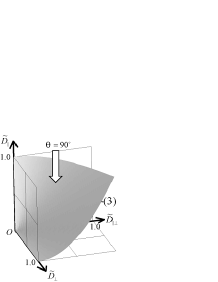
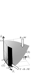
(c) $\alpha=30^{\circ},q_{\perp}=2\times 10^{6}$cm-1		(d) $\alpha=50^{\circ},q_{\perp}=2\times 10^{6}$cm-1

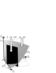
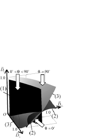
Figure 4: State diagrams with $\tilde{D}_{\perp}$, $\tilde{D}_{\parallel\perp}$ and $\tilde{D}_{\parallel}$ in the one Frank constant approximation. We use $q_{0}=2\times 10^{7}$cm^-2 and $\tilde{C}_{\parallel}=4\times 10^{12}$cm${}^{-1}\left(\sim\lambda_{\parallel}^{-2}\right)$ as a set of typical values Renn and Lubensky (1988); Navailles et al. (1995). The planes $\tilde{f}^{{}^{\prime}}(0)=0$, $\tilde{f}^{{}^{\prime}}(1)=0$ and $\det(\tilde{D})=\tilde{D}_{\perp}\tilde{D}_{\parallel}-\tilde{D}_{\parallel\perp}^{2}=0$ are denoted by the plane (1), (2) and (3) respectively.

The fixed parameters are set to be typical values and used in followings if not specified: $q_{\perp}=2\times 10^{7}$cm^-1 and $\tilde{C}_{\parallel}=\lambda^{-2}_{\parallel}=4\times 10^{12}$cm^-2 Renn and Lubensky (1988); Navailles et al. (1995). We limit the possible parameter range of $\left\{\tilde{D}_{i}\,|\,i=\parallel,\parallel\perp,\perp\right\}$ to $0<\tilde{D}_{i}<1$, because of the stability of the free energy, the relation $\tilde{D}_{\perp}\sim d^{2}/(\lambda_{\perp}N_{\perp})^{2}$ holds, and the feasibility of the Landau-de Gennes model $(\tilde{D}_{i}=0)$ in the Sm-A phase. In fact, one of the scattering experiments shows that $\tilde{D}_{\parallel\perp}$, $\tilde{D}_{\parallel}\simeq 0$ and $\tilde{D}_{\perp}(\sim 10^{-4})\ll 1$ Martinez-Miranda et al. (1986), where only the trivial $\theta=90^{\circ}$ state is expected to be observed as the previous work implies Hatwalne and Lybensky (1995); Johnson and Saupe (1977). However, depending on the material, one might be able to obtain a wide range of the parameter sets within $0<\tilde{D}_{i}\lesssim 1$. The three-dimensional state diagrams for $\tilde{D}_{\parallel}$, $\tilde{D}_{\parallel\perp}$ and $\tilde{D}_{\perp}$ are given in Fig.4. State boundaries are determined by the conditions (1) $\tilde{f}^{{}^{\prime}}(0)=0$, (2) $\tilde{f}^{{}^{\prime}}(1)=0$, and (3) $\det(\tilde{D})=0$.

We again note that the smectic layer elasticity consists only of the density and the Frank elastic energies and the coupling energy between the layer normal and the director. All the following results will be explained in terms of combinations of the three elastic contributions.

The $\theta=90^{\circ}$ state dominates for small $\alpha$ and $q_{\perp}<\lambda_{A}^{-1}(\sim 10^{7}$cm${}^{-1})$ (Fig.4(a)). When $q_{\perp}\gtrsim\lambda_{A}^{-1}$, on the other hand, the Frank elasticity less contributes to $\tilde{\kappa}(\mbox{\boldmath$q$})$, and anisotropic density terms dominate (Fig.4(b)), being enhanced for larger $\alpha$ (Fig.4(c)). Thus various angle $\theta$ can appear. In experiment, the largest tilt angle $\alpha$ that has been reported to our knowledge is $37^{\circ}$ Meiboom and Hewitt (1975). So the possible stable $\theta$ state might be limited to $0^{\circ}<\theta\leq 90^{\circ}$, as we see from the diagrams for $\alpha\leq 40^{\circ}$. Nevertheless, if the $\alpha=50^{\circ}$ molecular tilt is achieved, there exists the stable $\theta=0^{\circ}$ state (Fig.4(d)).

In each state diagram, the behavior of $\theta$ is quite sensitive to $\tilde{D}_{\perp}$ compared with $\tilde{D}_{\parallel\perp}$ and $\tilde{D}_{\parallel}$. This is because the elasticity of the vector $\tilde{\mbox{\boldmath$c$}}$ $\left(\simeq-\mbox{\boldmath$c$}\right)$ is dominated by the elastic terms including $\tilde{D}_{\perp}$, as we discussed in Sec.II A. The ratio between $\tilde{C}_{\perp}$ and $\tilde{D}_{\perp}$ is uniquely determined by the tilt angle $\alpha$ (13), so the value of $\tilde{D}_{\perp}$ controls the preference of $\mbox{\boldmath$q$}_{\perp}\parallel\mbox{\boldmath$N$}$. Thus the stable state changes from $\theta=90^{\circ}$ to $0^{\circ}<\theta<90^{\circ}$ and $\theta=0^{\circ}$ as $\tilde{D}_{\perp}$ grows. On the other hand in Fig.4(d), the $\theta=0^{\circ}$ state transits to the $0^{\circ}<\theta<90^{\circ}$ state with the increment of $\tilde{D}_{\parallel}$.

		(a) $\alpha=40^{\circ}$		(b) $\alpha=50^{\circ}$		(c) $\alpha=50^{\circ}$, $\tilde{D}_{\perp}=0.2$

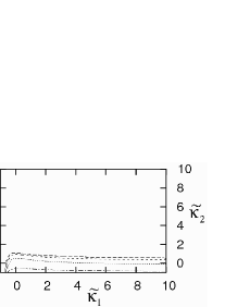
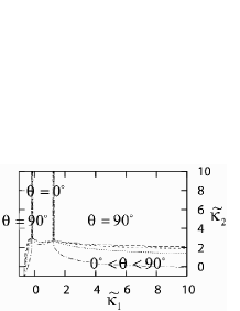
Figure 5: State diagrams in terms of $\tilde{\kappa}_{1}$ and $\tilde{\kappa}_{2}$ with different tilt angles. (a) The $0^{\circ}<\theta<90^{\circ}$ domain gradually disappears as $\alpha\rightarrow 0$. For $\alpha=40^{\circ}$, the $0^{\circ}<\theta<90^{\circ}$ domain grows around $\tilde{\kappa}_{1}\simeq 0$. (b) For $\alpha=50^{\circ}$, a stable $\theta=0^{\circ}$ domain emerges at $\tilde{\kappa}_{1}\simeq 0$ and higher $\tilde{\kappa}_{2}$. The preferred angle changes discontinuously between the $\theta=0^{\circ}$ and $\theta=90^{\circ}$ states. The lower $\tilde{D}_{\perp}$ diagram is plotted in (c).

(a) $\alpha=20^{\circ}$ (solid line)		(b) $\alpha=50^{\circ}$, $\tilde{\kappa}_{1}=0$, $\tilde{\kappa}_{2}=6$
$\alpha=40^{\circ}$ (dashed line)		($K_{1}/K_{3}=1$, $K_{2}/K_{3}=7$)

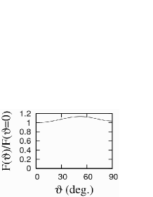
Figure 6: Plot of the free energy $f(\vartheta)$ as a function of the angle between the $c$-vector and $\mbox{\boldmath$q$}_{\perp}$. (a) The tilt angle dependence of the free energy $f(\vartheta)$. (b) Discontinuous transition is explained with the two minima at $\theta=0^{\circ}$ and $90^{\circ}$ as it should be.

The state diagram for the reduced Frank elastic moduli $\tilde{\kappa}_{1}$ and $\tilde{\kappa}_{2}$ is also calculated based on (31a). We use $\tilde{D}_{\perp}=0.5$, $\tilde{D}_{\parallel\perp}=0.01$ and $\tilde{D}_{\parallel}=0.1$. An experimental result tells that $\tilde{D}_{\parallel\perp}$ is smaller than $\tilde{D}_{\perp}$, $\tilde{D}_{\parallel}$ Martinez-Miranda et al. (1986). $\tilde{D}_{\perp}=0.5$ is about on the state boundary between $\theta=90^{\circ}$ or less, so that we would obtain the sensitive state behavior. This parameter set will be used in the following if not specified.

Effect of the Frank elastic constants is quite sensitive to $\alpha$.

(a) $\vartheta=0^{\circ}$		(b) $\vartheta=90^{\circ}$

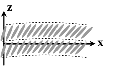
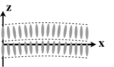
Figure 7: Layer undulation and the director configuration assuming the nonzero tilt angle $\alpha$. The splay Frank elastic energy costs at $\vartheta=0^{\circ}$ more than at $\vartheta=90^{\circ}$, because of the director component projected to the $zx$-plane.

For $\alpha\lesssim 40^{\circ}$ (Fig.5(a)), the $\theta=90^{\circ}$ state dominates except for low $\tilde{\kappa}_{2}$, while $\theta<90^{\circ}$ domain shrinks for smaller and larger $\tilde{\kappa}_{1}$. The $\theta=90^{\circ}$ state is achieved by a combination of the locking term (which is the major contribution for small $\alpha$), and the twist Frank term $|\mbox{\boldmath$N$}\cdot\left(\mbox{\boldmath$q$}_{\perp}\times\delta\mbox{\boldmath$n$}\right)|^{2}$ favoring $\mbox{\boldmath$q$}_{\perp}\parallel\mbox{\boldmath$N$}$ or $\mbox{\boldmath$q$}_{\perp}\parallel\delta\mbox{\boldmath$n$}$. The $\theta<90^{\circ}$ domain is suppressed by the two mechanisms. One for larger $\tilde{\kappa}_{1}$ is a combination of the locking term and the splay Frank term (see Fig.7 and the detailed calculation is found in Appendix C). The other for smaller $\tilde{\kappa}_{1}$ is a combination of the twist and bend Frank elastic energies, which favor $\mbox{\boldmath$q$}_{\perp}\parallel\delta\mbox{\boldmath$N$}$. For $\alpha>50^{\circ}$ (Fig.5(b)), the locking term less contributes and the anisotropic elasticity with $\tilde{D}_{\perp}$ is enhanced more. Thus both of the two minima $\mbox{\boldmath$q$}_{\perp}\parallel\mbox{\boldmath$N$}$ and $\mbox{\boldmath$q$}_{\perp}\parallel\delta\mbox{\boldmath$n$}$ are stable for higher twist $\tilde{\kappa}_{2}$. They are incompatible because of the normalization condition $\mbox{\boldmath$N$}\cdot\delta\mbox{\boldmath$n$}=0$, so the transition between $\theta=0^{\circ}$ and $\theta=90^{\circ}$ is discontinuous. This anomalous state behavior disappears for weak anisotropy (Fig.5(c)).

We also plot the free energy $f(\vartheta)$ in Fig.6. The normalization is taken with $f(\vartheta=0^{\circ})$. The minimizer $\theta$ decreases as $\alpha$ grows, but the free energy barrier is still small for $\alpha=40^{\circ}$, being a few percent of the absolute value Fig.6(a). So the equilibration to the free energy minimum might be disturbed by the internal thermal noise and an external force. However the $0^{\circ}<\theta<90^{\circ}$ state is more stable at higher $\alpha$. The discontinuous $\theta$ transition in Fig.5(c) is certainly due to the coexistence of the two local minima (Fig.6(b)).

III.5 Discussion

We next compare our calculation with the previous works. Hatwalne and Lubensky Hatwalne and Lybensky (1995) derived the elastic free energy for the Sm-C phase in a more elegant way making use of the symmetry and covariance of the model free energy. The resulting representation in the case $\mbox{\boldmath$N$}=(N_{1},0,N_{3})$ is

$$F = \frac{1}{2}\int_{\mbox{\boldmath$q$}}\left(Bq_{3}^{2}+K_{11}q_{1}^{4}+2K_{12}q_{1}^{2}q_{2}^{2}+K_{22}q_{2}^{4}\right)|u(\mbox{\boldmath$q$})|^{2}$$ (33)

We can obtain the layer compression coefficient from (11a), (29), and the normalization $\mbox{\boldmath$N$}\cdot\delta\mbox{\boldmath$n$}=0$, by setting $q_{1}=q_{2}=0$ and $q_{3}\rightarrow 0$,

$$B = \frac{8K_{3}\tilde{D}_{\perp}q_{0}^{2}}{N_{3}^{6}A}\left\{AN_{3}^{4}\left(2-N_{3}^{2}\right)-4\tilde{D}_{\perp}q_{0}^{2}\right\}.$$ (34)

We note that the layer compression elasticity stems from the director contribution $\tilde{\kappa}_{1}$ as well as the density contribution in the Sm-C phase, because a change of the layer width is associated with the change of the tilt angle.

As for the layer bending elasticity, the effective Chen-Lubensky model (31a) cannot be written in the Hatwalne-Lubensky $q$-dyadic form $(\ref{eq:FHL})$, because in general the anisotropic layer bending elasticity should be expressed as

$$F = \frac{1}{2}\int_{\mbox{\boldmath$q$}}\left(Bq_{3}^{2}+q_{\perp}^{4}K(\vartheta,\mbox{\boldmath$q$}_{\perp})\right)|u(\mbox{\boldmath$q$})|^{2}.$$ (35)

Still we can give some representations for $K_{11}$ and $K_{22}$ in the simple form,

$$K_{11} = K(\vartheta=0^{\circ})=\frac{K_{3}}{N_{3}^{2}}\left\{2\tilde{D}_{\parallel}N_{\perp}^{4}+N_{3}^{2}\left(1+\tilde{\kappa}_{1}N_{3}^{2}\right)\right\},$$ (36a)

$$K_{22} = K(\vartheta=90^{\circ})=\frac{2K_{3}\tilde{D}_{\perp}\left(\tilde{\kappa}_{1}+1\right)}{N_{3}^{2}\left(2\tilde{D}_{\perp}+\tilde{\kappa}_{1}+1\right)}.$$ (36b)

$K_{12}$ is calculated with the parabolic approximation,

$$K_{12} \simeq \frac{K({\vartheta=0^{\circ}})+K({\vartheta=90^{\circ}})}{2}-\frac{1}{4}\left(\left.\frac{\partial K}{\partial x}\right|_{\vartheta=0^{\circ}}-\left.\frac{\partial K}{\partial x}\right|_{\vartheta=90^{\circ}}\right)$$ (37)

The three elastic constants $K_{11}$, $K_{12}$, and $K_{22}$ contain both the density and the director contributions as pointed out in the previous research Hatwalne and Lybensky (1995).

In this way, we bridge the models of smectic liquid crystal at different coarse-graining levels. It leads one to a quantitative discussion with the phenomenological macroscopic model Hatwalne and Lybensky (1995), based on the experimental determination of the Chen-Lubensky model Martinez-Miranda et al. (1986).

We conclude this section comparing our results for Sm-C liquid crystals with other layer forming materials. Diblock copolymers, chemically connected two different homopolymers, do not possess the definite molecular orientational degree of freedom especially in the weak segregation regime Leibler (1980). Thus anisotropic elasticity cannot occur. On the other hand, in surfactant systems, the linear amphiphilic molecule is basically normal to the surfactant layer Gompper and Klein (1992); Chen et al. (1990). This is similar to the Sm-A phase of liquid crystals rather than the Sm-C phase. Thus amphiphilic system again would not have an in-plane anisotropic coupling. However in some cases the surfactant molecules may be aligned at a nonzero tilt angle against the layer normal Safran et al. (1986); Wang and Gong (1996); Kuhn and Rehage (2000). Such systems might have an anisotropic layer elasticity as in the present Sm-C liquid crystal case.

IV Hydrodynamics of Smectic-C layers

In this section, we consider the transverse wave in smectic liquid crystals which oscillates in the layer normal direction, and travels perpendicularly to the layer normal. The wave frequency is much lower than the inverse of the molecular time scale ($\sim 10^{8}$Hz), so that the permeation effect which changes the layer width is negligible de Gennes and Prost (1994). Also we eliminate some rapidly relaxed degrees of freedom, namely the density $\rho$, the local energy $\epsilon$, the velocity along the layer in-plane directions, the pressure $P$, and the $c$-vector in the time scale $\sim 10^{-4}$s.

We derive the equation of motion of $u(\mbox{\boldmath$r$})$ from the time evolution of the velocity field $\mbox{\boldmath$v$}(\mbox{\boldmath$r$})$. According to the unified hydrodynamic description de Gennes and Prost (1994); Martin et al. (1972), a set of the hydrodynamic equations at a constant temperature with no external field is

$$\nabla\cdot{\mbox{\boldmath$v$}(\mbox{\boldmath$r$})} = 0,$$ (38a)

$$\frac{\partial u(\mbox{\boldmath$r$})}{\partial t}-v_{z}(\mbox{\boldmath$r$}) = 0,$$ (38b)

$$-B_{z\beta\gamma}\partial_{\gamma}v_{\beta}(\mbox{\boldmath$r$}) = -\nu h_{z}(\mbox{\boldmath$r$}),$$ (38c)

$$\rho_{0}\frac{\partial v_{z}(\mbox{\boldmath$r$})}{\partial t} = -\frac{\delta F}{\delta u}-B_{zz\beta}\partial_{\beta}h_{z}(\mbox{\boldmath$r$})+\eta_{z\beta\gamma\delta}\partial_{\gamma}\partial_{\delta}v_{\beta}(\mbox{\boldmath$r$}),$$ (38d)

where $h_{z}$ is the torque acting on the $c$-vector and $B_{\alpha\beta\gamma}$ is the coupling constant between the torque and the velocity. The first equation is the incompressibility condition originated from the equation of continuity. The second and third equation describes the relaxation of the layer permeation and the rotational $c$-vector mode respectively. The last equation is derived from the momentum conservation essentially equivalent to the Navier-Stokes equation. From the above equations, we derive the equation of motion as

$$\rho_{0}\frac{\partial^{2}u(\mbox{\boldmath$r$})}{\partial t^{2}} = \mu_{\beta\gamma}\partial_{\beta}\partial_{\gamma}\frac{\partial u(\mbox{\boldmath$r$})}{\partial t}-\frac{\delta F}{\delta u}.$$ (39)

In the smectic-C phase, the model free energy has the static elastic coupling of the layer displacement field $u(\mbox{\boldmath$r$})$ and $c$-vector. Here exists the dynamical viscous coupling of the velocity and the molecular orientation in the first term of (39). Anisotropic viscosity tensor $\mu_{\beta\gamma}$ ($\beta$, $\gamma$=1, 2) depends on the $c$-vector, as

$$\mu_{\beta\gamma} = \mu_{0}\,\delta_{\beta\gamma}+\mu_{1}n_{\beta}(\mbox{\boldmath$r$})n_{\gamma}(\mbox{\boldmath$r$}),$$ (40)

where $\mu_{0}$ and $\mu_{1}$ are constants. The isotropic and rotational viscosities are reported to be of the same order ($\sim 1$ Poise) in the experimental studies Tamamushi (1974); Meiboom and Hewitt (1975). We then add an oscillatory source term $s(\mbox{\boldmath$r$},t)$. We consider the oscillating wall and cylindrical sources $s(\mbox{\boldmath$r$},t)=s_{0}\cos(\omega t)\delta(x)$ and $s_{0}\cos(\omega t)\delta(x)\delta(y)$ respectively, to examine the anisotropy in the Sm-C phase (Fig.8). This vibrating force can be provided by an oscillatory object, for example, an electric field Pieranski et al. (1993).

(a)		(b)

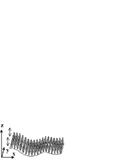
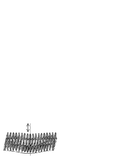
Figure 8: Illustration of the oscillatory sources. We consider the two geometries: (a) the one-dimensional wall and (b) the two-dimensional cylinder at the center point of the layer plane.

The linearized dynamic equation in Fourier space is

$$\rho_{0}\frac{\partial^{2}u(\mbox{\boldmath$q$},t)}{\partial t^{2}} = -\left[(\mu_{0}\,\delta_{\beta\gamma}+\mu_{1}N_{\beta}N_{\gamma})q_{\beta}q_{\gamma}\frac{\partial}{\partial t}+\left(Bq_{\parallel}^{2}+K(\vartheta)q_{\perp}^{4}\right)\right]u(\mbox{\boldmath$q$},t)+s(\mbox{\boldmath$q$},t),$$ (41)

where $s(\mbox{\boldmath$q$},t)=4\pi^{2}s_{0}\cos(\omega t)\delta^{(2)}(\mbox{\boldmath$q$}_{\perp})$ and $2\pi s_{0}\cos(\omega t)\delta(q_{z})$ is the one-dimensional wall and two-dimensional cylindrical source respectively. The thermodynamic force $\delta F/\delta u^{*}$ is written in the linear form $L(\mbox{\boldmath$q$})u(\mbox{\boldmath$q$},t)=\left(Bq_{\parallel}^{2}+K(\vartheta,\mbox{\boldmath$q$}_{\perp})q_{\perp}^{4}\right)u(\mbox{\boldmath$q$},t)$.

We next derive the dimensionless dynamic equation. The characteristic parameter set is listed in Table 2.

Table 2: Parameters and their typical scales in the dynamic equation (41) de Gennes and Prost (1994); Tamamushi (1974); Chen and Jasnow (2000); Meiboom and Hewitt (1975).

parameter	description	typical scale
$\rho_{0}$	averaged molecular density	$\sim 1$g$/$cm3
$u(\mbox{\boldmath$r$})$	layer displacement field	$\sim 10^{-7}-10^{-8}$cm
$\mu_{0}$	isotropic viscosity	$\sim 1$ Poise
$\mu_{1}$	rotational viscosity	$\sim 1$ Poise
$q_{i}$	undulation wave number	$\sim 10^{-5}$cm
$\omega$	undulation frequency	$\sim 10^{4}$Hz
$B=C_{i}\Psi_{0}^{2}q_{0}^{2}\,(i=\perp,\parallel)$	layer compression elastic constant	$\sim 10^{6}$dyn$/$cm2
	(second order density elastic constant)
$D_{i}\Psi_{0}^{2}q_{0}^{2}\,(i=\perp,\perp\parallel,\parallel)$	layer bending elastic constant	$\sim 10^{-6}$dyn
	(fourth order density elastic constant)
$K_{i}\,(i=1,2,3)$	Frank elastic modulus	$\sim 10^{-6}$dyn

The reduced dynamic equation is

$$\frac{\rho_{0}\xi^{4}}{K_{3}\tau^{2}}\frac{\partial^{2}\tilde{u}(\tilde{\mbox{\boldmath$q$}},\tilde{t})}{\partial\tilde{t}^{2}} = -\frac{\xi^{2}\eta_{c}}{K_{3}\tau}\left(\tilde{\eta}_{0}\tilde{q}^{2}+\tilde{\eta}_{1}\left(\mbox{\boldmath$N$}\cdot\tilde{\mbox{\boldmath$q$}}\right)^{2}\right)\frac{\partial\tilde{u}(\tilde{\mbox{\boldmath$q$}},\tilde{t})}{\partial\tilde{t}}$$ (42)

$$-\left(\frac{B_{0}}{K_{3}q_{0}^{2}}\tilde{B}\tilde{q}_{z}^{2}+\tilde{K}(\vartheta)\tilde{q}^{4}\right)\tilde{u}(\tilde{\mbox{\boldmath$q$}},\tilde{t})+\frac{\xi^{4}q_{0}}{K_{3}}s(\tilde{\mbox{\boldmath$q$}},\tilde{t}),$$

where we introduced the dimensionless valuables $t=\tau\tilde{t}$, $\omega\tau=\tilde{\omega}$, $uq_{0}=\tilde{u}$, $q_{i}\xi=\tilde{q}_{i}$, $\eta_{i}=\eta_{c}\tilde{\eta}_{i}\,\,(i=0,1)$, $B=B_{0}\tilde{B}$ and $K(\vartheta)=K_{3}\tilde{K}(\vartheta)$. All the dimensionless constants are of order $\sim 1$. We set the characteristic scales according to Table 2: $\tau=10^{-4}$s, $\xi=10^{-5}$cm, $\eta_{c}=1$ Poise and $B_{0}=10^{6}$dyn$/$cm². In this parameter set, the scale of each term in (42) is $\rho_{0}\xi^{4}/K_{3}\tau^{2}\sim 10^{-6}$ and $\xi^{2}\eta_{c}/K_{3}\tau\sim B_{0}/K_{3}q_{0}^{2}\sim 1$. Thus the inertia term can be neglected and the final form of the dimensionless dynamic equation is

$$\tilde{\zeta}\frac{\partial\tilde{u}(\tilde{\mbox{\boldmath$q$}},\tilde{t})}{\partial\tilde{t}}+\tilde{L}(\tilde{\mbox{\boldmath$q$}})\tilde{u}(\tilde{\mbox{\boldmath$q$}},\tilde{t})=\tilde{s}(\tilde{\mbox{\boldmath$q$}},\tilde{t}),$$ (43)

where the effective viscosity $\tilde{\zeta}=\tilde{q}^{2}\left(\tilde{\eta}_{0}+\tilde{\eta}_{1}\cos^{2}\vartheta\right)$, and the normalized external force $\tilde{s}$ is given by $\tilde{s}=\tilde{s}_{0}(\tilde{\mbox{\boldmath$q$}})\cos(\tilde{\omega}\tilde{t})$. The reduced amplitude $\tilde{s}_{0}$ is $4\pi^{2}s_{0}q_{0}\xi^{4}\delta(q_{y})\delta(q_{z})/K_{3}$ and $2\pi s_{0}q_{0}\xi^{4}\delta(q_{z})/K_{3}$ in the oscillatory wall and the vibrating cylinder case respectively. The time evolution is

$$\tilde{u}(\tilde{\mbox{\boldmath$q$}},\tilde{t})=\frac{\tilde{s}_{0}}{\tilde{\zeta}\left(\tilde{\lambda}^{2}+\tilde{\omega}^{2}\right)}\left(-\tilde{\lambda}\cos\tilde{\omega}\tilde{t}+\tilde{\omega}\sin\tilde{\omega}\tilde{t}+\tilde{\lambda}\exp\tilde{\lambda}\tilde{t}\right),$$ (44)

where $\tilde{\lambda}=-\tilde{L}/\tilde{\zeta}$ and the initial condition is set to be $\tilde{u}(\tilde{\mbox{\boldmath$q$}},0)=0$.

Visualization of the wave propagation is depicted in Fig.9 and Fig.10. Unphysical infinite wavelength mode is excluded. We use the parameter set: $\tilde{C}_{\parallel}=4\times 10^{12}$cm^-2, $\tilde{D}_{\perp}=\tilde{D}_{\parallel\perp}=\tilde{D}_{\parallel}=0.1$, $\tilde{\kappa}_{1}=\tilde{\kappa}_{2}=0$, $\omega=5\times 10^{4}$Hz, and $\alpha=30^{\circ}$. The reference $c$-vector is tilted against the $x$-axis at $40^{\circ}$. The same parameter set is used in the following if not specified. The layer displacement is shown with the brightness, and the director change is indicated with the unit arrow. The dumped director degree of freedom is governed by the layer displacement field through (29). While the layer displacement scale is $\sim 10^{-7}$cm^-1, the director rotation angle is about $10^{-3}-10^{-4}$rad, which can be observed in experiment Galerne (1981); Kuo et al. (2006).

In Fig.9, the planar oscillation orientates the director with the layer displacement. Anisotropic wave propagation is obvious under a cylindrical source (Fig.10). The favored angle is $\theta=90^{\circ}$, as in the experimental study Johnson and Saupe (1977) and the free energy analysis (Fig.4). The wave velocity is faster in the rigid direction $\mbox{\boldmath$c$}\parallel\mbox{\boldmath$q$}_{\perp}$, than in the soft orientation $\mbox{\boldmath$c$}\perp\mbox{\boldmath$q$}_{\perp}$. A simple dimensional analysis of (43) with $\tilde{s}=0$ gives the ratio

$$v_{\parallel}/v_{\perp}=\left(\tilde{K}(0^{\circ})/\tilde{K}(90^{\circ})\right)^{\frac{1}{2}}\left\{\tilde{\eta}_{0}/\left(\tilde{\eta}_{0}+\tilde{\eta}_{1}\right)\right\}^{\frac{1}{2}}.$$ (45)

We conclude this section with the remark that both the director alignment and the anisotropic wave propagation are entirely controlled by the static and dynamic coupling between the layer displacement and the director (45), and could be observed within the experimental resolution.

		(a) $t=1.2\times 10^{-4}$s	(b) $t=1.8\times 10^{-4}$s
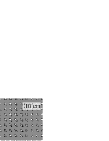
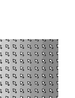
		(c) $t=2.4\times 10^{-4}$s	(d) $t=3.0\times 10^{-4}$s

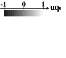
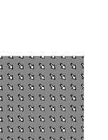
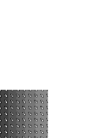
Figure 9: Snapshots of the layer oscillation under a planar source ($x=0$). The brightness indicates the local layer displacement and the unit arrow represents the deviation of the director from the ground state. We set $\tilde{C}_{\parallel}=4\times 10^{12}$cm^-2, $\tilde{D}_{\perp}=\tilde{D}_{\parallel\perp}=\tilde{D}_{\parallel}=0.1$, $\tilde{\kappa}_{1}=\tilde{\kappa}_{2}=0$, $\omega=5\times 10^{4}$Hz, and $\alpha=30^{\circ}$.

		(a) $t=1.2\times 10^{-4}$s	(b) $t=1.8\times 10^{-4}$s
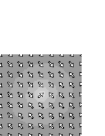
		(c) $t=2.4\times 10^{-4}$s	(d) $t=3.0\times 10^{-4}$s

Figure 10: Anisotropic wave propagation is shown in the presence of an isotropic oscillatory source ($x=y=0$). The wave front is elliptic with the long axis parallel to the reference director $c$.

V Conclusion

In this paper, we analytically derived the effective generalized Chen-Lubensky model by adiabatic elimination of the director relaxation. For Sm-A phase, the director unlocking from the layer normal is confirmed at an undulation wavelength shorter than the director coherent length. The effective layer bending elastic modulus is written as a function of the unlocking angle $\alpha$, and decays with the increase of $\alpha$. This agrees with the argument in the previous work Ogawa and Uchida (2006). In Sm-C phase, on the other hand, not only the director unlocking but anisotropic elasticity arises from the $c$-vector. After the detailed study, it turned out that the preferred angle $\theta$ between the layer bending orientation and the $c$-vector varies from $0^{\circ}$ to $90^{\circ}$ depending on the layer elastic constants, the Frank constants, the tilt angle, and the undulation wavelength. Transitions between the different $\theta$ states are not only continuous but also discontinuous. Then the new characteristic length $\lambda_{A}$ is found, which plays an important role on the elasticity of Sm-C phase. The model parameters of the macroscopic free energy  Hatwalne and Lybensky (1995) are determined from the more microscopic Chen-Lubensky model. It allows a quantitative argument based on the model  Hatwalne and Lybensky (1995) with the experimental determination of the model parameters Martinez-Miranda et al. (1986). We also compared smectic liquid crystals with other layer forming materials.

Next we discussed the hydrodynamics of Sm-C layers using the effective elastic energy derived above. We derive the Sm-C hydrodynamics with the director deformation eliminated. Anisotropic wave propagation from the isotropic oscillatory source and the director orientation in the simple undulation along one direction are confirmed. These effect could be observed in experiment  Pieranski et al. (1993); Galerne (1981); Kuo et al. (2006). By converting the mechanical undulation to the optical information through the director orientation, here also arises a new possible application of liquid crystals for a sensitive mechanical sensor.

Appendix A Effective layer bending elastic modulus as a function of $m$-$n$ unlocking angle

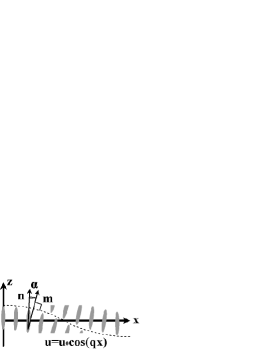
Figure 11: Schematic representation of the smectic layer with a sinusoidal undulation. Here exists the small unlocking angle $\alpha$ between the layer normal $m$ and the director $n$, which accounts for the weak bending elastic modulus.

Here we give a better representation of the effective layer bending elastic modulus (9), as a function of the root mean square (RMS) of the angle $\tilde{\alpha}$ between the layer normal and the director. This leads us to a more quantitative understanding of the previous numerical result on the mean curvature of smectic layers in the TGB phase Ogawa and Uchida (2006).

We suppose a single Fourier mode of the layer undulation $u(\mbox{\boldmath$r$})=u_{0}\cos(qx)$ (Fig.11). The wave-number vector is along the $x$-axis. With the help of (6), $m$ and $n$ are

$$n_{x} = \frac{1}{1+(\lambda q)^{2}}qu_{0}\sin(qx),$$ (46a)

$$m_{x} = qu_{0}\sin(qx),$$ (46b)

$$n_{y} = m_{y}=0,$$ (46c)

$$n_{z} = m_{z}=1.$$ (46d)

In a small deformation, the tilt angle $\alpha$ is given by

$$\alpha \simeq m_{x}-n_{x}=\frac{(\lambda q)^{2}}{1+(\lambda q)^{2}}qu_{0}\sin(qx).$$ (47)

The RMS $\tilde{\alpha}$ is readily calculated

$$\tilde{\alpha}=\frac{1}{\sqrt{2}}\frac{u_{0}\lambda^{2}q^{3}}{1+(\lambda q)^{2}}\simeq\frac{1}{\sqrt{2}}u_{0}\lambda^{2}q^{3},$$ (48)

where the smooth undulation condition $q\ll\lambda^{-1}$ is assumed in the last line. We note that the tilt angle is roughly proportional to the cube of the wave-number, and the characteristic length is a combination of the penetration length and the undulation amplitude $\left(\lambda^{2}u_{0}\right)^{1/3}$. Thus the effective layer bending rigidity is now written as a function of $\tilde{\alpha}$

$$\tilde{\kappa}\left(\tilde{\alpha}\right)=\frac{1}{1+\left(\sqrt{2}\tilde{\alpha}\lambda/u_{0}\right)^{2/3}}.$$ (49)

The same method could be applied for the Sm-A phase also in the Chen-Lubensky model.

Appendix B Derivation of $\tilde{D}_{\perp}\tilde{D}_{\parallel}-\tilde{D}_{\parallel\perp}^{2}>0$ and one constant approximation

Here we prove the relation $\tilde{D}_{\perp}\tilde{D}_{\parallel}-\tilde{D}_{\parallel\perp}^{2}>0$ to guarantee the convexity of the effective free energy as a function of $x=\cos^{2}\vartheta$ in the one Frank constant case (53). This relation actually holds for an arbitrary set of Frank elastic moduli, because the inequality is based on the stability of the smectic layer. With the density profile $\Psi=\Psi_{0}\exp(\mbox{\boldmath$q$}\cdot\mbox{\boldmath$r$})$, the $q$-dependent part of the Chen-Lubensky Hamiltonian (11a) is proportional to

$$\int d\mbox{\boldmath$r$}\Psi_{0}^{2}\left[\tilde{D}_{\parallel}Q_{\parallel}^{4}+2\tilde{D}_{\parallel\perp}Q_{\parallel}^{2}Q_{\perp}^{2}+\tilde{D}_{\perp}Q_{\perp}^{4}\right],$$ (50)

where the effective momenta $Q_{\parallel}^{2}=(q_{\parallel}-q_{0})^{2}+q_{0\parallel}^{2}$ and $Q_{\perp}^{2}=q_{\perp}^{2}-q_{0\perp}^{2}$, the characteristic wave number $q_{0\parallel}^{2}=\left(\tilde{C}_{\parallel}\tilde{D}_{\perp}-\tilde{C}_{\perp}\tilde{D}_{\parallel\perp}\right)/\left[2\left(\tilde{D}_{\perp}\tilde{D}_{\parallel}-2\tilde{D}_{\parallel\perp}\right)\right]$ and $q_{0\perp}^{2}=\left(\tilde{C}_{\parallel}\tilde{D}_{\parallel\perp}-\tilde{C}_{\perp}\tilde{D}_{\parallel}\right)/\left[2\left(\tilde{D}_{\perp}\tilde{D}_{\parallel}-2\tilde{D}_{\parallel\perp}^{2}\right)\right]$, and the projected wave-number vector $\mbox{\boldmath$q$}_{\parallel}=(\mbox{\boldmath$n$}\cdot\mbox{\boldmath$q$})\mbox{\boldmath$n$}$, $\mbox{\boldmath$q$}_{\perp}=-\mbox{\boldmath$n$}\times\left(\mbox{\boldmath$n$}\times\mbox{\boldmath$q$}\right)$ are utilized. Positive definiteness of (50) requires

$$\tilde{D}_{\perp}\tilde{D}_{\parallel}-\tilde{D}_{\parallel\perp}^{2} > 0.$$ (51)

This inequality helps one to prove a convexity of the free energy at the one constant approximation ($K_{1}=K_{2}=K_{3}$). In this case, the free energy is simplified as

$$\frac{\tilde{D}_{\perp}N_{3}^{2}}{q_{\perp}^{4}|u(\mbox{\boldmath$q$})|^{2}}\tilde{f} = 2N_{\perp}^{4}\left(\tilde{D}_{\parallel}\tilde{D}_{\perp}-\tilde{D}_{\parallel\perp}^{2}\right)x^{2}+\tilde{D}_{\perp}\left(1-N_{\perp}^{2}x\right)+2\tilde{D}_{\parallel\perp}N_{\perp}^{2}x$$

$$-\frac{\left(2N_{\perp}^{2}+k_{\perp}^{2}\right)\left(-2N_{\perp}^{4}\tilde{D}_{\parallel\perp}^{2}x^{2}+\tilde{D}_{\perp}\left(1-N_{\perp}^{2}x\right)+2\tilde{D}_{\parallel\perp}N_{\perp}^{2}x\right)-2N_{3}^{2}N_{\perp}^{2}\tilde{D}_{\perp}x}{2k_{\perp}^{2}\tilde{D}_{\perp}\left(1-N_{\perp}^{2}x\right)+4\tilde{D}_{\perp}N_{\perp}^{2}\left(1-x\right)+2N_{\perp}^{2}+k_{\perp}^{2}},$$

and the second derivative is

$$\frac{N_{3}^{2}\tilde{D}_{\perp}}{4N_{\perp}^{4}q_{\perp}^{4}|u(\mbox{\boldmath$q$})|^{2}}\tilde{f}^{{}^{\prime\prime}}(x) = \tilde{D}_{\parallel}\tilde{D}_{\perp}-\tilde{D}_{\parallel\perp}^{2}+\frac{2N_{\perp}^{2}+k_{\perp}^{2}}{\left\{\left(1+2\tilde{D}_{\perp}\right)\left(2N_{\perp}^{2}+k_{\perp}^{2}\right)-2N_{\perp}^{2}\tilde{D}_{\perp}\left(k_{\perp}^{2}+2\right)x\right\}^{3}}$$ (53)

$$\times\left\{\left(1+2\tilde{D}_{\perp}\right)\left(2N_{\perp}^{2}+k_{\perp}^{2}\right)\tilde{D}_{\parallel\perp}-\left(k_{\perp}^{2}+2\right)\tilde{D}_{\perp}\right\}^{2},$$

where the dimensionless wave number is given by $k_{\perp}(\tilde{D}_{\parallel\perp},\tilde{D}_{\perp})\equiv\lambda_{A}q_{\perp}$.

Appendix C Splay Frank energy as a function of $\vartheta$

We calculate the splay energy for a small tilt angle $\alpha$ and the angle $\vartheta$ between $c$ and $\mbox{\boldmath$q$}_{\perp}$. Let the $x$-axis be parallel to $\mbox{\boldmath$q$}_{\perp}$. The director is $\mbox{\boldmath$n$}=\left(\sin\alpha\cos\vartheta,\sin\alpha\sin\vartheta,\cos\alpha\right)$. Assuming the smooth layer undulation $q_{\perp}\ll\lambda^{-1}$, the director deformation perfectly follows the layer normal vector. Undulated director configuration is obtained by operating the rotation matrix about the $y$-axis $\mbox{\boldmath$R$}_{y}$

$$\mbox{\boldmath$R$}_{y}=\left(\begin{array}[]{c c c}\cos qx&0&-\sin qx\\ 0&1&0\\ \sin qx&0&\cos qx\end{array}\right),$$ (57)

to the reference director $n$. Thus the spatially averaged splay energy is expressed as

$$\left\langle\left\{\nabla\cdot{\left(\mbox{\boldmath$R$}_{y}\mbox{\boldmath$n$}\right)}\right\}^{2}\right\rangle=\frac{q^{2}}{2}\left(\sin^{2}\alpha\cos^{2}\vartheta+\cos^{2}\alpha\right).$$ (58)

Stability of the $\theta=90^{\circ}$ state grows as the splay Frank elasticity dominates. However this effect of the splay term is not very strong, due to the factor $\sin^{2}\alpha$.

References

- de Gennes and Prost (1994) P. G. de Gennes and J. Prost, The Physics of Liquid Crystals (Clarendon, Oxford, 1994).
- Chainkin and Lubensky (1995) P. M. Chainkin and T. C. Lubensky, Principles of Condensed Matter Physics (Cambridge University Press, Cambridge, England, 1995).
- Keyes et al. (1973) P. H. Keyes, H. T. Weston, and W. B. Daniels, Phys. Rev. Lett. 31, 628 (1973).
- Aharony et al. (1986) A. Aharony, R. J. Birgeneau, J. D. Brock, and J. D. Litster, Phys. Rev. Lett. 57, 1012 (1986).
- Shashidhar et al. (1984) R. Shashidhar, B. R. Ratna, and S. K. Prasad, Phys. Rev. Lett. 53, 2141 (1984).
- Drossinos and Ronis (1986) Y. Drossinos and D. Ronis, Phys. Rev. A 33, 589 (1986).
- de Gennes (1973) P. G. de Gennes, Mol. Cryst. Liq. Cryst. 21, 49 (1973).
- Chu and McMillan (1977) K. C. Chu and W. L. McMillan, Phys. Rev. A 15, 1181 (1977).
- Chen and Lubensky (1976) J. Chen and T. C. Lubensky, Phys. Rev. A 14, 1202 (1976).
- Benguigui (1979) L. Benguigui, J. Phys. (Paris). Colloq. 40, C3 (1979).
- Huang and Lien (1981) C. C. Huang and S. C. Lien, Phys. Rev. Lett. 47, 1917 (1981).
- Grinstein and Toner (1983) G. Grinstein and J. Toner, Phys. Rev. Lett. 26, 2386 (1983).
- Witanachchi et al. (1983) S. Witanachchi, J. Huang, and J. T. Ho, Phys. Rev. Lett. 50, 594 (1983).
- Safinya et al. (1983) C. R. Safinya, L. J. Martinez-Miranda, M. Kaplan, J. D. Litster, and R. J. Birgeneau, Phys. Rev. Lett. 50, 56 (1983).
- Martinez-Miranda et al. (1986) L. J. Martinez-Miranda, A. R. Kortan, and R. J. Birgeneau, Phys. Rev. Lett. 56, 2264 (1986).
- Kitzerow and Bahr (2002) H. S. Kitzerow and C. Bahr, eds., Chirality in Liquid Crystals (Springer-Verlag, New York, 2002).
- de Gennes (1972) P. G. de Gennes, Solid State Commun. 10, 753 (1972).
- Renn and Lubensky (1988) S. R. Renn and T. C. Lubensky, Phys. Rev. A 38, 2132 (1988).
- Goodby et al. (1989) J. W. Goodby, M. A. Waugh, S. M. Stein, E. Chin, R. Pindak, and J. S. Patel, Nature 337, 449 (1989).
- Lubensky and Renn (1990) T. C. Lubensky and S. R. Renn, Phys. Rev. A 41, 4392 (1990).
- Ismaili et al. (2000) M. Ismaili, A. Anakkar, G. Joly, and N. Isaert, Phys. Rev. E 61, 519 (2000).
- Grelet et al. (2001a) E. Grelet, B. Pansu, M. Li, and H. T. Nguyen, Phys. Rev. Lett. 86, 3791 (2001a).
- DiDonna and Kamien (2002) B. A. DiDonna and R. D. Kamien, Phys. Rev. Lett. 89, 215504 (2002).
- Yamamoto et al. (2005) J. Yamamoto, I. Nishiyama, M. Inoue, and H. Yokoyama, Nature 437, 525 (2005).
- Ogawa and Uchida (2006) H. Ogawa and N. Uchida, Phys. Rev. E 73, 060701(R) (2006).
- Grelet et al. (2001b) E. Grelet, B. Pansu, and H. T. Nguyen, Phys. Rev. E 64, 010703(R) (2001b).
- Ohta and Kawasaki (1986) T. Ohta and K. Kawasaki, Macromol. 19, 2621 (1986).
- Gompper and Klein (1992) G. Gompper and S. Klein, J. Phys. II (France) 2, 1725 (1992).
- Leibler (1980) L. Leibler, Macromol. 13, 1602 (1980).
- Hatwalne and Lybensky (1995) Y. Hatwalne and T. C. Lybensky, Phys. Rev. E 52, 6240 (1995).
- Martin et al. (1972) P. C. Martin, O. Parodi, and P. S. Pershan, Phys. Rev. A 6, 2401 (1972).
- Buka and Kramer (1996) A. Buka and L. Kramer, eds., Pattern Formation in Liquid Crystals (Springer New York, 1996).
- Pargellis et al. (1992) A. N. Pargellis, P. Finn, J. W. Goodby, P. Panizza, B. Yurke, and P. E. Cladis, Phys. Rev. A 46, 7765 (1992).
- Carlsson et al. (1995) T. Carlsson, F. M. Leslie, and N. A. Clark, Phys. Rev. E 51, 4509 (1995).
- Johnson and Saupe (1977) D. Johnson and A. Saupe, Phys. Rev. A 15, 2079 (1977).
- Cladis et al. (1985) P. E. Cladis, Y. Couder, and H. R. Brand, Phys. Rev. Lett. 55, 2945 (1985).
- Chevallard et al. (1997) C. Chevallard, T. Fisch, and J. M. Gilli, J. Phys. II (France) 7, 1261 (1997).
- Clark (1979) N. Clark, Appl. Phys. Lett. 35, 688 (1979).
- Clark and Meyer (1973) N. Clark and R. B. Meyer, Appl. Phys. Lett. 22, 493 (1973).
- Yablonskii et al. (2003) S. V. Yablonskii, K. Nakano, M. Ozaki, and K. Yoshino, JETP Lett. 77, 140 (2003).
- Uto et al. (1997) S. Uto, E. Tazoh, M. Ozaki, and K. Yoshino, J. Appl. Phys. 82, 2791 (1997).
- Luk’yanchuk (1998) I. Luk’yanchuk, Phys. Rev. E 57, 574 (1998).
- Kundagrami and Lubensky (2003) A. Kundagrami and T. C. Lubensky, Phys. Rev. E 68, 060703 (2003).
- Navailles et al. (1995) L. Navailles, R. Pindak, P. Barois, and H. T. Nguyen, Phys. Rev. Lett. 74, 5224 (1995).
- Meiboom and Hewitt (1975) A. Meiboom and R. C. Hewitt, Phys. Rev. Lett. 34, 1146 (1975).
- Chen et al. (1990) K. Chen, C. Jayaprakash, R. Pandit, and W. Wenzel, Phys. Rev. Lett. 65, 2736 (1990).
- Safran et al. (1986) S. A. Safran, M. O. Robbins, and S. Garoff, Phys. Rev. A 33, 2186 (1986).
- Wang and Gong (1996) Z. Wang and C. Gong, Phys. Rev. B 54, 17067 (1996).
- Kuhn and Rehage (2000) H. Kuhn and H. Rehage, Phys. Chem. Chem. Phys. 2, 1023 (2000).
- Tamamushi (1974) B. Tamamushi, Rheol. Acta 13, 247 (1974).
- Pieranski et al. (1993) P. Pieranski, L. Beliard, J.-P. Tournellec, X. Leoncini, C. Furtlehner, H. Dumoulin, E. Riou, B. Jouvin, J.-P. Fénerol, P. Palaric, et al., Physica A 194, 364 (1993).
- Chen and Jasnow (2000) H.-Y. Chen and D. Jasnow, Phys. Rev. E 61, 493 (2000).
- Galerne (1981) Y. Galerne, Phys. Rev. A 24, 2284 (1981).
- Kuo et al. (2006) L.-Y. Kuo, K.-L. Lee, and J.-J. Wu, Jpn. J. Appl. Phys. 45, 8775 (2006).