Boron in copper: a perfect misfit in the bulk and cohesion enhancer at a grain boundary

Abstract

Our ab initio  study suggests that boron segregation to the $\Sigma 5$(310)[001] grain boundary should strengthen the boundary up to 1.5 ML coverage (15.24 at/nm²). The maximal effect is observed at 0.5 ML and corresponds to boron atoms filling exclusively grain boundary interstices. In copper bulk, B causes significant distortion both in interstitial and regular lattice sites for which boron atoms are either too big or too small. The distortion is compensated to large extent when the interstitial and substitutional boron combine together to form a strongly bound dumbell. Our prediction is that bound boron impurities should appear in sizable proportion if not dominate in most experimental conditions. A large discrepancy between calculated heats of solution and experimental terminal solubility of B in Cu is found, indicating either a sound failure of the local density approximation or, more likely, strongly overestimated solubility limits in the existing B–Cu phase diagram.

Introduction

Boron has an extremely good record in improving intergranular cohesion in metals. It is mostly famous for curing the long standing problem of room temperature brittleness in Ni₃Al.Liu et al. (1985) Boron segregation was found to reinforce grain boundaries in other intermetallic compounds (FeAl, NiAl, Ni₃Si) and to improve low temperature ductility in bcc iron and refractory metals, such as Mo and W (see, e.g., Ref. [Lejček and Fraczkiewicz, 2003] and references therein).

The effect of boron addition on copper is far less studied. According to the Cu–B phase diagram,Massalski (1996) boron solubility in copper is low, 0.06 at.% at room temperature rising to 0.29 at.% at the eutectic temperature 1013 ${}^{\circ}\mathrm{C}$. Dissolved boron has a strong propensity to segregate to surfaces and interfaces. It is not clear whether segregation weakens or strengthen grain boundaries. Nevertheless, doping copper with boron is found to be efficient in preventing segregation of antimony to grain boundaries.Glikman et al. (1974) Substantial improvement of mechanical properties of nanocrystalline Cu samples is reported as B segregation can be used to limit grain growth during heat treatment.Suryanarayanan et al. (1999) Despite such encouraging experimental findings, quite surprisingly, no theoretical simulations of boron at copper grain boundaries or even free surfaces, are known to us.

Similarly poor is the situation with studies of boron in bulk copper. It is not even clear whether boron occupies interstitial or substitutional positions. Analysis of boron’s neighbours in the Periodic Table does not rule out either possibility. Carbon is an interstitial impurity in Cu,Ellis et al. (1999) whereas Al and Be are substitutional impurities. In recent experimental work in which accelerated boron ions were implanted in Cu, both types of impurities were observed.Füllgrabe et al. (2001)

In the present study we employ standard density functional calculations to study the behaviour of boron impurities at a copper grain boundary and in the bulk. We find that boron strengthens the $\Sigma 5${310}[001] symmetric tilt grain boundary in the whole range of boundary coverages investigated (up to 1.5 ML). The maximum strengthening occurs at 0.5 ML at which boron exclusively occupies grain boundary interstices. We further identify mechanisms responsible for grain boundary strengthening within the framework of the “ghost impurity cycle” proposed in our previous work.Lozovoi et al. (2006) The cycle admits the occupation of both substitutional and interstitial positions by impurity atoms at the interface, a feature that is fully exploited in the present study.

Due to the peculiar interplay of atomic sizes, interstitial and substitutional positions are equally unwelcoming to boron in bulk Cu. Boron is too big an interstitial impurity and too small a substitutional impurity. As a result, both have nearly the same heat of solution with the interstitial position marginally preferred. If, however, B atoms combine in dumbells then most of the elastic distortion of the host is eliminated and significant lowering of the heat of solution is achieved. The energy gain is so large that boron dumbells should persist up to high temperatures. Another surprising finding of our study is a large disagreement between the theoretical heat of solution and experimentally observed maximal solubility of B in Cu.

The paper is organised as follows. Sec. I outlines definitions and thermodynamical relations used in the present work. The computational setup is described in Sec. II. The results on B in bulk Cu are presented in Sec. III, whereas Sec. IV is concerned with the effect of boron at the grain boundary. In the latter section, we first look at the change of the work of separation and at the impurity segregation energies (Sec. IV.1), then we discuss atomic structure of the boundaries and free surfaces with different boron content (Sec. IV.2), and finally apply the “ghost impurity cycle” to reveal the mechanisms responsible for the cohesion enhancement (Sec. IV.3). Our main findings are summarised in Sec. V. A thermodynamic model used to estimate the concentration of different kinds of boron impurity in bulk copper, is outlined in the Appendix.

I Work of separation and ghost impurity cycle

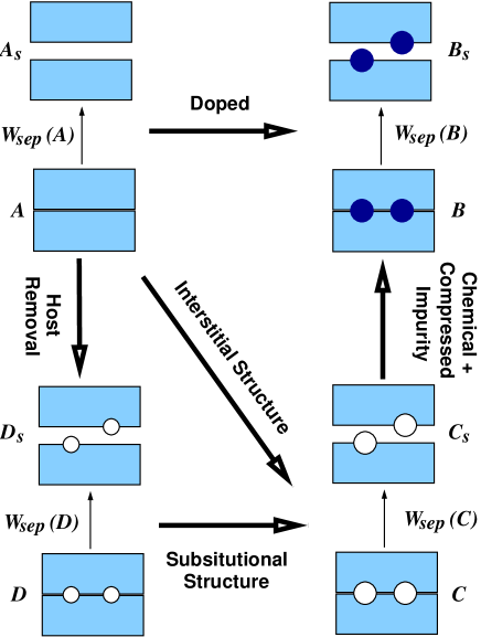
Figure 1: “Ghost impurity cycle” used for discussion of the effect of impurity on grain boundary strength. A and B denote the pure and segregated grain boundaries, respectively, in their equilibrium geometry. Boundary C is created by substituting impurity atoms in B (black spheres) with vacancies (white spheres) without further atomic relaxation. Configuration D is A in which the host atoms that will be replaced by impurity in B  are removed with other atoms kept in place. A_s and B_s denote the free surfaces into which grain boundaries A and B cleave. C_s and D_s are prepared from B_s and C_s  respectively, using the above strategy, namely, impurity atoms in C_s, or host atoms to be replaced by impurity in D_s, are removed keeping the positions of other atoms fixed. Path A$\to$D$\to$C$\to$B refers to substitutional impurities, whereas path A$\to$C$\to$B applies to interstitial impurities (Ref. Lozovoi et al., 2006).

The energy release rate (the minimal energy per unit area of crack advance) associated with brittle cleavage of a grain boundary, $\mathcal{G}_{\mathrm{cleav}}$, is the central quantity characterising the resistance of the boundary to decohesion in the Rice–Thomson–Wang approach.Rice and Thomson (1974); Rice and Wang (1989) If $\mathcal{G}_{\mathrm{cleav}}$ is lower than the energy release rate associated with emitting one dislocation, $\mathcal{G}_{\mathrm{disl}}$, then cracks remain atomically sharp and the crystal breaks in brittle manner. If $\mathcal{G}_{\mathrm{cleav}}>\mathcal{G}_{\mathrm{disl}}$, the crack blunts and the crystal is ductile. Impurity segregation to grain boundaries can either decrease or increase $\mathcal{G}_{\mathrm{cleav}}$. Bi in Cu is a classic example of the former. Copper grain boundaries with bismuth segregating eventually reach the condition $\mathcal{G}_{\mathrm{cleav}}<\mathcal{G}_{\mathrm{disl}}$ leading to a ductile-to-brittle transition.

In the limit of fast separation which we assume in the present study, any impurity exchange between newly formed surfaces and bulk during the decohesion is prevented. In this limit, $\mathcal{G}_{\mathrm{cleav}}$ can be identified with the reversible work of separation

$$\mathcal{G}_{\mathrm{cleav}}=W_{\mathrm{sep}}=\frac{1}{A}\left\{G^{s}-G^{gb}\right\},$$ (1)

where $A$ is the surface area, $G^{gb}$ is the excess Gibbs free energy of a representative piece of material containing grain boundary, and $G^{s}$ is the sum of two excess Gibbs free energies corresponding to surfaces formed after decohesion. Eq. (1) assumes that the impurity excess $\mathit{\Gamma}$ at the grain boundary is equal to the sum of surface impurity excesses. The excess in Eq. (1) is defined with respect to the underlying bulk crystal.

Our ab initio  calculations refer to the zero temperature limit hence the Gibbs free energies are replaced with total energies. It is convenient then to express the changes in $W_{\mathrm{sep}}$ due to impurity in terms of segregation energies per impurity atom, $E_{\mathrm{seg}}$. (Segregation energy is the energy required to remove all impurity from an interface and distribute it in the bulk). Eq. (1) becomes (cf. Eq. (6) in Ref. Lozovoi et al., 2006):

$$W_{\mathrm{sep}}(\mathbf{B})=W_{\mathrm{sep}}(\mathbf{A})+\mathit{\Gamma}\left\{E_{\mathrm{seg}}(\mathbf{B})-E_{\mathrm{seg}}(\mathbf{B}_{\mathbf{s}})\right\}\,,$$ (2)

where A and B denote pure material and material with segregant, respectively. Segregation energies are easy to obtain in an ab initio  supercell approach using the total energies of supercells containing grain boundary (or surface) with and without impurity, $E_{tot}(\mathbf{B})$ and $E_{tot}(\mathbf{A})$, and the same combination for the bulk, $E_{tot}^{b}(\mathbf{B})$ and $E_{tot}^{b}(\mathbf{A})$. For a grain boundary, for example, we have:

$$E_{\mathrm{seg}}(\mathbf{B}) = \frac{1}{N^{gb}}\left\{E_{tot}^{gb}(\mathbf{B})-E_{tot}^{gb}(\mathbf{A})\right\}$$ (3)

$$-\frac{1}{N^{b}}\left\{E_{tot}^{b}(\mathbf{B})-E_{tot}^{b}(\mathbf{A})\right\}\,,$$

where $N^{gb}$ and $N^{b}$ denote the number of impurity atoms included in grain boundary and bulk supercells, respectively. Eq. (3) conveys a simple picture in which an impurity atom at the boundary is exchanged with a host atom in the bulk; if interstitial positions are involved then Eq. (3) should by augmented by adding or subtracting a suitable amount of chemical potentials of the host atoms which, again, are the total energies per atom in pure bulk.

Figure 2: Equilibrium structure of the $\Sigma 5${310}[001] symmetric tilt grain boundary in pure copper. Larger and smaller circles represent alternating (001) Cu planes. The grain boundary plane contains two inequivalent Cu atoms to which we refer as to the “loose” and “tight” sites. The “interstitial” site suitable for segregation of small impurity atoms shown with an asterisk.

Implicit in Eq. (3) is that the bulk is sufficiently dilute so that neither interface nor bulk supercells include any additional randomly distributed impurity atoms. In the dilute limit, the grain boundary impurity excess $\mathit{\Gamma}$ and excess volume $v^{xs}$ per unit area can be found as

$$\mathit{\Gamma} = \frac{N^{gb}}{A}$$ (4)

$$v^{xs} = \frac{1}{A}\left\{V(\mathbf{B})-N^{gb}_{0}\Omega_{0}\right\}\,,$$ (5)

where $V(\mathbf{B})$ is the volume of a relaxed grain boundary supercell with impurity, $N^{gb}_{0}$ is the number of host atoms in this supercell and $\Omega_{0}$ is the atomic volume in pure bulk.

To separate various aspects of grain boundary weakening or strengthening by impurity atoms originating from their size, positions, and chemical identity, the “ghost impurity cycle” introduced in Ref. Lozovoi et al., 2006 and shown in Fig. 1, is rather useful. In this cycle, the direct transition from unsegregated to segregated state A$\to$B is replaced with a gedanken path through intermediate configurations A$\to$D$\to$C$\to$B for both grain boundary and surfaces, and the respective changes in $W_{\mathrm{sep}}$ are evaluated. Configuration C is created from B by removing all impurity atoms without subsequent relaxation. These missing atoms are referred to as “ghosts” since they create forces which keep host atoms in place but do not contribute to the energy of the system in any other way. Such “ghosts” are distorted vacant sites for substitutional impurities or centres of expansion for interstitial impurities. Configuration D is constructed from A in a similar way except that we remove the host atoms defined by impurity sites in B only if these impurities replace host atoms. For interstitial impurities, configuration D is not visited (see interstitial path in Fig. 1).

The same approach is used for the generation of surface configurations A_s–D_s. B_s and A_s represent the equilibrium geometry of free surfaces with and without impurity, respectively. Configuration C_s is created from B_s by removing impurity atoms, whereas in D_s one removes only those host atoms that will be replaced with impurity in B_s. The remaining atoms in C_s and D_s are not allowed to move in response to removal of some of their neighbours. Note that the impurity atoms occupying substitutional positions at a grain boundary can be interstitial impurities at free surfaces (or vice versa). In terms of Fig. 1, this would mean that the substitutional path should be used for grain boundaries, whereas the interstitial path should be taken for surfaces. More generally, one could envisage a situation in which part of impurity atoms occupy interstices whereas the other part substitute host atoms. We shall describe shortly how to deal with such situations.

As argued in Ref. Lozovoi et al., 2006, the change of $W_{\mathrm{sep}}$ at the A$\to$D step describes grain boundary weakening due to some host-host bonds being broken (“host removal” mechanism, HR). Transition D$\to$C corresponds to the distortion of the atomic structure of pure boundary and surface caused by impurity (“substitutional structure” mechanism, SS). Finally, step C$\to$B brings in the impurity-host chemical interactions and, if relevant, associated changes in neighbouring host-host bonds. For oversized impurity atoms, this step also incorporates the elastic energy stored in compressed impurity atoms. These two mechanisms can not be separated hence we refer to this step as “chemical + compressed impurity” mechanism (CC). For more details regarding the cycle and its implementation, the reader is referred to Ref. Lozovoi et al., 2006.

The “ghost impurity cycle” outlined above treats interstitial and substitutional impurities on an equal basis. This is vital for the purposes of the present study in which we shall be introducing boron into substitutional and interstitial positions at a grain boundary, sometimes even simultaneously. The way to deal with the “co-existence” of the substitutional and interstitial paths in Fig. 1 is to formally include configuration D into the latter making it indistinguishable from A. In such case Eq. (2) can be used without making any specific allowances. The same applies to surfaces with impurities occupying adatom positions. These can be treated similarly to interstitial impurities at grain boundaries.

Table 1: Ground-state properties of $\alpha-$B: equilibrium volume, $V_{0}$, rhombohedral lattice constant, $a_{0}$, rhombohedral angle, $\phi$, internal coordinates of boron atoms, $x_{1},z_{1},x_{2},$ and $z_{2}$, bulk modulus, $B$, and the energy difference (per atom) between fcc and $\alpha$ boron, $\Delta E_{fcc}$, obtained in the present study and other ab initio  calculations. Experimental data in the last column are from Ref. Donohue, 1974 unless stated otherwise.

Method	FP LMTO	PAW	PW-PP	LMTO	FP LMTO	PW-PP	PW-PP	PW-PP	PW-PP	US-PP	US-PP	Exp.
LDA or GGA?	LDA		LDA		LDA		LDA	LDA	LDA	GGA	GGA
Reference	present study		Ref. Mailhiot et al.,1990		Ref. Barbee III et al.,1997		Ref. Lee et al.,1990	Ref. Vast et al.,1997	Ref. Masago et al.,2006	Ref. Prasad et al.,2005	Ref. Häussermann et al.,2003	Ref. Donohue,1974
$V_{0}$ (Å3)	6.899	6.993	7.05	6.93	7.06	6.88				6.946	7.30	7.337 [Nelmes et al., 1993]
$a_{0}$ (Å)	4.967	4.989					5.034	4.98	4.967	4.973
$\phi$ (deg.)	58.055	58.063					58.119	58.2	58.65			58.06
$x_{1}$	0.0106	0.0105			0.010							0.0104
$z_{1}$	–0.3460	–0.3458			–0.344							–0.3427
$x_{2}$	0.2211	0.2215			0.220							0.2206
$z_{2}$	–0.3694	–0.3700			–0.369							–0.3677
$B$ (GPa)	232		249	266	230	227			218.4			224 [Nelmes et al., 1993]
$\Delta E_{fcc}$ (eV)	1.30	1.35	1.43	1.83	1.31	1.39

II Calculation details

The $\Sigma 5${310}[001] tilt grain boundary is represented in our study by a periodic supercell containing two grain boundaries with opposite orientation, without any vacuum. Altogether, there are 38 atoms in the supercell, with each atom representing one $\{310\}$ layer, except the grain boundary plain which contains two atoms, the “tight” and the “loose” sites. These two sites together with an “interstitial” site shown in Fig 2, are considered as three possible segregation sites for B. Occupation of any one, any two, or all three of these sites corresponds to 0.5, 1, and 1.5 ML coverage in our notation. As we shall see in Sec. IV.2, severe atomic relaxation of the boundary involving lateral translation of the grains may significantly change the local environment of segregated atoms. We therefore shall be labelling configurations with respect to positions in which the impurity was initially placed.

To represent free (310) surfaces we use the same supercell with 25 layers of copper, the rest being vacuum. Outermost copper layers are replaced with impurity layers if we need to model a segregated surface. The situation in which a grain boundary containing 0.5 or 1.5 ML of impurity cleaves into surfaces with even amount of impurity requires us to double the supercell along the [001] direction. Cubic supercells containing up to 108 atoms (3$\times$3$\times$3 fcc cells) were used to model boron impurities in bulk Cu.

Our first principles calculations employed the full potential LMTO method as implemented in the NFP code.Methfessel et al. (2000) Calculations were semirelativistic, without spin polarisation. We used the local density approximation (LDA) in the parameterisation of von Barth and Hedin, modified by Moruzzi et al.von Barth and Hedin (1972); Moruzzi et al. (1978) Other parameters ($k$-point meshes, real space meshes, etc.) were the same as in Ref. Lozovoi et al., 2006 to which the reader is referred for further details.

III Boron impurity in bulk copper

III.1 Pure boron

Solid boron can exist in a number of relatively stable allotropic modifications—rhombohedral, tetragonal, and even amorphous. It is not clear which phase corresponds to the ground state of B at ambient conditions. Two rhombohedral phases, $\alpha-$ and $\beta-$B are the most likely candidates. $\alpha-$B becomes unstable at 1200${}^{\circ}\mathrm{C}$ and converts to $\beta-$B above 1500${}^{\circ}\mathrm{C}$, but $\beta-$B does not transform back to $\alpha-$B upon cooling (see [Lee et al., 1990] and references therein). Hence kinetic effects must impose severe limitations in this material. $\alpha-$B was found lower in energy by 0.036 eV/atom in Ref. Masago et al., 2006 and by 0.283 eV/atom in Ref. Prasad et al., 2005, and is assumed to represent the ground state in the present study.

The unit cell of the rhombohedral $\alpha-$B consists of twelve atoms forming an icosahedron. Equilibrium structure, bulk modulus and the fcc$-\alpha$ energy difference obtained in our study are in good agreement with other calculations and show the usual discrepancies with experiment associated with the LDA, namely, underestimation of atomic volumes and consequent overestimation of the bulk moduli (see Table 1). Calculations are scalar-relativistic, fully relaxed, and employ the 8$\times$8$\times$8 Monkhorst-Pack mesh of $k$ points. Increasing the $k$ point mesh to 12$\times$12$\times$12 changes the total energy by less than 10^-5 Ry, whereas the forces remain within the convergence criterion 10^-3 Ry/Bohr used throughout the whole study.

Table 2: Boron in bulk Cu: enthalpy of solution $H_{s}$ (per impurity atom) and the relative dilation volume $\Omega_{d}/\Omega_{0}$ of interstitial boron B_i, substitutional boron B_s, and boron dumbells B_d with different orientation. $\Delta H_{s}$ is the enthalpy relative to that of the $s\langle 100\rangle$ dumbell (per entity). $N_{at}$ denotes the number of lattice sites in a supercell used in the calculation, $\Omega_{d}$ is the change of the volume of this supercell when either a single impurity (B_i or B_s) or a dumbell B_d is introduced, $\Omega_{0}$ is the atomic volume in pure fcc Cu, and $E_{a}$ is the activation energy for impurity diffusion. Experimental data on $E_{a}$ are from Ref. Füllgrabe et al., 2001. Theoretical results are obtained by the FP LMTO method unless indicated otherwise.

Impurity	$N_{at}$	$H_{s}$, eV	$\Delta H_{s}$, eV	$\Omega_{d}/\Omega_{0}$	$E_{a}$, eV
Bi	32	1.58	$-$0.10	0.88	1.31
B${}_{i}^{\dagger}$	32	1.63	…	0.93
Bi	108	1.66	0.06	0.89	0.93
Bs	32	1.70	0.02	$-$0.44
Bs	108	1.70	0.10	$-$0.45
Bd:
$a\langle 111\rangle$	32	1.69	1.70	0.52
$s\langle 111\rangle$	32	1.04	0.40	0.38
$a\langle 100\rangle^{\ddagger}$	32	…	…	…
$s\langle 100\rangle$	32	0.84	0	0.25
$s\langle 100\rangle$	108	0.80	0	0.24
Exp.					Bi: 0.57(5)
					Bs: 1.15(10)

^† PAW calculations.
^‡ Unstable, converts to $s\langle 100\rangle$ dumbell during relaxation.

III.2 Copper–boron solid solution

As noted in the Introduction, the available observations do not allow one to conclude unambiguously whether the ground statenot of boron in bulk Cu is interstitial B_i or substitutional B_s. We calculated the heats of solution of the both impurity types using 32 and 108 atom supercells and find that B_i (in octahedral site) is marginally more stable (by 0.04 eV with a 108 atom supercell, Table 2). The difference is small hence it seems reasonable to expect that both B_i and B_s can be found at elevated temperatures, as was indeed observed.Ittermann et al. (1996); Stöckmann et al. (2001); Füllgrabe et al. (2001)

However, as shown in Table 2, either the insertion of a boron atom into an interstice or replacement of a host atom at a regular lattice site both lead to significant volume change, $\Omega_{d}$, negative for B_s and positive for B_i. Hence, one could hypothesise that combining B_s and B_i into a dimer might eliminate most of the elastic distortion of the lattice. To explore this idea, we repeated the calculation with B_i and B_s placed next to each other either along the $\langle 111\rangle$ or $\langle 100\rangle$ directions. In addition, we also considered two boron atoms arranged symmetrically around a vacant site along same directions. We shall refer to the former and the latter as asymmetric and symmetric dumbells, respectively. Among these, the symmetric $\langle 100\rangle$ dumbell, $s\langle 100\rangle$, appears to be the most stable (see Table 2). The heat of solution of the $s\langle 100\rangle$ dumbell is by a factor of two lower than those of the single impurities, indicating that the dumbells should dominate at low temperatures and even survive up to the eutectic temperature $T_{e}=1013$${}^{\circ}\mathrm{C}$.

To verify the last point, we use a simple model in which boron dumbells B_d together with single impurities B_i and B_s are treated as three types of coexisting point defects forming an ideal solution. The model is described in Appendix A, together with the results obtained within this model in the dilute limit. We find in particular, that the concentration of dumbells exceeds those of single impurities in most conditions unless the temperature is close to $T_{e}$ or the boron content is very small. Otherwise, all three impurity forms coexist, both in the single phase and the two phase regions of the Cu–B phase diagram, with the dumbells usually being the dominant kind.

In fact, this can be anticipated already from the difference of the solution enthalpies per entity ($H_{s}$ for single impurities and $2H_{s}$ for dumbells) listed in Table 2 in column $\Delta H_{s}$. These differences serve to estimate the relative amount of defects at terminal solubility (see Eq. (20) in the Appendix).

The fact that adding B to Cu gives rise to three types of competing defects is due to a remarkable coincidence that B atoms are so perfectly “incompatible” with the Cu lattice that the interstitial and substitutional sites are nearly degenerate in energy; and furthermore, boron dumbells stabilised by this misfit strain turn out to have almost the same heat of solution per dumbell as those of the single impurities per atom.

The individual concentrations of the defects might of course change if temperature effects, such as atomic vibrations and lattice expansion, are fully taken into account. In addition, association of several (three, four, etc.) impurities can also play a rôle, at least at low temperatures. Nevertheless, we believe that our results provide a strong indication that in equilibrium copper–boron alloys a significant fraction of the impurities are found in “bound” states.

We are not aware of any metallic system in which dilute impurity would aggregate. Interestingly, Dewing noted that activity measurements of B in molten Cu suggested that B should dimerise in dilute solutions.Dewing (1990) Here we seem to arrive at the same conclusion although for different reasons as elastic strain does not exist in liquids. Our finding might still be relevant to the processing of the experimental data on copper–boron melts as the solid alloy in these studies is customarily assumed to be an idealRexer and Petzow (1970) or regularJacob et al. (2000) solution of fully dissociated impurity atoms.

Another observation that stems from the heats of solution in Table 2 is the fact that the solubility limits indicated in the experimental phase diagram,Massalski (1996) 0.06 at.% at room temperature and 0.29 at.% at $T_{e}$, are much too high in comparison with the enthalpies that we obtained. Assuming that impurity atoms are in the form of dimers and that boron precipitates as the pure rhombohedral $\alpha-$phase, the above solubilities would translate into the Gibbs free energy of solution 0.42 eV/atom at $T_{e}$ and 0.12 eV/atom at room temperature. Assuming single impurities leads to even larger disagreement. Using the aforementioned ideal solution model together with the heats of solution in Table 2 leads to a three orders of magnitude discrepancy in terminal solubility at $T_{e}$, which increases to more than twenty orders of magnitude at room temperature (see Appendix A). Temperature effects can be noticeable at $T_{e}$ but cannot explain the discrepancy at room temperature.

Puzzled with this inconsistency, we compared our FP LMTO calculations with those by the PAW methodBlöchl (1994); Kresse and Joubert (1999) as implemented in the VASP code.Kresse and Hafner (1993); Kresse and Furthmüller (1996) $H_{s}$ obtained for B_i in the 32 atom cell, also shown in Table 2, agrees with the LMTO result within 0.05 eV/atom (the difference almost entirely comes from the energy difference between fcc and $\alpha-$boron obtained by each method, see Table 1). Hence we conclude that the heats of solution presented in Table 2 are the correct LDA result.

The B–Cu phase diagram in Ref. Massalski, 1996 is taken from the critical assessment of available experimental data by Chakrabarti and Laughlin,Chakrabarti and Laughlin (1982) in which the data on maximal solubility of B in Cu are solely based on experimental work by Smiryagin and Kvurt.Smiryagin and Kvurt (1965) The solubility limits mentioned above are those estimated in this latter study (0.05 and 0.01 wt.% B translated into at.%) and appear to serve more as an upper boundary rather than as exact numbers. Chakrabarti and Laughlin indeed comment in their assessment that “it is likely that the actual solubility is even lower than that given by [Smiryagin and Kvurt, 1965].” We expect it to be significantly lower and appeal to future experimental work to correct the terminal boron solubility in published B–Cu phase diagrams.

Table 3: $\Sigma 5$(310)[001] Cu grain boundary with B at various segregation sites: grain boundary excess volume per unit area, $v^{xs}$, average segregation energies per impurity atom, $E_{\mathrm{seg}}$, and the work of separation, $W_{\mathrm{sep}}$. Letters “l”, “t”, and “i” in the second line correspond to impurity atoms being initially placed in the “loose”, “tight”, and “interstitial” positions at the grain boundary plane (see Fig. 2) and then relaxed. The optimal impurity distribution between cleaved surfaces is indicated in the last line. The quantities corresponding to the lowest energy grain boundaries at each coverage are highlighted in bold.

Impurity excess, ML	0	0.5			1			1.5	2
Site		l	t	i	l+t	l+i	t+i	l+t+i
GB excess volume per unit
area $v^{ex}$, Å	0.28	1.02	0.53	0.45	0.87	0.78	0.66	0.98	…
Segregation energy $E_{\mathrm{seg}}$, eV:
to the $(310)$ surface	0	0.40	0.40	0.40	0.17	0.17	0.17	0.37	0.30
to the grain boundary	0	$-$0.66	0.40	0.96	0.51	0.31	0.29	0.46	…
Work of separation $W_{\mathrm{sep}}$, J/m2	3.35	2.49	3.35	3.81	3.57	3.24	3.21	3.58	…
cleavage mode	…	0.5 + 0.5			0.25 + 0.75			0.5 + 0.5	…

IV Boron at a copper grain boundary

IV.1 Work of separation and grain boundary excess volume

The work of separation of a grain boundary at given impurity excess is the difference in total energy between equivalent pieces of material containing the boundary and free surfaces into which the boundary cleaves. Both the grain boundary and the surface pieces should be taken in their lowest energy state.

Figure 3: Convex hull plot for B impurity at Cu(310) surface. Circles correspond to the lowest energy surfaces for each coverage found in our study. 1 ML surface appears to be unstable with respect to decomposition into those with 0.5 and 1.5 ML coverage (dashed line).

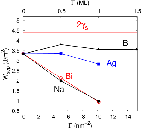
Figure 4: The work of separation of the $\Sigma 5$(310)[001] Cu grain boundary, $W_{\mathrm{sep}}$ as a function of impurity excess $\mathit{\Gamma}$. Data for Bi, Na, and Ag are from Ref. Lozovoi et al., 2006. The horizontal line corresponds to twice the surface energy of Cu(310),Lozovoi et al. (2006) $\gamma_{s}=2.21$ J/m² which provides a natural upper bound for $W_{\mathrm{sep}}$.

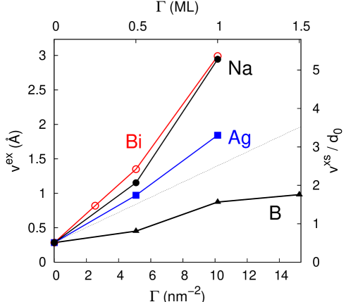
Figure 5: Same as Fig. 4 but for the grain boundary excess volume per unit area, $v^{xs}$. The right hand scale gives $v^{xs}$ in units of {310} interlayer spacing in bulk copper, $d_{0}=0.5576$ Å. The dotted line corresponds to a hypothetical “ideal” impurity identical with Cu atoms.

The lowest energy grain boundary can be found by comparing the energies of relaxed grain boundaries with impurities initially placed into various sites (substitutional or interstitial). This procedure does not, of course, guarantee arrival at the global minimum but is a practical alternative to a full optimisation of grain boundary structure and includes rigid translation of the grains.

The surfaces do not require translations, but a complication here is that one does not know in advance the optimal distribution of the impurity atoms between two newly created surfaces. Usually the impurity splits equally, but not always. More generally, even if equal amount of impurity is experimentally detected for a cleaved macroscopic sample, there still remains a possibility that the surfaces would contain patches with uneven impurity coverage.

The combination of surfaces which produces the lowest energy at given overall amount of impurity can be identified if one employs the convex hull construction. In Fig. 3 we plot the total segregation energy to a surface $G_{\mathrm{seg}}^{s}=\mathit{\Gamma}E_{\mathrm{seg}}^{s}$ as a function of impurity excess $\mathit{\Gamma}$. The quantity $G_{\mathrm{seg}}^{s}$ shows how much the segregation decreases the energy of a piece of material containing a surface. Therefore, any concave region of the curve indicates that there exists a combination of surfaces which provide lower energy. In our case, we find that the 1 ML grain boundary splits into surfaces with coverage 0.5 and 1.5 ML, whereas the other boundaries cleave evenly.

The resulting works of separation are listed in Table 3, together with segregation energies and grain boundary excess volumes. The maximal $W_{\mathrm{sep}}$ for each coverage correspond to the lowest energy grain boundary and are highlighted in bold. We thus find that at 0.5 ML boron prefers the interstitial site and at 1 ML replacing Cu at both the “loose” and “tight” sites provides the best option. Corresponding works of separation are compared with those obtained for Bi, Na, and AgLozovoi et al. (2006) in Fig. 4. Contrary to these latter impurities, boron increases $W_{\mathrm{sep}}$ for the whole range of coverages considered. The largest strengthening effect is observed at 0.5 ML at which $W_{\mathrm{sep}}$ increases by 0.5 J/m²and becomes as large as 3.81 J/m². This can be compared with twice the surface energy of pure Cu,Lozovoi et al. (2006) $2\gamma^{s}_{310}=4.42$ J/m² which provides an upper bound for $W_{\mathrm{sep}}$ above which a grain boundary would become stronger than bulk.

Grain boundary segregation energies in Table 3 compare favourably with experimental estimations of 0.4–0.5 eV,Glikman et al. (1974) especially for high coverages. These energies assume the $s\langle 100\rangle$ dumbells to be the ground state of B in bulk Cu (see Table 2). Had we used interstitial or substitutional B impurities instead, then the segregation energies would have been by 0.8 eV higher. We take this as an independent confirmation of the fact that B impurities in bulk Cu dimerise.

Grain boundary excess volumes $v^{xs}$ in Table 3 are calculated using the dilute bulk limit, Eq. (5). They are smaller than those for Bi, Na, or Ag as shown in Fig. 5. The dotted line in Fig. 5 corresponds to the excess volume if Cu is notionally considered as an impurity (one could think of ⁶⁵Cu isotope, for instance). Segregation of such “ideal” impurity leaves any grain boundary intact, hence, in accord with Eqs. (4)–(5), $v^{xs}(\mathit{\Gamma})$ is a straight line with the slope given by $\Omega_{0}$. The fact, that the excess volumes of grain boundaries with B lie below the dotted line in Fig. 5 indicates a denser packing of atoms at the grain boundary with boron compared to the pure boundary.

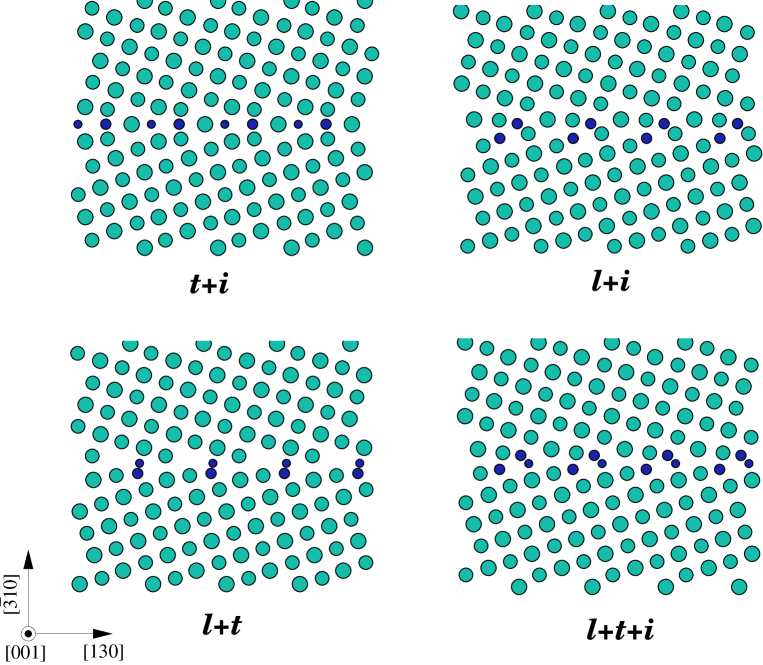
Figure 6: Relaxed $\Sigma 5$ copper grain boundary with 1 and 1.5 ML of boron. For 1.5 ML, boron occupies “loose”, “tight”, and “interstitial” sites at the grain boundary plane. For 1 ML, any two of them are occupied (three combinations). Works of separation and grain boundary excess volumes corresponding to these boundaries are listed in Table 3. Larger and smaller circles correspond to host and impurity atoms lying in neighbouring (001) planes.

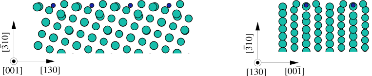
Figure 7: Two side views of the relaxed Cu(310) surface with 0.5 ML of boron. Boron atoms were initially placed instead of the top layer of Cu atoms from which every other atom along the [001] direction was removed. During the relaxation, boron atoms descend below the next Cu layer causing a noticeable distortion of the latter.

IV.2 Atomic structure of the segregated surfaces and grain boundaries

The atomic structure of relaxed grain boundaries with 0.5 ML of boron is relatively simple. The segregated boundaries retain the structure of the equilibrium pure boundary shown in Fig. 2 responding to the insertion of impurity by either minor shrinking (“tight” site) or expansion (“loose” and “interstitial” sites). These boundaries are not shown here.

The structure of grain boundaries with 1 and 1.5 ML are more complex (see Fig. 6). The exception is the “t+i” boundary (i.e. boron atoms segregate to the “tight” and “interstitial” sites) which does not significantly change compared to the pure boundary. However, the average segregation energy of boron to the “t+i” boundary is lower than those for either “t” or “i” 0.5 ML boundaries (see Table 3).

Among the 1 ML boundaries, the lowest energy corresponds to the more open “l+t” boundary in which boron replaces copper at both “loose” and “tight” sites. This boundary experiences a large lateral shift of the grains. As a result of this shift, the boron atoms lying in adjacent (001) planes become nearest neighbours and form boron “strings” running along the [001] direction (normal to the plane of the drawing in Fig. 6).

The “l+i” boundary also entails a rigid translation of the grains. This time, however, boron atoms lie in the same plane and therefore cannot form [001] “strings”. The energy of the “l+i” boundary is close to the energy of the “t+i” boundary despite their atomic structures being very different. As a matter of fact, the “l+i” boundary can be interpreted as the “i” boundary in which the grain boundary plane is shifted normal to itself by one layer and another boron atom substitutes a copper atom in the adjacent plane.

The 1.5 ML “l+t+i” boundary combines the features of the “t+i” boundary (interstitial boron surrounded by six Cu atoms) and the “l+t” boundary (boron “strings”). The average segregation energy for this boundary is close to that of the 1 ML “l+t” boundary.

The following observation is worthwhile here. Substantial fall off of segregation energy with the amount of segregant appears to be a common feature of boron doped intermetallic compounds. As Lejček and Fraczkiewicz note,Lejček and Fraczkiewicz (2003) this could be formally described by either introducing a strong repulsive term into the Fowler–Guggenheim segregation isotherm, or by using the standard Langmuir–McLean isotherm but with limited number of segregation sites. As we observe here, the former approach might be physically misleading, at least for the Cu–B system. For instance, the 1 ML “l+t” boundary containing neighbouring boron atoms is lower in energy than the “t+i” boundary where boron atoms are well separated.

The structure of free (310) surfaces with segregated boron were obtained by replacing copper with boron in the top layer(s) and allowing the surface to relax. For fractional coverages 0.5 and 1.5 ML, we tried either to substitute half of the host atoms in a layer with impurity (substitutional positions) or to place half a monolayer of impurity atoms above the top surface layer (adatom positions). The latter resulted in lower energy configurations.

During relaxation boron atoms embed into the substrate, often going beneath the top copper layer. As a result, the top copper layer becomes strongly distorted. Fig. 7 shows the Cu(310) surface with 0.5 ML of B (and 0.5 ML of vacancies) in the first layer. The plane of B atoms indeed resides below the top layer of Cu atoms and just slightly above the second layer, whereas the host atoms in the surface layer are strongly displaced towards the nearest boron atom.

Table 4: Work of separation $W_{\mathrm{sep}}$ at the vertices of the “ghost impurity cycle” (Fig. 1) and its change $\Delta W_{\mathrm{sep}}$ due to transitions between the vertices. The latter have the meaning of the contributions of the SS, HR, and CC mechanisms. The positive sign of $\Delta W_{\mathrm{sep}}$ corresponds to cohesion enhancement.

Impurity	Site	Excess,	$W_{\mathrm{sep}}$, J/m2					$\Delta W_{\mathrm{sep}}$, J/m2
		ML	A	B	C	D		Total	SS	HR	CC
B	i	0.5	3.35	3.81	3.38	3.35		0.46	0.03	0	0.43
	l	0.5	-”-	2.49	2.20	2.14		$-$0.86	0.06	$-$1.21	0.29
	t	0.5	-”-	3.35	2.87	1.92		0.00	0.95	$-$1.43	0.48
	l+t	1.0	-”-	3.57	3.08	1.35		0.22	1.73	$-$2.00	0.49
	l+i	1.0	-”-	3.24	2.84	2.18		$-$0.11	0.66	$-$1.17	0.40
	t+i	1.0	-”-	3.21	3.15	1.96		$-$0.14	1.19	$-$1.39	0.06
	l+t+i	1.5	-”-	3.58	3.33	1.38		0.23	1.95	$-$1.97	0.25
Bi	l	0.5	-”-	2.15	1.81	2.20		$-$1.20	$-$0.39	$-$1.15	0.34
	l+t	1.0	-”-	0.96	0.13	1.38		$-$2.39	$-$1.25	$-$1.97	0.83

Table 5: Same as Table 4 but for the segregation energies $E_{\mathrm{seg}}$. The latter are average segregations energies per impurity atom (or vacancy). The sign convention is that positive $E_{\mathrm{seg}}$ means that impurity wants to segregate. Segregation energies for the pure boundary $E_{\mathrm{seg}}(\textrm{A})$ are set to zero. The bulk reference used here is an interstitial impurity B_i, not a dumbell B_d as in Table 3.

Impurity	Site	Excess,	$E_{\mathrm{seg}}$, eV							$\Delta E_{\mathrm{seg}}$, eV
		ML	B		C		D			Total		SS		HR		CC
			surf	gb	surf	gb	surf	gb		surf	gb	surf	gb	surf	gb	surf	gb
B	i	0.5	1.18	1.74	$-$0.14	$-$0.10	0	0		1.18	1.74	$-$0.14	$-$0.10	0	0	1.32	1.84
	l	0.5	1.18	0.12	$-$0.14	$-$1.56	0	$-$1.49		1.18	0.12	$-$0.14	$-$0.07	0	$-$1.49	1.32	1.68
	t	0.5	1.18	1.18	$-$0.14	$-$0.73	0	$-$1.76		1.18	1.18	$-$0.14	1.03	0	$-$1.76	1.32	1.91
	l+t	1.0	1.16	1.29	$-$0.34	$-$0.50	$-$0.02	$-$1.25		1.16	1.29	$-$0.32	0.75	$-$0.02	$-$1.25	1.50	1.79
	l+i	1.0	1.16	1.09	$-$0.34	$-$0.65	$-$0.02	$-$0.74		1.16	1.09	$-$0.32	0.09	$-$0.02	$-$0.74	1.50	1.74
	t+i	1.0	1.16	1.07	$-$0.34	$-$0.46	$-$0.02	$-$0.88		1.16	1.07	$-$0.32	0.42	$-$0.02	$-$0.88	1.50	1.53
	l+t+i	1.5	1.15	1.25	$-$0.41	$-$0.42	$-$0.03	$-$0.84		1.15	1.25	$-$0.38	0.42	$-$0.03	$-$0.84	1.56	1.67
Bi	l	0.5	3.11	1.63	1.18	$-$0.71	1.20	$-$0.22		3.11	1.63	$-$0.02	$-$0.49	1.20	$-$0.22	1.93	2.34
	l+t	1.0	3.01	1.54	1.23	$-$0.75	1.22	0.02		3.01	1.54	0.01	$-$0.77	1.22	0.02	1.78	2.29

IV.3 The reasons behind grain boundary strengthening

We now apply the “ghost impurity cycle” to the grain boundaries described in the previous two subsections in order to understand why boron segregation has positive effect on $W_{\mathrm{sep}}$. Contributions from HR, SS, and CC mechanisms defined in Sec. I in terms of the work of separation and segregation energies are listed in Tables 4 and 5, respectively. We choose to evaluate the segregation energies in Table 5 assuming interstitial boron B_i to be the bulk ground state. With this choice, we can directly compare contributions to the SS mechanism with those obtained in other studies, Table 6. The segregation energies for configurations C and D become just energies required to create unrelaxed vacancies at an interface taken with opposite sign (our convention here and in Ref. Lozovoi et al., 2006 is that the bulk impurity is always fully relaxed, whether this is a real impurity or a vacancy; relaxed “interstitial vacancy” is just perfect bulk). If one wants to change to boron dumbells B_d, then the segregation energies in Table 5 should be modified as follows. $E_{\mathrm{seg}}$ for configuration B decreases by 0.78 eV (the difference between the enthalpies of solution of B_i and B_d) and $E_{\mathrm{seg}}$ for configurations C and D decrease by 1.27/2 eV (half the vacancy formation enthalpy in pure bulk, Ref. Lozovoi et al., 2006). Works of separation in Table 4 do not depend on the bulk reference as it cancels out in Eq. (2).

Intuitively, one may expect that segregation of boron to interstitial sites at 0.5 ML coverage would reinforce the boundary because additional atoms lead to additional cohesion across the interface provided that the boundary is not much distorted. Table 4 supports this expectation as the total increase of $W_{\mathrm{sep}}$ by 0.46 J/m² is provided almost exclusively by the CC mechanism. The SS contribution is also positive but small whereas the HR contribution for interstitial impurity is zero by definition. Two other 0.5 ML configurations, “l” and “t”, do not increase $W_{\mathrm{sep}}$ because of the large negative HR contribution arising if boron replaces host atoms.

Table 6: Boron impurity at an interstitial grain boundary site in different materials: contributions of the SS and CC mechanisms in terms of the difference of segregation energies $E_{\mathrm{seg}}^{gb}-E_{\mathrm{seg}}^{s}$ (in eV per impurity atom). For the SS mechanism, individual surface and grain boundary contributions, $E_{\mathrm{seg}}^{s}$ and $E_{\mathrm{seg}}^{gb}$, are also shown. The energies in Refs. [Chen and Wang, 2005; Braithwaite and Rez, 2005; Wu et al., 1996a; Geng et al., 1999; Janisch and Elsässer, 2003] are defined through the difference of binding rather than segregation energies. The results, however, can be compared directly. Note that the SS and CC mechanisms in Refs. [Geng et al., 1999] and [Janisch and Elsässer, 2003] are referred to as the mechanical and chemical contributions, respectively.

Host	Grain boundary	Method	Total	SS			CC	Cohesion	Ref.
			gb – surf	surf	gb	gb – surf	gb – surf	enhancer?
Fe	$\Sigma 5$(010)[001]	DMol (LDA)	1.96	…	…	…	…	yes	[Chen and Wang, 2005]
Fe	$\Sigma 5$(210)[001]	USPP (LDA)	0.49	…	…	…	…	yes	[Braithwaite and Rez, 2005]
Fe	$\Sigma 3$(111)[1$\bar{1}$0]	FLAPW (LDA)	1.07	…	…	…	…	yes	[Wu et al., 1996a]
Ni	$\Sigma 5$(210)[001]	FLAPW (GGA)	0.49	$-$0.27	$-$0.16	0.11	0.38	yes	[Geng et al., 1999]
Mo	$\Sigma 5$(310)[001]	MBPP (LDA)	2.09	$-$0.95	$-$0.23	0.71	1.37	yes	[Janisch and Elsässer, 2003]
Cu	$\Sigma 5$(310)[001]	FP LMTO (LDA)	0.56	$-$0.14	$-$0.10	0.04	0.52	yes	present
									study

A similar effect of interstitial boron is found in ab initio  studies of grain boundaries in Fe, Ni, and Mo (see Table 6). Boron improves the cohesion at all grain boundaries, and this is mostly due to the CC mechanism. The SS contribution enhances grain boundary strength even more despite the surface and grain boundary terms being themselves negative, i.e. boron distorts free surfaces more than grain boundaries.

As boron segregation proceeds beyond 0.5 ML, the boundary is still strengthened although the magnitude of the effect is diminished. Higher coverage configurations necessarily include the removal of host atoms since all interstitial sites are already filled at 0.5 ML. Hence, the mechanism of strengthening is different.

To understand this mechanism, it is instructive to compare boron results with those for bismuth,Lozovoi et al. (2006) reproduced in the Tables for convenience. A striking difference between B and Bi (or other oversized impurities studied in Ref. Lozovoi et al., 2006) is the sign of the SS contribution. The SS mechanism always increases $W_{\mathrm{sep}}$ for boron (Table 4) and decreases $W_{\mathrm{sep}}$ for Bi, Na, and even Ag without any exception. Compare, for example, boron and bismuth at the “loose” site, 0.5 ML coverage. In both cases the boundary is weakened, more by Bi, less by B. The negative HR contributions are similar, the CC mechanism acts so as to strengthen the boundary and is even more efficient for Bi than for B. Thus, it is the SS mechanism which makes the difference, being positive for B but negative for Bi. The “loose” site is not of course the best choice for boron, but even here it is much less harmful than Bi. The comparison of B and Bi for the 1 ML “l+t” case is even more telling. The HR mechanism again, has large detrimental effect for both, the CC mechanism acts in the opposite direction and is nearly twice as large for Bi than for B. Finally, the negative SS contribution is large enough to make the boundary brittle in the Bi case,Lozovoi et al. (2006) but the large and positive SS contribution for B results in the boundary being strengthened. In other words, the difference in the distortion pattern of grain boundaries and surfaces is itself sufficient to either strengthen the boundary or to make it brittle.

What are the reasons for the SS contribution being positive for boron? Let us analyse surface and grain boundary contributions for configurations “l” and “l+t” for B and Bi in Table 5. The surface contribution to the SS mechanism for Bi is negligible, therefore the negative (embrittling) effect comes from the grain boundary distortion. For boron, this differs in two ways. Firstly, there is always a negative surface term, and secondly, the grain boundary term can be large and positive. Even if the latter is negative (as in cases “l” and “i”), it is still smaller than the surface which renders their difference positive.

It is easy to see why the surface contribution to SS is negative for boron. It indicates a sizable distortion of the surface region and arises for impurities that can embed themselves into surface layers (Sec. IV.2). This would be possible for small impurities, especially if they prefer interstitial positions in the bulk.

It is less obvious why the grain boundary contribution to SS tends to be positive. SS contribution in the “ghost impurity cycle” is the energy change when a pure grain boundary with preinserted unrelaxed vacancies D is further deformed as prescribed by “impurity ghosts” to arrive at configuration C. Atoms in configuration D would want to relax towards the vacancies, whereas deformation corresponding to large impurity atoms forces them to move further away. The total energy increases and the SS contribution is negative (embrittling). For small substitutional impurities this is reversed—during the D$\to$C transition atoms move towards the vacancies. Hence, the energy decreases and SS is positive (cohesion enhancing). If boron occupies both interstitial and substitutional sites, atomic displacements are more complex. However, the fact that the grain boundary excess volume is always smaller than that of the “ideal” Cu-like impurity (Fig. 5) indicates that on average the grain boundary shrinks rather than expands.

The above reasoning relies only on the property of boron atoms being “smaller” than host atoms and therefore seems applicable to other undersize impurities, at least for the light metalloid impurities. Boron was found to reinforce grain boundaries in all materials studied (Table 6). Carbon segregation increasesWu et al. (1996b); Janisch and Elsässer (2003) or slightly decreases $W_{\mathrm{sep}}$,Braithwaite and Rez (2005) whereas H, N, and O weaken grain boundaries.Geng et al. (1999); Zhong et al. (2000); Janisch and Elsässer (2003) In the latter case, the embrittling propensity is due to the CC contribution, which becomes large and negative. Janisch and ElsässerJanisch and Elsässer (2003) suggest that this should be the case for light species whose outer electronic shell (1$s$ for H, 2$p$ for N and O) falls near or below the bottom of the valence band of the host metal.

Negative CC indicates that the insertion of an impurity atom into a prepared hole (configuration C) weakens atomic bonds across the interface. This could be the case if the impurity affects the bonds between the neighbouring host atoms by means of withdrawing electronic charge from them—which is known as the electronic mechanism of embrittlement. An alternative explanation, advocated in Ref. Janisch and Elsässer, 2003, is Cottrell’s “unified theory” which refers to the position of the impurity levels relative to the Fermi energy of the host metal.Cottrell (2000) According to this theory, interstitial impurities whose valence electrons lie close to the Fermi level, would form predominantly covalent bonds with host atoms and hence prefer grain boundaries over surfaces due to a higher coordination in the former (the Cottrell $\sqrt{z}$ factor). That means positive CC and cohesion enhancement. On the other hand, impurities with valence states lying high above or deeply below the Fermi level would form polar bonds with the host atoms and turn into screened ions, for which the surface environment is more favourable. This results in a negative CC contribution which weakens the boundary.

In our recent calculations of Cu grain boundary with inert gas atom impurities (He and Kr) we also observed a large negative CC contribution leading to catastrophic embrittlement.Lozovoi and Paxton As no charge transfer to or from inert gas atom is expected, the embrittling effect in this case must be related to the Pauli exclusion principle. One may, therefore, hypothesise that a similar mechanism can act for impurities with nearly completed $p$-shell, such as fluorine, oxygen and, to lesser extent, nitrogen, as filling the impurity shells with metal electrons would effectively render the dopant atoms inert gas like. The question as to how significant this “inert gas atom” mechanism is in comparison with others requires a separate investigation and is outside the scope of the present study.

V Conclusions

The effect of boron impurities at the $\Sigma 5$(310)[001] grain boundary, (310) surface and in the bulk of Cu is investigated on the basis of first principles calculations using the full potential LMTO method.

1. We find that B strengthens the boundary in the whole range of coverages studied (up to 1.5 ML) with the maximal effect achieved at 0.5 ML. Combined with the observed ability of B to remove harmful impurities such as Sb from the copper boundary,Glikman et al. (1974) this makes boron a particularly attractive alloying addition.

2. The reasons behind grain boundary strengthening at 0.5 ML and higher coverages are different. 0.5 ML corresponds to all interstitial positions at the boundary being filled by boron atoms providing therefore additional cohesion between the grains while not distorting the boundary much (the CC mechanism).

3. At 1 and 1.5 ML boron begins to substitute host atoms at the boundary leading to significant distortions and lateral translations of the grains. The SS contribution, however, remains positive and acts so as to increase $W_{\mathrm{sep}}$. We demonstrate that the difference in the sign of the SS contribution proves to be solely responsible for the opposite effect of B compared to embrittling species such as Bi.

4. Distortion of a free surface by segregated boron atoms further increases $W_{\mathrm{sep}}$, but it is not a decisive factor.

5. Introducing boron into bulk Cu leads to a peculiar situation in which substitutional and interstitial impurities are rather close in energy. Combined together, they form a strongly bound dimer held by elastic forces of the host lattice. Remarkably, the heat of solution of the lowest energy $s\langle 100\rangle$ dumbell (per dimer) is also close to the heat of solution of boron single impurities (per atom). Thus a sizable proportion of boron atoms should be found in a bound state in most experimental conditions, even at high temperature.

6. A large discrepancy between calculated heats of solution and experimental estimations for terminal solubility of B in Cu is discovered. We are inclined to think that the solubility limits suggested in Ref. Smiryagin and Kvurt, 1965 and then translated into existing B–Cu phase diagram, are overestimated by a few orders of magnitude and hope that our findings inspire experimental work on the updated version of the phase diagram.

Appendix A Equilibrium concentration of coexisting impurity types in an ideal solution

We describe a thermodynamic approach which we use in the paper to estimate the equilibrium concentration of boron single impurities (B_i and B_s) and dimers (B_d) in bulk Cu. The approach follows the canonical treatment of ideal solid solutions proposed in Ref. Hagen and Finnis, 1998 and is applicable to any binary system in which the heats of solution of the impurity species occupying an interstitial position, a substitutional position, or forming a dumbell, are comparable.

The reader may be surprised by the fact that the model outlined below ignores thermal vacancies altogether. Indeed, at a first glance this looks inconsistent given that the heats of solution of boron in Cu listed in Table 2 are comparable with the vacancy formation enthalpy $H_{f}^{v}=$1.27 eV.Lozovoi et al. (2006) We omit vacancies deliberately as the equilibrium impurity concentrations do not depend on the vacancy formation enthalpy, hence they do not change even if no vacancies at all are allowed. Indeed, if a crystal contains thermal vacancies with concentration $c_{v}$, an additional term will appear in Eqs. (9), (10), and (12), and, consequently, one more relation will be added to the system of equations (13). However, $c_{v}$ can be eliminated from (13) explicitly leading to exactly the same set of equations (14)–(16) as below. The equilibrium impurity concentrations, obtained as the solution of Eqs. (14)–(16), will therefore not depend on the vacancy concentration either. (Note in passing that the reverse is not true, i.e. the equilibrium concentration of vacancies does depend on impurity concentrations.)

A.1 Variables and definitions

Consider a large piece of crystal $A_{1-x}B_{x}$ containing $N$ lattice sites with $n_{a}$ host atoms $A$ and $n_{b}$ impurity atoms $B$. The latter in turn, include $n_{s}$ substitutional impurities, $n_{i}$ interstitial impurities, and $n_{d}$ dumbells:

$$n_{s}+n_{i}+2n_{d}=n_{b}\,.$$

If the crystal is sufficiently large so that any surface effects can be neglected, the resulting equilibrium concentrations should depend on $n_{a}$ and $n_{b}$ only through the composition of the solid solution

$$x=\frac{n_{b}}{n_{a}+n_{b}}\,.$$ (6)

Concentrations of host atoms ($c_{a}$) and impurity of any type ($c_{s},c_{i}$, and $c_{d}$), defined “per lattice site” here, must satisfy the following two constraints:

$$Nc_{a} = n_{a}$$ (7)

$$N\left(c_{s}+c_{i}+2c_{d}\right) = n_{b}\,,$$ (8)

indicating that the total number of atoms of each species is conserved. In addition, we have the “site balance” condition as every lattice position should be occupied by either a host atom, an impurity atom, or an impurity dumbell:

$$c_{a}+c_{s}+c_{d}=1\,.$$ (9)

Overall, there are five variables ($N,c_{a},c_{s},c_{i}$, and $c_{d}$) and three constraints (7)–(9), hence the system has two degrees of freedom.

If defects do not interact, the total energy of the system is linear in defect concentrations:

$$E=N\left(c_{a}\varepsilon_{a}+c_{s}\varepsilon_{s}+c_{i}\varepsilon_{i}+2c_{d}\varepsilon_{d}\right)\,,$$ (10)

where $\varepsilon_{a}$ is the energy (per atom) of the pure crystal, whereas $\varepsilon_{s},\varepsilon_{i},$ and $\varepsilon_{d}$ are the energies per impurity atom defined by Eq. (10). In practice these are usually found from total energy calculation of supercells containing a single defect of each type. Enthalpies of solution $H_{s}$, such as those listed in Table 2, are related to the $\varepsilon$’s in a simple way:

$$H_{s}^{i}=\varepsilon_{i}-\varepsilon_{b};\quad H_{s}^{s}=\varepsilon_{s}-\varepsilon_{b};\quad H_{s}^{d}=\varepsilon_{d}-\varepsilon_{b}\,,$$

where $\varepsilon_{b}$ denotes the energy per atom of species $B$ in its pure state.

At zero pressure, the Gibbs free energy of the crystal is

$$G=E-TS\,,$$ (11)

where $T$ is the temperature and $S$ is the (configurational) entropy given by

$$S = -kN\Big{[}c_{a}\log c_{a}+c_{s}\log c_{s}+c_{d}\log c_{d}-c_{d}\log\eta$$ (12)

$$+ c_{i}\log c_{i}+\left(\alpha-c_{i}\right)\log\left(\alpha-c_{i}\right)-\alpha\log\alpha\Big{]}\,,$$

where $k$ is the Boltzmann constant, $\eta$ is the number of equivalent orientations of the dumbell, and $\alpha$ is the number of interstitial sites per one lattice site. For the octahedral interstices in the fcc lattice $\alpha=1$, whereas $\eta=3$ for the $\langle 100\rangle$ dumbell in cubic crystals. Eqs. (10) and (12) do not take into account atomic vibrations, but these can be easily included, for example, at the level of quasi harmonic approximation.Lozovoi and Mishin (2003)

A.2 Equilibrium concentrations

The equilibrium impurity concentrations are those that minimise the Gibbs free energy (11) subject to constraints (7)–(9). The minimisation leads to the following system of five equations

$$G-\mu_{a}n_{a}-\mu_{b}n_{b} = 0$$

$$\varepsilon_{a}+kT(1+\log c_{a})-\mu_{a}-\lambda/N = 0$$

$$\varepsilon_{s}+kT(1+\log c_{s})-\mu_{b}-\lambda/N = 0$$ (13)

$$2\varepsilon_{d}+kT(1+\log c_{d}/\eta)-2\mu_{b}-\lambda/N = 0$$

$$\varepsilon_{i}+kT\log\left[c_{i}/(\alpha-c_{i})\right]-\mu_{b} = 0\,,$$

where $\mu_{a}$ and $\mu_{b}$ are Lagrange multipliers associated with Eqs. (7) and (8) and therefore have the meaning of the chemical potentials of species $A$ and $B$, respectively. $\lambda$ is the Lagrange coefficient corresponding to Eq. (9). Eqs. (13) together with constraints (7)–(9) are sufficient to determine all the unknowns.

Elimination of $\mu_{a}$, $\mu_{b}$, and $\lambda$ leaves the following two independent relations containing only the impurity concentrations:

$$\frac{c_{i}/\alpha}{(1-c_{i}/\alpha)^{\alpha+1}c_{s}} = \exp\left[-\,\frac{(\varepsilon_{i}-\varepsilon_{s})}{kT}\right]$$ (14)

$$\frac{(c_{i}/\alpha)c_{s}}{(1-c_{i}/\alpha)c_{d}/\eta} = \exp\left[-\,\frac{(\varepsilon_{i}+\varepsilon_{s}-2\varepsilon_{d})}{kT}\right]\,,$$ (15)

in which the reader might immediately recognise “quasi chemical” relations describing defect reactions. Eq. (14), in particular, corresponds to the conversion of a substitutional impurity into an interstitial one, whereas Eq. (15) describes the dissociation of a dumbell into an interstitial and a substitutional impurity.

Eqs. (14)–(15) together with the relation

$$c_{s}+(1-x)c_{i}+(2-x)c_{d}=x$$ (16)

can be used to find all three concentrations $c_{s},c_{i}$, and $c_{d}$. [Eq. (16) readily follows from constraints (7)–(9) and the definition of $x$ (6)].

The above consideration applies to an ideal solid solution of arbitrary composition $x$. If the alloy is dilute, $x\ll 1$, finding the solution of Eqs. (14)–(16) simplifies and reduces to solving the quadratic

$$\left[2\eta\,e_{di}^{2}-e_{si}-\alpha(\alpha+2)\right]z^{2}+\left(e_{si}+\alpha+2x\right)z-x=0\,,$$ (17)

where $e_{di}$ and $e_{si}$ denote the following exponentials

$$e_{di} = \exp\left(-\frac{\varepsilon_{d}-\varepsilon_{i}}{kT}\right)=\exp\left(-\frac{H_{s}^{d}-H_{s}^{i}}{kT}\right)$$

$$e_{si} = \exp\left(-\frac{\varepsilon_{s}-\varepsilon_{i}}{kT}\right)=\exp\left(-\frac{H_{s}^{s}-H_{s}^{i}}{kT}\right)\,.$$

Equilibrium concentrations are then obtained using the positive root of (17), $z_{+}$, as:

$$c_{d}=\eta\,e_{di}^{2}\,z_{+}^{2}\,;\qquad c_{i}=\alpha\,z_{+}\,;\qquad c_{s}=e_{sd}\,z_{+}$$ (18)

A.3 Solubility limit

As pointed out in [Hagen and Finnis, 1998], the advantage of the above approach is that it produces not only the equilibrium concentrations of defects but also the chemical potentials of the species. The chemical potential of the solute, in particular, can be restored from the equilibrium concentrations $c_{d},c_{i}$, and $c_{s}$ using any of the following equations:

$$\mu_{b} = \varepsilon_{s}+kT\left[\log c_{s}+\alpha\log(1-c_{i}/\alpha)\right]$$

$$= \varepsilon_{i}+kT\log\left[c_{i}/(\alpha-c_{i})\right]$$

$$= \varepsilon_{d}+\frac{1}{2}kT\left[\log c_{d}/\eta+\alpha\log(1-c_{i}/\alpha)\right]\,.$$

These three relations simply express the fact that impurity atoms participating in any of the three types of defects considered here, namely interstitial impurity, substitutional impurity, and impurity dumbells, are in equilibrium with each other, hence their chemical potentials must be equal.

Once the chemical potentials are known, it is straightforward to find the limiting solubilities by considering the equilibrium between the $A$-rich and the $B$-rich phases with terminal compositions. The terminal compositions are those that make $\mu_{a}$ and $\mu_{b}$ in the both phases equal.

For our purposes, however, it is sufficient to assume that the $B$-rich phase is a pure $B$ crystal, such as the rhombohedral $\alpha$-boron, with $\mu_{b}=e_{b}$. Using again the dilute limit, from (A.3) we obtain the maximal defect concentrations in $A_{1-x}B_{x}$ as

$$c_{s}^{m} = \exp\left(-\,\frac{H_{s}^{s}}{kT}\right)$$

$$c_{i}^{m} = \alpha\exp\left(-\,\frac{H_{s}^{i}}{kT}\right)$$ (20)

$$c_{d}^{m} = \eta\exp\left(-\,\frac{2H_{s}^{d}}{kT}\right)\,.$$

These, according to (16), define the limiting solubility $x^{m}$ as

$$x^{m}=c_{s}^{m}+c_{i}^{m}+2c_{d}^{m}\,.$$ (21)

Figure 8: Equilibrium concentration of B_d, B_i and B_s in Cu_1-xB_x at T = 1000 K given by Eqs. (17)-(18) as a function of boron content $x$. The vertical dotted line corresponds to the solubility limit $x^{m}$ estimated according to Eq. (21).

Figure 9: Equilibrium concentration of B_d, B_i and B_s and the total amount of boron, $x=c_{i}+c_{s}+2c_{d}$, as a function of $T^{-1}$ (the Arrhenius plot). The alloy composition is taken as the terminal solution at $T=1000$ K (vertical dotted line in Fig. 8). The kink on the curves corresponds to the precipitation of the second phase (assumed to be pure $\alpha-$B). The vertical dotted line indicates the eutectic temperature $T_{e}=1013$${}^{\circ}\mathrm{C}$.

A.4 Results for boron in copper

Fig. 8 shows the equilibrium concentrations of B_i, B_s, and B_d at $T=1000$K as a function of the boron content $x$. These were obtained using Eqs. (17) and (18) with $\alpha=1,\eta=3$, and the enthalpies of solution $H_{s}$ listed in Table 2 (those calculated in a 108 atom supercell). The limiting solubility $x^{m}$ given by Eqs. (20)–(21) is shown with a vertical dotted line.

According to Fig. 8, the dumbells strongly prevail at and above $x^{m}$. (Supersaturated solutions may arise if the excess boron precipitates as some metastable phase, higher in energy than the rhombohedral $\alpha$-B. Such a scenario, however, is not supported by experimental observationsRexer and Petzow (1970)). With $x$ decreasing, the loss of configurational entropy should eventually overweigh the energetic advantage of forming dumbells, giving rise to the crossover between concentration of dumbells and single impurities. This is indeed observed in Fig. 8, although the crossover concentrations seem too small to be experimentally detectable.

Fig. 9 shows the temperature dependence of the impurity concentrations at fixed $x$ in the form of the Arrhenius plot $\log c=f(1/T)$. Concentration $x$ for this plot is chosen as the limiting solubility in Fig. 8. As a result, the curves in Fig. 9 have a kink at $T=1000$ K which corresponds to the precipitation of the second phase. The curves to the left of the kink are the equilibrium defect concentrations in a single phase crystal Cu_1-xB_x given by (17)–(18), whereas concentrations to the right of the kink correspond to a two–phase equilibrium between Cu_1-xB_x and pure $\alpha$-boron. The latter are given by Eq. (20) and are just straight lines in the Arrhenius coordinates.

We again observe the dominance of boron dumbells in the whole range of temperatures, except the narrow region close to the eutectic temperature $T_{e}=1013$${}^{\circ}\mathrm{C}$ (vertical dotted line in Fig. 9). The crossover point appears here for the same reason as in Figs. 8 and rapidly moves to higher temperatures with $x$ increasing. If, for example, for this plot we use $x$ corresponding to the limiting solubility at $T_{e}$, then the crossover would move above both the eutectic temperature and melting temperature of pure copper $T_{m}=1085$${}^{\circ}\mathrm{C}$, so the dumbells would dominate everywhere.

To summarise, we observe that boron dumbells B_d are the essential component of Cu_1-xB_x solid solutions both in the single phase and two phase regions of the Cu–B phase diagram. As a matter of fact, the concentration of boron dumbells B_d exceeds those of single impurities B_i and B_s in most conditions. High temperature and small boron content tend to make these concentrations comparable at best. The dumbells can be suppressed only in very diluted samples where the impurity concentrations are likely to fall below the detection limit anyway.

The terminal solubility of B in Cu appears to be lower than that indicated in published phase diagrams.Massalski (1996) It is of the order of a few ppm at $T_{e}$ (cf. 0.29 at.% in [Massalski, 1996]), and is as low as $10^{-29}$ at room temperature (cf. 0.06 at.% in [Massalski, 1996]). The fact that the second phase precipitates as a solid solution of Cu in BRexer and Petzow (1970); Massalski (1996) rather than as the pure boron (assumed here) should lead to even lower limiting solubilities.

References

- Liu et al. (1985) C. T. Liu, C. L. White, and J. A. Horton, Acta Metall. 33, 213 (1985).
- Lejček and Fraczkiewicz (2003) P. Lejček and A. Fraczkiewicz, Intermetallics 11, 1053 (2003).
- Massalski (1996) T. B. Massalski, ed., Binary Alloy Phase Diagrams (ASM International, Materials Park, Ohio, 1996), 2nd ed.
- Glikman et al. (1974) E. E. Glikman, Y. V. Goryunov, and A. M. Zherdev, Russian Physics Journal 17, 946 (1974).
- Suryanarayanan et al. (1999) R. Suryanarayanan, C. A. Frey, S. M. L. Sastry, B. E. Waller, S. E. Bates, and W. E. Buhro, Mater. Sci. Engng. A 264, 210 (1999).
- Ellis et al. (1999) D. E. Ellis, K. C. Mundim, D. Fuks, S. Dorfman, and A. Berner, Philos. Mag. B 79, 1615 (1999).
- Füllgrabe et al. (2001) M. Füllgrabe, B. Ittermann, H.-J. Stöckmann, F. Kroll, D. Peters, and H. Ackermann, Phys. Rev. B 64, 224302 (2001).
- Lozovoi et al. (2006) A. Y. Lozovoi, A. T. Paxton, and M. W. Finnis, Phys. Rev. B 74, 155416 (2006).
- Rice and Thomson (1974) J. R. Rice and R. Thomson, Phil. Mag. 29, 73 (1974).
- Rice and Wang (1989) J. R. Rice and J.-S. Wang, Mat. Sci. Eng. A107, 23 (1989).
- Donohue (1974) J. Donohue, The Structures of The Elements (Wiley, New York, 1974).
- Mailhiot et al. (1990) C. Mailhiot, J. B. Grant, and A. K. McMahan, Phys. Rev. B 42, 9033 (1990).
- Barbee III et al. (1997) T. W. Barbee III, A. K. McMahan, J. E. Klepeis, and M. van Schilfgaarde, Phys. Rev. B 56, 5148 (1997).
- Lee et al. (1990) S. Lee, D. M. Bylander, and L. Kleinman, Phys. Rev. B 42, 1316 (1990).
- Vast et al. (1997) N. Vast, S. Baroni, G. Zerah, J. M. Besson, A. Polian, M. Grimsditch, and J. C. Chervin, Phys. Rev. Lett. 78, 693 (1997).
- Masago et al. (2006) A. Masago, K. Shirai, and H. Katayama-Yoshida, Phys. Rev. B 73, 104102 (2006).
- Prasad et al. (2005) D. L. V. K. Prasad, M. M. Balakrishnarajan, and E. D. Jemmis, Phys. Rev. B 72, 195102 (2005).
- Häussermann et al. (2003) U. Häussermann, S. I. Simak, R. Ahuja, and B. Johansson, Phys. Rev. Lett. 90, 065701 (2003).
- Nelmes et al. (1993) R. J. Nelmes, J. S. Loveday, D. R. Allan, J. M. Besson, G. Hamel, P. Grima, and S. Hull, Phys. Rev. B 47, 7668 (1993).
- Methfessel et al. (2000) M. Methfessel, M. van Schilfgaarde, and R. A. Casali, in Electronic Structure and Physical Properties of Solids: The Uses of the LMTO Method. Lecture Notes in Physics, 535, edited by H. Dreysse (Springer-Verlag, Berlin, 2000), pp. 114–147.
- von Barth and Hedin (1972) U. von Barth and L. Hedin, J. Phys. C 5, 1629 (1972).
- Moruzzi et al. (1978) V. L. Moruzzi, J. F. Janak, and A. R. Williams, Calculated Electronic Properties of Metals (Pergamon, New York, 1978).
- (23) By the impurity ground state we understand the dominant type of impurity (interstitial, substitutional, etc.) in the single phase alloy in the limit.
- Ittermann et al. (1996) B. Ittermann, H. Ackermann, H.-J. Stöckmann, K.-H. Ergezinger, M. Heemeier, F. Kroll, F. Mai, K. Marbach, D. Peters, and G. Sulzer, Phys. Rev. Lett. 77, 4784 (1996).
- Stöckmann et al. (2001) H.-J. Stöckmann, K.-H. Ergezinger, M. Füllgrabe, B. Ittermann, F. Kroll, and D. Peters, Phys. Rev. B 64, 224301 (2001).
- Dewing (1990) E. W. Dewing, Metall. Trans. A 21, 2609 (1990).
- Rexer and Petzow (1970) J. Rexer and G. Petzow, Metall. 151, 1083 (1970).
- Jacob et al. (2000) K. T. Jacob, S. Priya, and Y. Waseda, Metall. Trans. A 31, 2674 (2000).
- Blöchl (1994) P. E. Blöchl, Phys. Rev. B 50, 17953 (1994).
- Kresse and Joubert (1999) G. Kresse and D. Joubert, Phys. Rev. B 59, 1758 (1999).
- Kresse and Hafner (1993) G. Kresse and J. Hafner, Phys. Rev. B 47, 558 (1993).
- Kresse and Furthmüller (1996) G. Kresse and J. Furthmüller, Phys. Rev. B 54, 11169 (1996).
- Chakrabarti and Laughlin (1982) D. J. Chakrabarti and D. E. Laughlin, Bull. Alloy Phase Diagrams 3, 45 (1982).
- Smiryagin and Kvurt (1965) A. P. Smiryagin and O. S. Kvurt, Tr. Gos. Nauchn. Issled. Proektn. Inst. Splavov Obrabotki Tsvetn. Metal. 24, 7 (1965).
- Chen and Wang (2005) Z.-Z. Chen and C.-Y. Wang, J. Phys.: Condens. Matter 17, 6645 (2005).
- Braithwaite and Rez (2005) J. S. Braithwaite and P. Rez, Acta Mater. 53, 2715 (2005).
- Wu et al. (1996a) R. Wu, L. P. Zhong, L. J. Chen, and A. J. Freeman, Phys. Rev. B 54, 7084 (1996a).
- Geng et al. (1999) W. T. Geng, A. J. Freeman, R. Wu, C. B. Geller, and J. E. Raynolds, Phys. Rev. B 60, 7149 (1999).
- Janisch and Elsässer (2003) R. Janisch and C. Elsässer, Phys. Rev. B 67, 224101 (2003).
- Wu et al. (1996b) R. Wu, A. J. Freeman, and G. B. Olson, Phys. Rev. B 53, 7504 (1996b).
- Zhong et al. (2000) L. Zhong, R. Wu, A. J. Freeman, and G. B. Olson, Phys. Rev. B 62, 13938 (2000).
- Cottrell (2000) A. H. Cottrell, Mater. Sci. Technol. 6, 807 (2000).
- (43) A. Y. Lozovoi and A. T. Paxton, unpublished.
- Hagen and Finnis (1998) M. Hagen and M. Finnis, Phil. Mag. A 77, 447 (1998).
- Lozovoi and Mishin (2003) A. Y. Lozovoi and Y. Mishin, Phys. Rev. B 68, 184113 (2003).