Effect of Leptonic CP Phase in $\nu_{\mu}\to\nu_{\mu}$ Oscillations

Abstract:

In the case of large 1-3 mixing angle as $\sin^{2}2\theta_{13}\geq 0.03$, we investigate the possibility for measuring the leptonic CP phase by using only $\nu_{\mu}\to\nu_{\mu}$ oscillations independently of $\nu_{\mu}\to\nu_{e}$ oscillations. As the result, we find that the best setup to measure the CP phase without strongly depending on the uncertainties of the other parameters is around the energy $E=0.43$GeV and the baseline length $L=5000$km. In this region, the CP phase effect remains even after averaging over the neutrino energy. We also find that there is a CP sensitivity even in the short baseline length $L\leq 1000$km if $\Delta m_{31}^{2}$ is determined with an uncertainty of about $0.1\%$. In the T2KK experiment, we explore the possibility for measuring the CP phase by using a baseline from Tokai to Kamioka after determining $\Delta m_{31}^{2}$ at the baseline to Korea. As the result, we find that some information of the CP phase can be obtained from the measurements.

1 Introduction

The finite mass of neutrinos and the mixings among different flavors have been confirmed in various neutrino experiments. Recently, the LSND anomaly [1] is refused by the result of MiniBOONE experiment [2] and the results obtained in the past neutrino experiments can be almost explained by the neutrino oscillations among three generations. The effect of such neutrino oscillations has been considered not only in the experiments on the earth but also in the far universe for example supernova explosions [3, 4, 5].

For the values of mass squared differences and mixing angles, the results of atmospheric neutrino experiments [6], K2K experiment [7] and MINOS experiment [8] provide

$$|\Delta m^{2}_{31}|\sim 2.5\times 10^{-3}{\rm eV}^{2},\quad\sin^{2}2\theta_{23}\sim 1$$ (1)

and the results of solar neutrino experiments [9] and KamLAND experiment [10] provide

$$\Delta m^{2}_{21}\sim 8.1\times 10^{-5}{\rm eV}^{2},\quad\sin^{2}\theta_{12}\sim 0.31.$$ (2)

On the other hand, only the upper bound for the 1-3 mixing angle

$$\sin^{2}2\theta_{13}\leq 0.16$$ (3)

is obtained from the CHOOZ experiment [11]. We cannot determine the sign of $\Delta m^{2}_{31}$ at present from the experimental data. Furthermore, we have no information on the leptonic CP phase $\delta$. Unveiling these unknown parameters is one of the most important aims in the next generation neutrino experiments. In particular, the value of $\delta$ is very important at the view point of the leptogenesis [12].

One of the serious obstacles in determining the value of $\delta$ is the eight-fold degeneracies [13, 14, 15]. There are some cases in which the uncertainty of $\delta$ becomes large due to the effect of degeneracy. One of the turning points is whether $\theta_{13}$ can be determined by the next generation reactor experiments like Double CHOOZ experiment [16] and the superbeam experiments like T2K experiment [17], NO$\nu$A experiment [18]. In this paper, we concentrate on the cases that $\sin^{2}2\theta_{13}$ is larger than $0.03$ and assume that $\theta_{13}$ will be found in the Double CHOOZ experiment without being affected by the $\theta$-$\delta$ ambiguity. In this case, it is suggested by many authors that the remaining four-fold degeneracies can be also solved within a few decades. One possibility is the observation of neutrinos from the same beam to two detectors on different baselines like Tokai-to-Kamioka-Korea (T2KK) proposal [19] and SuperNO$\nu$A proposal [20]. The other possibilities are the combination of more than two kinds of neutrino sources, long baseline plus atmospheric neutrinos [21, 22] and long baseline plus reactor neutrinos [23]. The possibility for using the Wide Band Beam and analyzing the spectral information of neutrino events is also investigated in ref. [24]. In these proposals, the measurement of the leptonic CP phase is also explored by using $\nu_{\mu}\to\nu_{e}$ ($\nu_{e}\to\nu_{\mu}$) oscillations.

In our previous work [25], we suggested that we can measure the leptonic CP phase by using only $\nu_{\mu}\to\nu_{\mu}$ oscillations in the region $E\leq 2$GeV, $L\geq 2000$km if $\sin^{2}2\theta_{13}$ is large. In the analysis, the probability for $\nu_{\mu}\to\nu_{\mu}$ oscillations can change about $0.4$ by the CP phase effect and then there remains a difference of about $0.2$ between the maximal and minimal values of the probabilities even after averaging over the neutrino energy. In these considerations, we have explored new possibilities of experiments to be performed after a decade in addition to solving parameter degeneracies and determining the value of the CP phase. It is easy to observe the $\nu_{\mu}\to\nu_{\mu}$ oscillations in superbeam experiments and neutrino factory experiments. There is a potential to measure the CP phase $\delta$ independently of $\nu_{\mu}\to\nu_{e}$ oscillations in the case that the parameters except for $\delta$ can be measured precisely. If we assume the unitarity in three generations, the channel of $\nu_{\mu}\to\nu_{e}$ oscillations should be related to that of $\nu_{\mu}\to\nu_{\mu}$ oscillations. This means that we can predict the behavior of one oscillation channel by the behavior of the other channel. (See references [26] about the discussion of the unitarity in the lepton sector, for example.) If we find the difference between this prediction and the experimental result, we must consider effect of new physics and we will have some constraints to the unified theory in the high energy physics. Thus, the measurements of $\delta$ in two independent channels are very important for exploring the new physics beyond the Standard model. Recently, the exact formulation of neutrino oscillation probabilities has been extended to the case of non-standard interaction in view of the era of precision measurement of parameters [27]. A lot of investigations have been also performed about the exploration of non-standard interaction and the non-unitary effect by future experiments. See [28], [29] and the references therein.

In this paper, we give the detailed analysis for the possibility of the measurement of the CP phase in $\nu_{\mu}\to\nu_{\mu}$ oscillations, considering the systematic error, uncertainties of parameters except for $\delta$ and the uncertainty of matter density, which were not considered in our previous work [25]. We investigate the best conditions of baseline length and energy for measuring the CP phase in $\nu_{\mu}\to\nu_{\mu}$ oscillations by using both analytical and numerical methods. We also calculate the baseline dependence and $\theta_{13}$ dependence of CP sensitivity. Furthermore, we consider the reason why we have no CP sensitivity in comparatively short baseline length and show how the CP sensitivity depends on the uncertainty of $\Delta m_{31}^{2}$. We estimate how this uncertainty can be improved in future experiments and how CP sensitivity can become good in comparatively short baseline experiments. We usually use the $\nu_{\mu}\to\nu_{\mu}$ channel in order to measure $\Delta m_{31}^{2}$ precisely. Namely, we need two different baselines to measure the CP phase in the case of short baseline by using this channel. So, we consider the T2KK experiment as concrete setup. We use one baseline from Tokai to Korea to measure the value of $\Delta m_{31}^{2}$ as precise as possible and use another baseline from Tokai to Kamioka to measure the CP phase.

Outline of this paper is the following. In section 2, we explore the energy and the baseline length where the CP dependence in $\nu_{\mu}\to\nu_{\mu}$ oscillations becomes large. In section 3, we assume the concrete experimental setup and calculate the CP sensitivity. In section 4, we clarify what is the problem for measuring the CP phase in relatively short baseline. Then, in section 5, we reinvestigate the CP sensitivity in the case that this problem can be improved. In section 6, we conclude. Finally, in appendix, the approximate formula for the coefficient of $\cos\delta$ is derived, which is applicable for the case of large $L/E$.

2 Region with Large CP Dependence

In this section, let us review the CP dependence of neutrino oscillation probabilities observed in the superbeam experiments. We also investigate the energy and baseline length where the CP dependence becomes large.

The Hamiltonian in matter is represented as

$$H=O_{23}\Gamma H^{\prime}\Gamma^{\dagger}O_{23}^{T},$$ (4)

where $O_{23}$ is the rotation matrix between the second and the third generations and $\Gamma$ is the phase matrix defined by $\Gamma={\rm diag}(1,1,e^{i\delta})$. Without loss of generality, we can factor out the part of $\theta_{23}$ and $\delta$. This makes it possible to include the matter effect only in the reduced Hamiltonian $H^{\prime}$ as

$$H^{\prime}=O_{13}O_{12}{\rm diag}(0,\Delta_{21},\Delta_{31})O_{12}^{T}O_{13}^{T}+{\rm diag}(a,0,0).$$ (5)

Due to this factorization, we can transparently understand how oscillation probabilities depend on the CP phase $\delta$. In the above expression, we use the equalities $\Delta_{ij}=\Delta m_{ij}^{2}/(2E)=(m_{i}^{2}-m_{j}^{2})/(2E)$, $a=\sqrt{2}G_{F}N_{e}\simeq 7.56\times 10^{-5}\cdot\rho Y_{e}$, $G_{F}$ is the Fermi constant, $N_{e}$ is the electron number density, $\rho$ is the matter density, $Y_{e}$ is the fraction of electrons, $E$ is the neutrino energy and $m_{i}$ is the mass of $\nu_{i}$. The CP dependences of the probabilities for $\nu_{\mu}\to\nu_{e}$ oscillation, $\nu_{\mu}\to\nu_{\mu}$ oscillation and $\nu_{\mu}\to\nu_{\tau}$ oscillation are given by

$$P_{\mu e} = A_{\mu e}\cos\delta+B_{\mu e}\sin\delta+C_{\mu e},$$ (6)

$$P_{\mu\mu} \simeq A_{\mu\mu}\cos\delta\hskip 48.36958pt+C_{\mu\mu},$$ (7)

$$P_{\mu\tau} \simeq \hskip 48.36958ptB_{\mu\tau}\sin\delta+C_{\mu\tau},$$ (8)

in ref. [30]. Eqs. (7) and (8) hold exactly in the case of $\theta_{23}=45^{\circ}$ [31], where the coefficients $A_{\mu\alpha}$, $B_{\mu\alpha}$ and $C_{\mu\alpha}$ $(\alpha=e,\mu,\tau)$ are the quantities determined by the parameters except for $\delta$. If we assume the unitarity in the framework of three generations, the sum of these probabilities has to be one for any value of $\delta$. This leads to the relations among the coefficients

$$A_{\mu e}+A_{\mu\mu}\simeq 0,$$ (9)

$$B_{\mu e}+B_{\mu\tau}=0,$$ (10)

$$C_{\mu e}+C_{\mu\mu}+C_{\mu\tau}=1.$$ (11)

It is well known that the order of magnitude for the coefficients is represented as

$$A_{\mu\mu}=-A_{\mu e}=O(\alpha s_{13}),\qquad B_{\mu\tau}=-A_{\mu e}=O(\alpha s_{13}),$$ (12)

$$C_{\mu e}=O(\alpha^{2})+O(s_{13}^{2}),\qquad C_{\mu\mu}=O(1),\qquad C_{\mu\tau}=O(1),$$ (13)

by using the small parameters $\alpha=\Delta_{21}/\Delta_{31}$ and $\sin\theta_{13}=s_{13}$. See ref. [31] for example. It should be noted that the magnitude of $A_{\mu\mu}$ is as same as that of $A_{\mu e}$ and is not so small. Therefore, $\nu_{\mu}\to\nu_{\mu}$ oscillation will be one of the important channels in order to obtain the information on the CP phase, although it is hard to observe the CP phase compared to $\nu_{\mu}\to\nu_{e}$ channel because of the large CP independent term $C_{\mu\mu}$. If we observe some differences between the values of the CP phase measured by the two independent channels, this means the violation of the unitarity in three generations and we can obtain some of the important clues for new physics.

Below, it is considered how we should choose the energy and the baseline in order to measure the CP phase by using only $\nu_{\mu}\to\nu_{\mu}$ oscillations. At first, we numerically calculate the region in $E$-$L$ plane with large $|A_{\mu\mu}|$, which is the coefficient of $\cos\delta$. In this calculation, we use the following parameters, $\Delta m^{2}_{31}=2.5\times 10^{-3}{\rm eV}^{2}$, $\sin^{2}2\theta_{23}=1$, $\Delta m^{2}_{21}=8.1\times 10^{-5}{\rm eV}^{2}$, $\sin^{2}\theta_{12}=0.31$, $\sin^{2}2\theta_{13}=0.16$, $\rho=3.3$g/cm³ and $Y_{e}=0.494$.

In figure 1, the black color shows the region with large $|A_{\mu\mu}|$, namely at relatively low energy $E\leq 2$GeV and a long baseline $L\geq 2000$km. In other words, $|A_{\mu\mu}|$ becomes large in the region with approximately $L({\rm km})/E({\rm GeV})\geq 2000$. However, in present experiments, only the event rate averaging over the energy can be observed in the region with such large $L/E$ due to the finite energy resolution of the detector. Hence, we need to learn whether the CP phase effect remains in such situation and we would like to investigate the condition under which the CP phase effect becomes the largest after averaging.

In order to investigate the behavior of $A_{\mu\mu}$ more accurately, we derived the approximate formula of $A_{\mu\mu}$ from the exact one [32] in the Appendix. In the derivation, we kept in mind that our approximation should be valid for the energy region $E\simeq 0.1$-$10$GeV realized in superbeam experiments. More concretely, we defined $\lambda_{i}$ as the effective mass of $i$-th neutrino divided by $(2E)$ and we took the approximation $\lambda_{1}<\lambda_{2}\ll\lambda_{3}$, $a\ll\lambda_{3}$ and $s_{13}^{2}\ll 1$. Then, we have left only leading order terms of small quantities, $\Delta_{21}$, $\lambda_{1}$, $\lambda_{2}$ and $s_{13}$. In order to be a good approximation for the region with large $L/E$, we did not neglect the term with the order of $O(\Delta_{21}^{\prime})$ included in the oscillating part and multiplied by $L/E$.

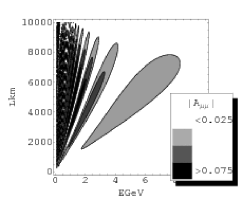
Figure 1: Region with large $|A_{\mu\mu}|$. In the black region, the magnitude of $|A_{\mu\mu}|$ becomes large.

Hence, the approximate formula for $A_{\mu\mu}$ is calculated as

$$A_{\mu\mu} \simeq \underbrace{\frac{4J_{r}\Delta_{21}(a-\Delta_{21}\cos 2\theta_{12})}{\tilde{\Delta}_{21}^{2}}\sin^{2}\tilde{\Delta}_{21}^{\prime}}_{\displaystyle{A_{1}}}\underbrace{-\frac{4J_{r}\Delta_{21}}{\tilde{\Delta}_{21}}\sin\tilde{\Delta}_{21}^{\prime}\sin(2\tilde{\Delta}_{31}^{\prime}-\tilde{\Delta}_{21}^{\prime})}_{\displaystyle{A_{2}}},$$ (14)

where $J_{r}=s_{12}c_{12}s_{23}c_{23}s_{13}c_{13}^{2}$, $\tilde{\Delta}_{ij}=\lambda_{i}-\lambda_{j}$, $\tilde{\Delta}_{ij}^{\prime}=\tilde{\Delta}_{ij}L/2$ and

$$\lambda_{1} \simeq \frac{\Delta_{21}+a-\sqrt{(a-\Delta_{21}\cos 2\theta_{12})^{2}+\Delta_{21}^{2}\sin^{2}2\theta_{12}}}{2}$$ (15)

$$\lambda_{2} \simeq \frac{\Delta_{21}+a+\sqrt{(a-\Delta_{21}\cos 2\theta_{12})^{2}+\Delta_{21}^{2}\sin^{2}2\theta_{12}}}{2}$$ (16)

$$\lambda_{3} \simeq \Delta_{31}.$$ (17)

In eq.(14), $A_{\mu\mu}$ is represented as the sum of two terms $A_{1}$ and $A_{2}$. $A_{1}$ is slowly oscillating term according to the change of energy as controlled by $\tilde{\Delta}_{21}^{\prime}$. $A_{2}$ is rapidly oscillating term as controlled by $\tilde{\Delta}_{31}^{\prime}$. In the small $L/E$ region, $A_{1}$ can be neglected and the main contribution comes from $A_{2}$. As the value of $L/E$ increases, $A_{1}$ also gives the contribution and $A_{2}$ oscillates faster. Therefore, only $A_{1}$ remains in the region with sufficiently large $L/E$ and after averaging over the energy. The total behavior of $A_{\mu\mu}$ can be described as the oscillation around the average value determined by $A_{1}$. The coefficient of sine function in $A_{1}$ is given by

$$\frac{4J_{r}\Delta_{21}(a-\Delta_{21}\cos 2\theta_{12})}{\tilde{\Delta}_{21}^{2}}=\frac{4J_{r}\Delta m^{2}_{21}(2aE-\Delta m^{2}_{21}\cos 2\theta_{12})}{(2aE-\Delta m^{2}_{21}\cos 2\theta_{12})^{2}+\Delta m_{21}^{4}\sin^{2}2\theta_{12}}.$$ (18)

If we use the parameters $\sin^{2}2\theta_{23}=1$ and $\sin^{2}\theta_{12}=0.31$, it is found that the value of local maximum is given by

$$A_{1}^{\rm max}=\frac{2J_{r}}{\sin 2\theta_{12}}\sin^{2}\left(\frac{\sqrt{2}\Delta m^{2}_{21}\sin 2\theta_{12}L}{4E_{\ell}}\right)=\frac{\sin 2\theta_{13}}{4}\sin^{2}\left(\frac{\sqrt{2}\Delta m^{2}_{21}\sin 2\theta_{12}L}{4E_{\ell}}\right)$$ (19)

at the energy

$$E_{\ell}=\frac{\Delta m^{2}_{21}(\cos 2\theta_{12}+\sin 2\theta_{12})}{2a}=0.43{\rm GeV}\cdot\frac{\Delta m^{2}_{21}}{8.1\times 10^{-5}{\rm eV}^{2}}\cdot\frac{3.3{\rm g/cm}^{3}}{\rho}.$$ (20)

If we fix the energy at this value and from the maximal condition $\sqrt{2}\Delta m^{2}_{21}\sin 2\theta_{12}L/4E_{\ell}=(2n+1)\pi/2$ $(n=0,1,2,\cdots)$ for (19), we can determine the baseline length $L_{\ell}$ as

$$L_{\ell}=\frac{\sqrt{2}E_{\ell}(2n+1)\pi}{\Delta m^{2}_{21}\sin 2\theta_{12}}=5000{\rm km}\cdot(2n+1)\cdot\frac{8.1\times 10^{-5}{\rm eV}^{2}}{\Delta m^{2}_{21}}\cdot\frac{\rho}{3.3{\rm g/cm}^{3}}.$$ (21)

If we use the average density calculated in the PREM [33] corresponding to each baseline, $A_{1}$ becomes maximal at $L_{\ell}=5000$km and $10000$km in the earth mantle. We also find from (21) that $A_{1}^{\rm max}$ attains to about $0.1$ in the case of $\sin^{2}2\theta_{13}=0.16$.

Next, let us consider $A_{2}$. The factor $(4J_{r}\Delta_{21}/\tilde{\Delta}_{21})\sin\tilde{\Delta}_{21}^{\prime}$ included in $A_{2}$ does not change so much compared with $\sin(2\tilde{\Delta}_{31}^{\prime}-\tilde{\Delta}_{21}^{\prime})$ for the change of energy. Namely, we regard

$$\frac{4J_{r}\Delta_{21}}{\tilde{\Delta}_{21}}\sin\tilde{\Delta}_{21}^{\prime}\simeq\frac{2J_{r}\Delta m_{21}^{2}}{aE}\sin(aL)$$ (22)

as the amplitude of $A_{2}$ and roughly speaking, the magnitude decreases inversely proportional to the energy. Next, let us consider the oscillating term related to $\Delta_{31}^{\prime}$. The constructive interference of $A_{1}$ and $A_{2}$ occurs in the case of $\sin(2\tilde{\Delta}_{31}^{\prime}-\tilde{\Delta}_{21}^{\prime})\simeq\sin(2\Delta_{31}-a)^{\prime}\simeq-1$. This leads the maximal condition $(2\Delta m^{2}_{31}-2aE)L/(4E)=(4n-1)\pi/2$. In other words, $A_{\mu\mu}$ becomes maximal near the energy

$$E_{n}({\rm GeV})=\frac{4\cdot 1.27\frac{\Delta m^{2}_{31}}{{\rm eV}^{2}}\frac{L}{\rm km}}{(4n-1)\pi+2\cdot 2\cdot 1.27a\frac{L}{\rm km}}\quad(n=1,2,3,\cdots).$$ (23)

From this expression, it is expected that the peak appears near $E=6.7,2.9,1.8\cdots$ GeV in the baseline $L=5000$km. In the case of small energy, we can approximate as

$$E_{n}({\rm GeV})\simeq\frac{4\cdot 1.27\frac{\Delta m^{2}_{31}}{{\rm eV}^{2}}\frac{L}{\rm km}}{(4n-1)\pi}\quad(n=1,2,3,\cdots),$$ (24)

then the difference between the neighboring peaks is given by

$$\Delta E({\rm GeV})=E_{n}-E_{n+1}\simeq\frac{1.27\frac{\Delta m^{2}_{31}}{{\rm eV}^{2}}\frac{L}{\rm km}}{n^{2}\pi}\simeq\frac{3.0\cdot\frac{\Delta m^{2}_{31}}{2.5\cdot 10^{-3}{\rm eV}^{2}}\frac{L}{5000{\rm km}}}{n^{2}},$$ (25)

at the region satisfying the condition $n\gg 1$. Roughly speaking, we can observe the oscillation in the case that the energy resolution $\sigma_{E}$ is smaller than the difference between the neighboring peaks. For example, the energy resolution is given by $\sigma_{e}=0.085$GeV in the case of Water Cherenkov (WC) detector used in the Super-Kamiokande (SK) experiment. From the above condition $\Delta E>\sigma_{e}$, we obtain the condition $n<6$. This means that we can distinguish up to the fifth peak ($E\simeq 1$GeV) at the baseline length of $L=5000$km. In the energy lower than $E\simeq 1$GeV, we cannot distinguish the different peaks and have to take the average. Namely, the effect of $A_{2}$ can be neglected. In figure 2, left and right figures show the magnitude of $A_{\mu\mu}$ and $P_{\mu\mu}$ as the function of energy at the baseline $L=295$km and $5000$km .

In the left figures, the blue and the red lines represent the magnitudes of $A_{\mu\mu}$ and $A_{1}$. In the right figures, the red and the blue lines are corresponding to the probabilities in the case of $\delta=0^{\circ}$ and $\delta=180^{\circ}$ respectively. One can see that the magnitude of $A_{\mu\mu}$ is small in the case of $L=295$km from the top left figure. On the other hand, the CP phase effect is large in the case of $L=5000$km even after the averaging and the value becomes maximal around $E=0.43$GeV. This coincides with the result obtained by the analytical expression. We also find that the peaks appear in the position calculated by $A_{2}$ as we discussed before. In the middle right figure, we have large CP dependence also in the survival probability.

Next, let us consider the case of inverted hierarchy. We obtain the coefficient of $\cos\delta$ in the case of inverted hierarchy by the replacement $\Delta_{31}\to-\Delta_{31}$ in (14) (exactly speaking, we perform the replacement $\Delta_{31}\to-\Delta_{31}+2\Delta_{21}\cos 2\theta_{12}$). $A_{1}$ does not change in this replacement. Therefore, the total event rates in both hierarchies are almost the same in the low energy region. On the other hand, $A_{\mu\mu}$ of inverted hierarchy becomes slightly smaller in high energy region because of the MSW effect [34] due to the 1-3 mixing. Totally, the CP sensitivity is expected to be small in the case of inverted hierarchy compared with the case of normal hierarchy.

Here, we comment the case of anti-neutrino oscillations. We obtain the probability $P_{\bar{\mu}\bar{\mu}}$ for the anti-neutrino oscillations $\bar{\nu}_{\mu}\to\bar{\nu}_{\mu}$ by the replacement $\delta\to-\delta$ and $a\to-a$ in $P_{\mu\mu}$. As there exist only CP even terms in $P_{\mu\mu}$, we only have to replace $a$ to $-a$. We can obtain the energy $\bar{E}_{\ell}$, where $A_{1}$ is maximal, as

$$\bar{E}_{\ell}=\frac{\Delta m^{2}_{21}(-\cos 2\theta_{12}+\sin 2\theta_{12})}{k}=0.17{\rm GeV}\cdot\frac{\Delta m^{2}_{21}}{8.1\times 10^{-5}{\rm eV}^{2}}\cdot\frac{3.3{\rm g/cm}^{3}}{\rho},$$ (26)

by the same procedure performed in $P_{\mu\mu}$. However, $\bar{E}_{\ell}$ is nearly the production energy of $\mu$ and so it would be hard to observe the CP phase effect for this energy. So, we have to measure the CP phase in higher energy region than $\bar{E}_{\ell}$ for the case of anti-neutrinos. Considering also the smallness of the cross section of anti-neutrino, which is about $1/3$ of that of neutrino, the use of neutrinos has an advantage compared with the use of anti-neutrinos for the measurement of the CP phase through $\nu_{\mu}$ ($\bar{\nu}_{\mu}$) events. In figure 3, we show the energy dependence of $A_{\bar{\mu}\bar{\mu}}$ and $P_{\bar{\mu}\bar{\mu}}$ in the baseline of $L=5000$km in left and right figures. In the left figure, the blue and the red lines represent the value of $A_{\bar{\mu}\bar{\mu}}$ and $A_{1}$. In the right figure, the red and the blue lines correspond to the probabilities in case of $\delta=0^{\circ}$ and $\delta=180^{\circ}$ as same as in figure 2. We can see that the absolute value of $A_{1}$ attains up to $0.1$ around the energy $E=0.1$-$0.2$GeV. We also find that the sign of $A_{\bar{\mu}\bar{\mu}}$ is negative over the entire region. This comes from the denominator of $A_{1}$, which has negative sign for the replacement of $a\to-a$

$A_{\mu\mu}$  $L=295$km  normal	$P_{\mu\mu}$  $L=295$km  normal
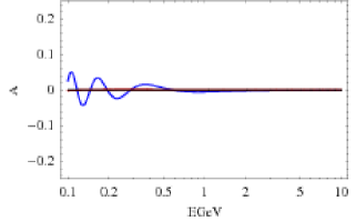
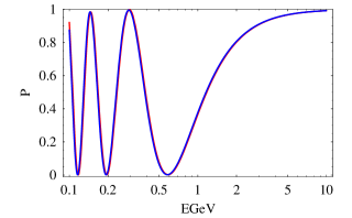
$A_{\mu\mu}$  $L=5000$km  normal	$P_{\mu\mu}$  $L=5000$km  normal
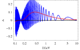
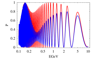
$A_{\mu\mu}$  $L=5000$km  inverted	$P_{\mu\mu}$  $L=5000$km  inverted

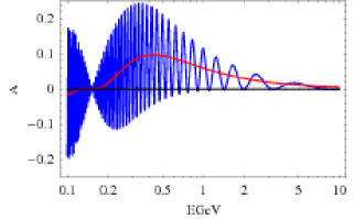
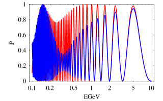
Figure 2: Energy dependence of $A_{\mu\mu}$ and $P_{\mu\mu}$. Left and right figures show the magnitude of $A_{\mu\mu}$ and $P_{\mu\mu}$. In the left figure, blue and red lines represent the magnitudes of $A_{\mu\mu}$ and $A_{1}$ respectively. In the right figure, red and blue lines correspond to the true values of $\delta=0^{\circ}$ and $180^{\circ}$.

$A_{\bar{\mu}\bar{\mu}}$  anti-neutrino	$P_{\bar{\mu}\bar{\mu}}$  anti-neutrino

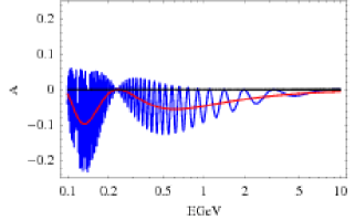
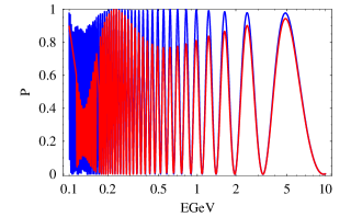
Figure 3: Energy dependence of $A_{\bar{\mu}\bar{\mu}}$ and $P_{\bar{\mu}\bar{\mu}}$. Left and right figures show the magnitude of $A_{\bar{\mu}\bar{\mu}}$ and $P_{\bar{\mu}\bar{\mu}}$. Blue and red lines represent the values of $A_{\bar{\mu}\bar{\mu}}$ and $A_{1}$ respectively in left figure. On the other hand, red and blue lines in right figure represent the probabilities with $\delta=0^{\circ}$ and $180^{\circ}$

Let us summarize the results obtained in this section.

• In $\nu_{\mu}\to\nu_{\mu}$ oscillations, the averaged value of $A_{\mu\mu}$ becomes maximal around the energy $E=0.43$GeV and the baseline length $L=5000$km and $10000$km in the earth mantle.

• The average value of $A_{\mu\mu}$ is positive in the region $E\geq 0.2$GeV. This means that we only have to measure the total rate of $\nu_{\mu}$ events in order to observe the CP phase effect and we need not the good energy resolution of the detector.

• We obtain more information on the CP phase by observing the energy dependence of $\nu_{\mu}$ events at $E\geq 1$GeV in addition to the total rate.

• In relatively short baseline like $L=295$km, the magnitude of $A_{\mu\mu}$ becomes small and the observation of the CP phase effect is difficult unless other parameters except for $\delta$ are precisely known.

• In the case of inverted hierarchy, the CP phase effect included in the total rate is similar to the case of normal hierarchy. The CP dependence in the high energy region is slightly reduced.

• Considering the production energy of $\mu$ and the cross section, it is easy to observe the CP phase in the experiment by neutrinos compared with anti-neutrinos.

• As the CP phase effect is proportional to $s_{13}$, it is difficult to observe in the case of small $s_{13}$.

In the above discussion, we do not consider the decrease of the flux of neutrinos according to the distance. From the statistical point of view, the short baseline is advantageous because of the large event numbers. However, in the case that the ratio of $A_{\mu\mu}$ to the probability is small, the observation of $\delta$ is strongly affected by the uncertainties of other parameters except for $\delta$ as we will discuss later.

3 Estimation of Signal from Leptonic CP Phase

In this section, we estimate how precise the CP phase can be measured in $\nu_{\mu}\to\nu_{\mu}$ oscillations by using $\chi^{2}$ method. As an experimental setup, we consider the 4MW and $2.5^{\circ}$ Off-Axis JPARC beam and WC detector with the fiducial mass of 500kt [17], which is the same as those of T2HK experiment. We take two kinds of baseline length $L=295$km and $5000$km as in the previous section. We assume ten years data acquisition by using only neutrinos. We use the same parameters as in figure 1. We also assume that the mass hierarchy has already been determined before measuring of the CP phase in $\nu_{\mu}\to\nu_{\mu}$ oscillations. For example, the possibility of determining the mass hierarchy by the atmospheric neutrinos was discussed in ref. [21]. They concluded that the observations using the $545$kt WC detector in three years determines the mass hierarchy at 2-$\sigma$ C.L. if $\sin^{2}2\theta_{13}\geq 0.05$. The parameter uncertainties, except for $\delta$, are assumed as 5% for $\theta_{12}$, $\theta_{23}$ and $\theta_{13}$, and as 4% for $\Delta m^{2}_{21}$, and 1% for $\Delta m^{2}_{31}$ by expecting an improvement for the next ten years [35]. We also consider 5% uncertainty of matter density. The energy window for our analysis is $E=0.4$-$1.2$GeV and is divided into 20 bins. We calculate $\Delta\chi^{2}$ by using the energy dependence of QE $\nu_{\mu}$ events and the total rate of CC $\nu_{\mu}$ events. As the backgrounds, we consider NC $\nu_{x}$ events, where $x$ takes all flavors. We set the uncertainties of signal and the background normalization $n_{s}$, $n_{b}$ as $\sigma(n_{s}^{CC})=2.5\%$, $\sigma(n_{s}^{QE})=\infty$, $\sigma(n_{b})=20\%$ and the uncertainties of their tilts $t_{s}$, $t_{b}$ as $\sigma(t_{s})=2\%$, $\sigma(t_{b})=2\%$. As the value of $\sigma(n_{s}^{CC})=2.5\%$ may be optimistic, we discuss how the change of signal normalization affects the results later. The reason for setting $\sigma(n_{s}^{QE})=\infty$ is to be normalization free for QE events and to prevent the double counting in QE and CC events. We use common normalizations and tilts except for this. The expected number of QE events $N_{QEi}$ observed in the i-th bin and CC events $N_{CC}$ are calculated as

$$N_{QEi}=s^{QE}_{i}\left(1+n^{QE}_{s}+t^{QE}_{s}\cdot\frac{E_{i}-\bar{E}}{E_{max}-E_{min}}\right)+b^{QE}_{i}\left(1+n^{QE}_{b}+t^{QE}_{b}\cdot\frac{E_{i}-\bar{E}}{E_{max}-E_{min}}\right),$$ (27)

$$N_{CC}=s^{CC}\left(1+n^{CC}_{s}+t^{CC}_{s}\cdot\frac{E_{i}-\bar{E}}{E_{max}-E_{min}}\right)+b^{CC}\left(1+n^{CC}_{b}+t^{CC}_{b}\cdot\frac{E_{i}-\bar{E}}{E_{max}-E_{min}}\right),$$ (28)

where $s$ and $b$ are the signal and background for the case that the uncertainties of normalization and tilt are not considered. See [36] as the more detail of the definitions. Furthermore, we define $\Delta\chi^{2}$ as

$$\Delta\chi^{2} = \sum_{i=1}^{20}\frac{(N_{QEi}-N_{QEi}^{true})^{2}}{N_{QEi}^{true}}+\frac{(N_{CC}-N_{CC}^{true})^{2}}{N_{CC}^{true}}+\Delta\chi_{sys}^{2}+\Delta\chi_{para}^{2},$$ (29)

$$\Delta\chi_{sys}^{2} = \sum_{\alpha}\left[\left(\frac{n_{s}^{\alpha}}{\sigma(n_{s}^{\alpha})}\right)^{2}+\left(\frac{t_{s}^{\alpha}}{\sigma(t_{s})}\right)^{2}+\left(\frac{n_{b}^{\alpha}}{\sigma(n_{b})}\right)^{2}+\left(\frac{t_{b}^{\alpha}}{\sigma(t_{b})}\right)^{2}\right],$$ (30)

$$\Delta\chi_{para}^{2} = \sum_{i}\left(\frac{X^{i}-X^{i}_{true}}{\sigma(X^{i})}\right)^{2},$$ (31)

by using $N_{QEi}$ and $N_{CC}$, where $\alpha$ in $\Delta\chi^{2}_{sys}$ represents the sum for QE and CC events and $i$ in $\Delta\chi^{2}_{para}$ represents the sum for the parameters. Namely, $X_{i}$ corresponds to the mixing angles, the mass squared differences and the matter density. As the true value of the CP phase, we take $\delta_{true}=90^{\circ}$ and $180^{\circ}$ and plot the value of $\Delta\chi^{2}$ as the function of test value in figure 4. We use the Globes software [37] in this calculation.

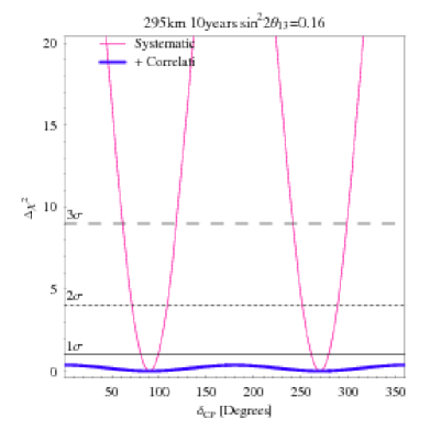
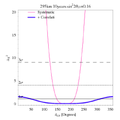
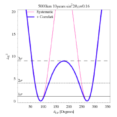
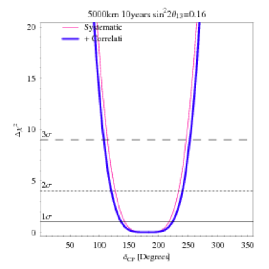
Figure 4: $\Delta\chi^{2}$ by assuming the true values, $\delta_{true}=90^{\circ},180^{\circ}$. The pink line represents $\Delta\chi^{2}$ calculations including only systematics and the blue including also parameter uncertainties. Left and right figures correspond to $\delta_{true}=90^{\circ}$ and $180^{\circ}$. Top and bottom figures are calculated under the assumption of normal hierarchy in the baseline length $L=295$km and $5000$km.

In figure 4, left and right figures correspond to the case of $\delta_{true}=90^{\circ}$ and $180^{\circ}$. Top and bottom figures show the $\Delta\chi^{2}$ calculated in the baseline $L=295$km and $5000$km for the case of normal hierarchy. From the top figures, we can find that the measurement of the CP phase is difficult in $L=295$km because of the uncertainties of parameters. On the other hand, the difficulties are largely decreased for the case of $L=5000$km. We can find from figure 4 that the allowed range is $50^{\circ}$ ($106^{\circ}$) in 1-$\sigma$ (2-$\sigma$) C.L. for $\delta_{true}=90^{\circ}$ and $88^{\circ}$ ($120^{\circ}$) in 1-$\sigma$ (2-$\sigma$) C.L. for $\delta_{true}=180^{\circ}$. We do not show the figures for the case of inverted hierarchy, because they are almost similar to the case of normal hierarchy and only the CP sensitivity becomes slightly worse. This can be understood by using the approximate formula of $A_{\mu\mu}$ given in (14) as follows. Namely, in low energy region, $A_{\mu\mu}$ does not depend on the sign of $\Delta m_{31}^{2}$ because of the averaging of $A_{2}$ and in high energy region, the number of events is suppressed due to the MSW effect compared to the case of normal hierarchy through $A_{2}$.

Next, we investigate how the CP sensitivity depends on the baseline length and the magnitude of $\theta_{13}$. The value of CP sensitivity is shown in figure 5 and figure 6. The CP sensitivity stands for how wide CP angles within $360^{\circ}$ is allowed at certain C.L. when we set a true value of the CP phase. In the case that the allowed range is narrow, we can determine the CP phase precisely. Left and right figures correspond to the case of $\delta_{true}=90^{\circ}$ and $180^{\circ}$. Here, only the case for normal hierarchy is shown as we obtain similar result for inverted hierarchy.

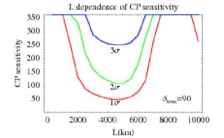
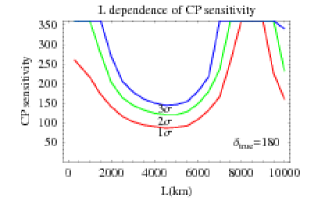
Figure 5: $L$ dependence of CP sensitivity. In left and right figures, we take $\delta_{true}=90^{\circ}$ and $180^{\circ}$. Red, green and blue lines show 1,2 and 3-$\sigma$ C.L. lines respectively. We use the same parameters as in figure 4.

Figure 5 shows the baseline dependence of the CP sensitivity. In the both cases, the best sensitivity is realized around $L=4500\sim 5000$km. This coincides well with the result obtained in (21). In the baseline length of $L=10000$km, the CP sensitivity is not good because of the small statistics due to the too long distance.

Figure 6 shows the $\theta_{13}$ dependence of the CP sensitivity at $L=5000$km. We can see that the CP sensitivity becomes worse gradually according to the decrease of $\theta_{13}$ in both cases. This can be understood by eq.(14) as $A_{\mu\mu}$ is proportional to $s_{13}$. It is also found that the CP sensitivity for $\delta_{true}=180^{\circ}$ is good compared with $\delta_{true}=90^{\circ}$ in 3-$\sigma$ C.L. This is interpreted as follows. In $\nu_{\mu}\to\nu_{\mu}$ oscillations, the probability depends on the CP phase through $\cos\delta$. So, we obtain the largest differences between the probabilities for the two extremes, $\delta=0^{\circ}$ and $\delta=180^{\circ}$, and the probability for $\delta=90^{\circ}$ is in between these two cases. This reduces the difference to other probabilities and the allowed range becomes wide.

Next, let us consider the dependence of CP sensitivity on the systematic errors. As the backgrounds in $\nu_{\mu}$ disapearance channel are small compared to the signal, $\sigma(n_{b})$ and $\sigma(t_{b})$ hardly change the results. The main factor affecting the results is the signal normalization $\sigma(n_{s}^{CC})$.

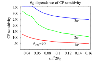
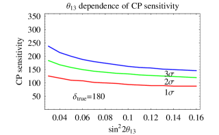
Figure 6: $\theta_{13}$ dependence of CP sensitivity at $L=5000$km. In left and right figures, we take $\delta_{true}=90^{\circ}$ and $180^{\circ}$. Red, green and blue lines show 1,2 and 3-$\sigma$ C.L. lines respectively.

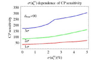
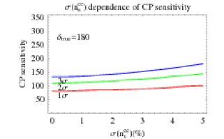
Figure 7: $\sigma(n_{s}^{CC})$ dependence of CP sensitivity at $L=5000$km. In left and right figures, we take $\delta_{true}=90^{\circ}$ and $180^{\circ}$. Red, green and blue lines show 1,2 and 3-$\sigma$ C.L. lines respectively.

Figure 7 shows the dependence of the CP sensitivity on $\nu_{\mu}$ beam normalization at $L=5000$km. We can see that the CP sensitivity becomes worse gradually according to the increase of $\sigma(n_{s}^{CC})$ in both cases. In this baseline, the value of CP phase is mainly determined by the total events averaged over the energy. As the total events are proportional to the $\cos\delta$ through $J_{r}$ in eq.(14), it is considered to be difficult to distinguish the effect of $\delta$ and the signal normalization.

In the end of this section, we consider the reason why the CP sensitivity is so bad for the case of $L=295$km. For the case of the short baseline, we could in principle determine the value of $\delta$ with high accuracy if the parameters, except $\delta$, are precisely determined because of the large statistics. As the flux is inversely proportional to $L^{2}$, the statistics for $L\,=\,295$km becomes about 250 times larger than those for $L\,=\,5000$km. However, the advantage is lost if the other parameters are including a few percent uncertainties. This is due to the small contribution of the CP phase effect to the probability and the CP phase effect is hidden by the large contribution from other parameters. The next question is which parameter prevents the determination of $\delta$. It is found that the uncertainty of $\Delta m_{31}^{2}$ is related to the precise determination of $\delta$ by the numerical calculation as suggested in [38]. In figure 8, we show the dependence of the CP sensitivity at $L=295$km as the function of the uncertainty of $\Delta m_{31}^{2}$ in the case of normal hierarchy. The experimental setup is assumed as the same as that in figure 4. The left and right figures correspond to the cases for $\delta_{true}=90^{\circ}$ and $180^{\circ}$. Horizontal axis represents the $\delta(\Delta m_{31}^{2})/\Delta m_{31}^{2}$ in the unit of %, and the vertical axis represents the value of CP sensitivity. From these figures, it is found that the CP sensitivity becomes gradually good below an uncertainty of $0.6\%$.

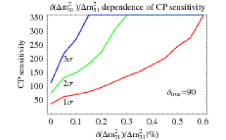
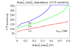
Figure 8: $\delta(\Delta m_{31}^{2})$ dependence of CP sensitivity at $L=295$km. In left and right figures, we take $\delta_{true}=90^{\circ}$ and $180^{\circ}$. Red, green and blue lines show 1,2 and 3-$\sigma$ C.L. lines respectively.

4 Correlation between $\delta$ and the Uncertainty of $\Delta m_{31}^{2}$

In the previous section, it was shown that the uncertainty of $\Delta m_{31}^{2}$ becomes the serious obstacle in determining $\delta$ precisely. In this section, we investigate these correlation in more detail by using the analytical expression and explore the possibility for the improvement.

For the case of $O(\Delta_{21}^{\prime})\ll 1$, the probability $P_{\mu\mu}$ is reduced to the well known expression

$$P_{\mu\mu} \simeq 1-\sin^{2}\Delta_{31}^{\prime}-\frac{8J_{r}\Delta_{21}}{\tilde{\Delta}_{21}}\sin\tilde{\Delta}_{21}^{\prime}\sin\Delta_{31}^{\prime}\cos\Delta_{31}^{\prime}\cos\delta,$$ (32)

as shown in appendix. If we perform the replacements $\Delta_{31}\to\Delta_{31}(1+\epsilon)$ and $\delta\to\delta^{\prime}$, the probability changes as

$$P_{\mu\mu}^{\prime} \simeq 1-\sin^{2}\Delta_{31}^{\prime}-\left(\frac{8J_{r}\Delta_{21}}{\tilde{\Delta}_{21}}\sin\tilde{\Delta}_{21}^{\prime}\cos\delta^{\prime}+\Delta_{31}\epsilon L\right)\sin\Delta_{31}^{\prime}\cos\Delta_{31}^{\prime}$$ (33)

$$= 1-\sin^{2}\Delta_{31}^{\prime}-\frac{8J_{r}\Delta_{21}}{\tilde{\Delta}_{21}}\sin\tilde{\Delta}_{21}^{\prime}\sin\Delta_{31}^{\prime}\cos\Delta_{31}^{\prime}\left(\cos\delta^{\prime}+\frac{\Delta_{31}\epsilon\tilde{\Delta}_{21}L}{8J_{r}\Delta_{21}\sin\tilde{\Delta}_{21}^{\prime}}\right)$$ (34)

up to the leading order of $s_{13}$ and $\epsilon$. Here, we should note that the energy dependence of the correction term from the uncertainty of $\Delta m_{31}^{2}$ is approximately equal to that of the $\cos\delta^{\prime}$ term. Namely, we cannot distinguish two probabilities $P_{\mu\mu}(\Delta_{31}(1+\epsilon),\delta^{\prime})$ and $P_{\mu\mu}(\Delta_{31},\delta)$ when the relation

$$\cos\delta^{\prime}\simeq\cos\delta-\frac{\Delta_{31}\epsilon\tilde{\Delta}_{21}L}{8J_{r}\Delta_{21}\sin\tilde{\Delta}_{21}^{\prime}}\simeq\cos\delta-\frac{\Delta m_{31}^{2}\epsilon aL}{8J_{r}\Delta m_{21}^{2}\sin\frac{aL}{2}}$$ (35)

is satisfied, where we use the approximation $\tilde{\Delta}_{21}\simeq a$. This means that the value of the CP phase cannot be determined if $\epsilon$ is larger than a certain value. This is the correlation between $\delta$ and the uncertainty of $\Delta m_{31}^{2}$ and is a serious obstacle for measuring the CP phase in $\nu_{\mu}\to\nu_{\mu}$ oscillations. The small value of the CP sensitivity in the baseline $L=295$km is due to this correlation.

Next, let us estimate the magnitude of $\epsilon$ giving the small CP sensitivity. If we substitute $a=7.56\cdot 10^{-5}\rho Y_{e}$, $\rho=3.3$g/cm³, $Y_{e}=0.494$, $J_{r}=s_{12}c_{12}s_{23}c_{23}s_{13}c_{13}^{2}\simeq 0.045$, $\Delta m_{31}^{2}=2.5\cdot 10^{-3}$eV² and $\Delta m_{21}^{2}=8.1\cdot 10^{-5}$eV² into (35), we obtain

$$\cos\delta^{\prime}\simeq\cos\delta-\frac{5.3\cdot 10^{-2}\epsilon L}{\sin\left(3.1\cdot 10^{-4}L\right)}.$$ (36)

In the case of relatively short baseline, the above relation is further reduced to

$$\cos\delta^{\prime}\simeq\cos\delta-170\epsilon$$ (37)

and does not depend on the baseline length. Let us illustrate the meaning of this relation in figure 9.

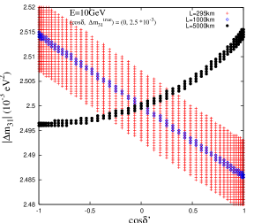
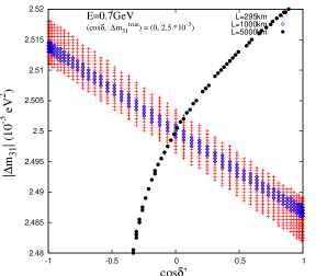
Figure 9: Correlation of $\delta$ with the uncertainty of $\Delta m_{31}^{2}$. In left and right figures, we take $E=10$ GeV and $0.7$ GeV. Regions with same color have almost the same probability given by $|P_{\mu\mu}^{true}-P_{\mu\mu}|<0.001$ $(0.00005)$ in the left (right) figure. Different colors correspond to the different baseline lengths.

In figure 9, regions with same color have almost the same probability as that for $\delta_{true}=90^{\circ}$. More concretely, the region with $|P_{\mu\mu}-P_{\mu\mu}^{true}|\leq 0.001$ $(0.00005)$ is plotted in the left (right) figure. The horizontal axis and vertical axis are taken as $\cos\delta^{\prime}$ and $\Delta m_{31}^{2}$ ($\epsilon$) respectively. Left and right figures represent the case for $E=10$GeV and $0.7$GeV. Red, blue and black colors correspond to the cases for $L=295$km, $1000$km and $5000$km. It is obvious that the value of $\delta$ can be determined by measuring the probabilities for two different energies for the case of $L=5000$km from figure 9, because a superposition of the black curves for the two different energies (left and right figures) would lead to a clear intersection point representing the allowed region. In contrary, we cannot determine the value of $\delta$ for a relatively short baseline like $L=295$km and $1000$km even if the probabilities are measured for two different energies, because of an almost identical overlap of regions with the same color for the two different energies (left and right figures). The overlapping is over the whole range of angles $0^{\circ}\leq\delta\leq 360^{\circ}$. We can determine the slope of these two regions as about $-0.006$, which is almost equal to the coefficient of $\epsilon$, namely $-1/170$ in (37). From this observation, we conclude that the uncertainty of $\Delta m_{31}^{2}$ of more than $0.6\%$ prevents us from determining $\delta$ from $\nu_{\mu}\to\nu_{\mu}$ oscillations only in relatively short baselines. Or in other words, for the case of short baseline length the determination of the CP phase $\delta$ will become possible, if the uncertainty can be decreased below $0.6\%$, as demonstrated in the following section.

5 CP Sensitivity with More Small Uncertainty

In this section, we discuss the possibility for diminishing of parameter uncertainties including $\Delta m_{31}^{2}$ in order to measure $\delta$. We also investigate how the CP sensitivity is improved in a relatively short baseline superbeam experiment after diminishing of parameter uncertainties. It is discussed that the uncertainty of $\Delta m_{21}^{2}$ can be reduced up to $3\%$ at 3-$\sigma$ by loading $0.1\%$ Gd in the detector of SK [39] and that the uncertainty of $\sin^{2}\theta_{12}$ can be reduced up to $2\%$ at 1-$\sigma$ by using the reactor experiment with the baseline of $L\sim 60$km [40]. From these analysis, there is a possibility for diminishing the uncertainties up to $1\%$ at 1-$\sigma$ C.L. for both $\Delta m_{21}^{2}$ and $\theta_{12}$ in near future experiments. The uncertainty of $\Delta m_{31}^{2}$ can be reduced up to $1\%$ at the T2K experiment and the NO$\nu$A experiment. However, it is required that the uncertainty has to be reduced one more order of magnitude in order to receive the sensitivity for the CP phase as discussed in the previous section. So, we consider two baselines. We measure the value of $\Delta m_{31}^{2}$ as precisely as possible in one baseline and then measure the value of $\delta$ by using only $\nu_{\mu}\to\nu_{\mu}$ oscillations in another baseline. As one of the real models, we consider the T2KK experiment [19]. In this experiment, the neutrinos emitted from Tokai are observed in two detectors at Kamioka and Korea. One of the aims in the T2KK experiment is to decrease the systematic error by using the same beam, but we use this experiment to reduce the uncertainty of $\Delta m_{31}^{2}$. Here, we assume that we perform the precise measurement of $\Delta m_{31}^{2}$ in Korea WC detector at $L=1000$km with $500$kt fiducial mass and then we measure the value of $\delta$ in Kamioka WC detector at $L=295$km with the same size. The size of detectors assumed here is larger than those considered in [19].

At first, we set the true value of $\Delta m_{31}^{2}$ as $2.5\cdot 10^{-3}$eV² and calculate $\Delta\chi^{2}$ as the function of test value at $L=1000$km. Here, we consider the case of normal hierarchy. In the case of inverted hierarchy, we obtain the similar features. In our analysis, we consider $\delta$ as free parameter and set the uncertainties of $1\%$ for $\Delta m_{21}^{2}$ and $\theta_{12}$. We use the same uncertainties as in sec.3 for other parameters. Figure 10 shows the value of $\Delta\chi^{2}$. Pink and blue lines correspond to the case of $\delta_{true}=90^{\circ}$ and $180^{\circ}$. We take into account not only the systematic error but also the uncertainties of various parameters in calculating $\Delta\chi^{2}$. From this figure, the test values separated from the true value more than $0.2$-$0.3\%$ can be excluded at 1-$\sigma$ C.L. with 2 d.o.f.

Figure 11 shows the value of $\Delta\chi^{2}$ as the function of test value $\delta$, fixing the uncertainty of $\Delta m_{31}^{2}$ to $0.2\%$ at 1-$\sigma$. About uncertainties of other parameters, we use the same as in figure 10.

We found that there is the CP sensitivity even at relatively short baseline like $L=295$km due to the decrease of parameter uncertainties. For $\delta_{true}=90^{\circ}$, the allowed range is $86^{\circ}$ ($190^{\circ}$) at 1-$\sigma$ (2-$\sigma$) and for $\delta_{true}=180^{\circ}$ the allowed range is $100^{\circ}$ ($148^{\circ}$) at 1-$\sigma$ (2-$\sigma$). In such short baseline, we have an advantage in the statistical point of view. Therefore, this strategy may be better if we can determine the parameters precisely in future experiments.

In figure 12, we show the $\theta_{13}$ dependence of the CP sensitivity in the baseline $L=295$km when $\delta(\Delta m_{31}^{2})/\Delta m_{31}^{2}$ is fixed at $0.2\%$. The experimental setup is the same as in sec.3.

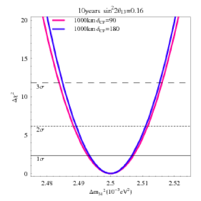
Figure 10: Precision of $\Delta m_{31}^{2}$. Blue and pink lines correspond to the case of $\delta_{true}=90^{\circ}$ and $180^{\circ}$. $\Delta\chi^{2}$ is calculated considering both systematics and parameter uncertainties.

From figure 12, we can see that the CP sensitivity becomes worse mildly according to the decrease of $\theta_{13}$ as in figure 6. In the case of $\delta_{true}=90^{\circ}$ and $180^{\circ}$, the allowed range is about $222^{\circ}$ and $160^{\circ}$ respectively at 1-$\sigma$ for the value of $\sin^{2}2\theta_{13}=0.03$.

Finally, let us comment the dependence of CP sensitivity on the systematic errors. In the baseline of $L=295$km, the first term $A_{1}$ in eq.(14) can be neglected and only the second term $A_{2}$ contributes to the determination of $\delta$. Namely, we obtain the information of $\delta$ by the energy dependence of QE $\nu_{\mu}$ events. In our analysis, we take the signal normalization of QE $\nu_{\mu}$ events as free from the beginning. Therefore, the signal normalization hardly affect the CP sensitivity in this baseline. This is in contrast to the case of $L=5000$km.

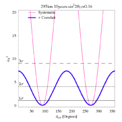
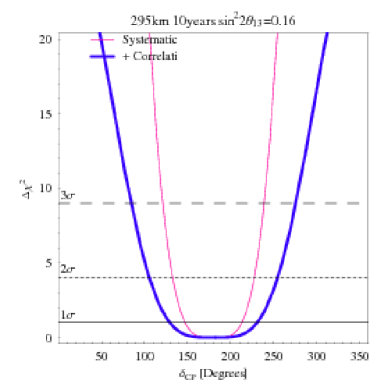
Figure 11: $\Delta\chi^{2}$ by assuming the true values, $\delta=90^{\circ},180^{\circ}$. Pink and blue lines represent the $\Delta\chi^{2}$ considering only systematics and including also parameter uncertainties.

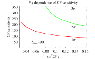
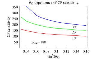
Figure 12: $\theta_{13}$ dependence of CP sensitivity. In left and right figures, we take $\delta_{true}=90^{\circ}$ and $180^{\circ}$. Red, green and blue lines show 1,2 and 3-$\sigma$ C.L. lines respectively.

6 Summary and Discussion

In this paper, we have explored new possibilities for experiments to be performed in the next decade for the case that $\sin^{2}2\theta_{13}$ is larger than $0.03$. The $\theta_{13}$ will be determined in the next generation reactor experiments. Concretely, we have investigated whether the CP phase can be measured by only $\nu_{\mu}\to\nu_{\mu}$ oscillations independently of $\nu_{\mu}\to\nu_{e}$ oscillations. If we can measure the CP phase in two different channels independently and there is a difference for these values, this would be considered as an evidence of new physics. Below, the results obtained in this paper are listed.

• At first, we have investigated the energy and the baseline where the $\cos\delta$ term included in $P_{\mu\mu}$ becomes large by using both numerical and analytical methods. As the result, we found from (20) and (21) that the coefficient $A_{\mu\mu}$ has its largest value around $E=0.43$GeV and $L=5000$ and $10000$km in the earth mantle. The difference of the probabilities attains the maximal value about $0.2$ due to the CP phase effect even after the averaging over the energy.

• Next, we have considered the same beam and the detector as in the T2HK experiment but the baseline $L=295$km and $5000$km and have calculated the CP sensitivity by using $\chi^{2}$ method. As the result, when the uncertainty of $\Delta m_{31}^{2}$ is larger than $1\%$, the CP sensitivity has its best value for the baseline around $L=5000$km. The allowed range becomes $50^{\circ}$ ($88^{\circ}$) at 1-$\sigma$ in $L=5000$km when $\delta_{true}=90^{\circ}$ ($180^{\circ}$). On the other hand, we have almost no sensitivity for the CP phase in the case of $L=295$km because of the effect of parameter uncertainties.

• We have shown both numerically and analytically that the uncertainty of $\Delta m_{31}^{2}$ is particularly important in determining the value of $\delta$. If the uncertainty of $\Delta m_{31}^{2}$ will be less than $0.6\%$, a certain sensitivity for $\delta$ will be obtained even in the relatively short baseline like $L\leq 1000$km.

• We have explored the possibility for measuring the CP phase in relatively short baseline by diminishing the uncertainty of $\Delta m_{31}^{2}$. As concrete experimental setup, we have considered the T2KK experiment. We used one baseline from Tokai to Korea in order to determine $\Delta m_{31}^{2}$ precisely and used the other baseline from Tokai to Kamioka to measure the CP phase by $\nu_{\mu}\to\nu_{\mu}$ oscillations. As the result, the uncertainty of $\Delta m_{31}^{2}$ can be reduced up to about $0.2\%$ and the allowed range becomes about $222^{\circ}$ ($160^{\circ}$) at 1-$\sigma$ when $\delta_{true}=90^{\circ}$ ($180^{\circ}$) at 1-$\sigma$. So, we have the possibility for measuring the CP phase although the sensitivity is not so good.

In future, the mixing angles and the mass squared differences are precisely measured in various kinds of experiments. If $\theta_{13}$ is found in the next generation reactor experiments in addition to this improvement, it will be very important to consider the strategy for exploring the new physics. As one of the strategies, the possibility for measuring the CP phase in $\nu_{\mu}\to\nu_{\mu}$ oscillation is interesting. We will further investigate in our next work how the contribution of new physics appears in future experiments.

Appendix A Derivation of Approximate Formula for $A_{\mu\mu}$

In this appendix, let us derive the approximate formula of $A_{\mu\mu}$ used in sec.2 for the case of constant matter.

At first, in the case of $\theta_{23}=45^{\circ}$ and the symmetric matter profile, the probability is given by

$$P_{\mu\mu}=A_{\mu\mu}\cos\delta+C_{\mu\mu}+D\cos 2\delta,$$ (38)

from the exact formula [30, 32]. Here, we can neglect $D$ because of the higher order terms of small parameters. Concrete expression for $A_{\mu\mu}$ [32] is given by

$$A_{\mu\mu} = \sum_{(ijk)}^{{\rm cyclic}}\frac{8[J_{r}\Delta_{21}\Delta_{31}\lambda_{k}(\lambda_{k}-\Delta_{31})-(A_{\mu\mu})_{k}]}{\tilde{\Delta}_{jk}^{2}\tilde{\Delta}_{ki}^{2}}\cos\tilde{\Delta}_{ij}^{\prime}\sin\tilde{\Delta}_{jk}^{\prime}\sin\tilde{\Delta}_{ki}^{\prime},$$ (39)

where

$$(A_{\mu\mu})_{k} = \Delta_{21}^{2}J_{r}\times\left[\Delta_{31}\lambda_{k}(c_{12}^{2}-s_{12}^{2})+\lambda_{k}^{2}s_{12}^{2}-\Delta_{31}^{2}c_{12}^{2}\right].$$ (40)

In the energy region around $E=1$GeV, we have $\lambda_{1}=O(\Delta_{21}),\lambda_{2}=O(\Delta_{21})$ and $\lambda_{3}\simeq\Delta_{31}$. From these order counting, we can neglect $\lambda_{1}$ and $\lambda_{2}$ compared with $\lambda_{3}$. On the other hand, we cannot neglect $\Delta_{21}^{\prime}$ included in the oscillating term for long baseline such that the relation $\Delta_{21}^{\prime}=\Delta m_{21}^{2}L/4E=O(1)$ is satisfied. If we leave only leading order terms in small parameters $\Delta_{21}$ and $s_{13}$, the expression for $A_{\mu\mu}$ is reduced to

$$A_{\mu\mu} \simeq \frac{8J_{r}\Delta_{21}\Delta_{31}[\lambda_{1}(\lambda_{1}-\Delta_{31})+\Delta_{31}\Delta_{21}c_{12}^{2}]}{\tilde{\Delta}_{31}^{2}\tilde{\Delta}_{21}^{2}}\cos\tilde{\Delta}_{23}^{\prime}\sin\tilde{\Delta}_{31}^{\prime}\sin\tilde{\Delta}_{12}^{\prime}$$

$$+ \frac{8J_{r}\Delta_{21}\Delta_{31}[\lambda_{2}(\lambda_{2}-\Delta_{31})+\Delta_{31}\Delta_{21}c_{12}^{2}]}{\tilde{\Delta}_{32}^{2}\tilde{\Delta}_{21}^{2}}\cos\tilde{\Delta}_{31}^{\prime}\sin\tilde{\Delta}_{12}^{\prime}\sin\tilde{\Delta}_{23}^{\prime}$$

$$= \frac{4J_{r}\Delta_{21}\Delta_{31}[\lambda_{1}(\lambda_{1}-\Delta_{31})+\Delta_{31}\Delta_{21}c_{12}^{2}]}{\tilde{\Delta}_{31}^{2}\tilde{\Delta}_{21}^{2}}\sin\tilde{\Delta}_{12}^{\prime}\{\sin\tilde{\Delta}_{21}^{\prime}+\sin(\tilde{\Delta}_{31}^{\prime}-\tilde{\Delta}_{23}^{\prime})\}$$

$$+ \frac{4J_{r}\Delta_{21}\Delta_{31}[\lambda_{2}(\lambda_{2}-\Delta_{31})+\Delta_{31}\Delta_{21}c_{12}^{2}]}{\tilde{\Delta}_{32}^{2}\tilde{\Delta}_{21}^{2}}\sin\tilde{\Delta}_{12}^{\prime}\{\sin\tilde{\Delta}_{21}^{\prime}-\sin(\tilde{\Delta}_{31}^{\prime}-\tilde{\Delta}_{23}^{\prime})\}$$

$$= -\frac{4J_{r}\Delta_{21}\Delta_{31}}{\tilde{\Delta}_{21}^{2}}\sin\tilde{\Delta}_{21}^{\prime 2}$$

$$\times\left[\frac{\lambda_{1}(\lambda_{1}-\Delta_{31})+\Delta_{31}\Delta_{21}c_{12}^{2}}{\tilde{\Delta}_{31}^{2}}+\frac{\lambda_{2}(\lambda_{2}-\Delta_{31})+\Delta_{31}\Delta_{21}c_{12}^{2}}{\tilde{\Delta}_{32}^{2}}\right]$$

$$+\frac{4J_{r}\Delta_{21}\Delta_{31}}{\tilde{\Delta}_{21}^{2}}\sin\tilde{\Delta}_{12}^{\prime}\sin(2\tilde{\Delta}_{31}^{\prime}-\tilde{\Delta}_{21}^{\prime})$$

$$\times\left[\frac{\lambda_{1}(\lambda_{1}-\Delta_{31})+\Delta_{31}\Delta_{21}c_{12}^{2}}{\tilde{\Delta}_{31}^{2}}-\frac{\lambda_{2}(\lambda_{2}-\Delta_{31})+\Delta_{31}\Delta_{21}c_{12}^{2}}{\tilde{\Delta}_{32}^{2}}\right]$$ (41)

$$\simeq \frac{4J_{r}\Delta_{21}}{\tilde{\Delta}_{21}^{2}}\sin\tilde{\Delta}_{21}^{\prime 2}\left[\lambda_{1}-2\Delta_{21}c_{12}^{2}+\lambda_{2}\right]-\frac{4J_{r}\Delta_{21}}{\tilde{\Delta}_{21}}\sin\tilde{\Delta}_{21}^{\prime}\sin(2\tilde{\Delta}_{31}^{\prime}-\tilde{\Delta}_{21}^{\prime})$$

$$\simeq \frac{4J_{r}\Delta_{21}}{\tilde{\Delta}_{21}^{2}}\sin\tilde{\Delta}_{21}^{\prime 2}\left[a-\Delta_{21}\cos 2\theta_{12}\right]-\frac{4J_{r}\Delta_{21}}{\tilde{\Delta}_{21}}\sin\tilde{\Delta}_{21}^{\prime}\sin(2\Delta_{32}^{\prime}).$$

This is the derivation of (14). In this approximate formula, the MSW effect due to the 1-3 mixing angle is not included, so there is some differences from the exact one in high energy. On the other hand, this approximate formula coincides well in low energy. In this expression, if $L/E$ is small enough, the first term can be neglected and is reduced to

$$A_{\mu\mu}\simeq-\frac{4J_{r}\Delta_{21}}{\tilde{\Delta}_{21}}\sin\tilde{\Delta}_{21}^{\prime}\sin(2\Delta_{32}^{\prime})\simeq-\frac{8J_{r}\Delta_{21}}{\tilde{\Delta}_{21}}\sin\tilde{\Delta}_{21}^{\prime}\sin(\Delta_{31}^{\prime})\cos(\Delta_{31}^{\prime}).$$ (42)

This is the third term of (32).

References

-
[1]
LSND collaboration, A. Aguilar et al.,
Evidence for neutrino oscillations from the observation of
appearance in a beam, Phys. Rev. D64 (2001) 112007
hep-ex/0104049]. - [2] The MiniBooNE Collaboration, A. A. Aguilar-Arevalo et al., A search for electron neutrino appearance at the scale, Phys. Rev. Lett. 98 (2007) 231801 arXiv:0704.1500].
- [3] K. Takahashi, M. Watanabe, K. Sato and T. Totani, Effects of neutrino oscillation on the supernova neutrino spectrum, Phys. Rev. D64 (2001) 093004 hep-ph/0105204].
-
[4]
S. Ando and K. Sato,
A comprehensive study of neutrino spin-flavour conversion in supernovae
and the neutrino mass hierarchy, JCAP 0310 (2003) 001
hep-ph/0309060];
E. K. Akhmedov and T. Fukuyama, Supernova prompt neutronization neutrinos and neutrino magnetic moments, JCAP 0312 (2003) 007 hep-ph/0310119]. - [5] T. Yoshida et al., Supernova neutrino nucleosynthesis of light elements with neutrino oscillations, Phys. Rev. Lett. 96 (2006) 091101 astro-ph/0602195]; Neutrino oscillation effects on supernova light element synthesis, Astrophys. J. 649 (2006) 319 astro-ph/0606042].
-
[6]
Super-Kamiokande Collaboration, Y. Fukuda et al.,
Evidence for oscillation of atmospheric neutrinos, Phys. Rev. Lett. 81
(1998) 1562 hep-ex/9807003];
Super-Kamiokande Collaboration, Y. Ashie et al., A measurement of atmospheric neutrino oscillation parameters by Super-Kamiokande I, Phys. Rev. D71 (2005) 112005 hep-ex/0501064]. - [7] K2K Collaboration, M. H. Ahn et al., Measurement of neutrino oscillation by the K2K experiment, Phys. Rev. D74 (2006) 072003 hep-ex/0606032].
- [8] MINOS Collaboration, D. G. Michael et al., Observation of muon neutrino disappearance with the MINOS detectors and the NuMI neutrino beam, Phys. Rev. Lett. 97 (2006) 191801 hep-ex/0607088].
-
[9]
Super-Kamiokande Collaboration, J. Hosaka et al.,
Solar neutrino measurements in Super-Kamiokande-I, Phys. Rev. D73
(2006) 112001 hep-ex/0508053];
SNO Collaboration, B. Aharmim et al., Electron energy spectra, fluxes, and day-night asymmetries of 8B solar neutrinos from the 391-day salt phase SNO data set, Phys. Rev. C72 (2005) 055502 nucl-ex/0502021]. - [10] KamLAND Collaboration, K. Eguchi et al., First results from KamLAND: evidence for reactor anti-neutrino disappearance, Phys. Rev. Lett. 90 (2003) 021802 hep-ex/0212021]; KamLAND Collaboration, T. Araki et al., Measurement of neutrino oscillation with KamLAND: evidence of spectral distortion, Phys. Rev. Lett. 94 (2005) 081801 hep-ex/0406035].
- [11] CHOOZ Collaboration, M. Apollonio et al., Limits on neutrino oscillations from the CHOOZ experiment, Phys. Lett. B466 (1999) 415 hep-ex/9907037].
- [12] M. Fukugita and T. Yanagida, Baryogenesis without grand unification, Phys. Lett. B174 (1986) 45.
- [13] J. Burguet-Castell, M.B. Gavela, J.J. Gomez-Cadenas, P. Hernandez and O. Mena, On the measurement of leptonic CP violation, Nucl. Phys. B608 (2001) 301 hep-ph/0103258].
- [14] H. Minakata and H. Nunokawa, Exploring neutrino mixing with low energy superbeams, JHEP 0110 (2001) 001 hep-ph/0108085].
- [15] V. Barger, D. Marfatia and K. Whisnant, Breaking eight-fold degeneracies in neutrino CP violation, mixing, and mass hierarchy, Phys. Rev. D65 (2002) 073023 hep-ph/0112119].
- [16] The Double-CHOOZ collaboration, F. Ardellier et al., Letter of intent for Double-CHOOZ: a search for the mixing angle , hep-ex/0405302.
-
[17]
The T2K collaboration, Y. Itow et al.,
The JHF-Kamioka neutrino project,
hep-ex/0106019. - [18] NOvA Collaboration, D. S. Ayres et al., NOvA proposal to build a 30 kiloton off-axis detector to study neutrino oscillations in the Fermilab NuMI beamline, hep-ex/0503053.
-
[19]
M. Ishitsuka, T. Kajita, H. Minakata and H. Nunokawa,
Resolving neutrino mass hierarchy and CP degeneracy by two identical detectors with different baselines,
Phys. Rev. D72 (2005) 033003 hep-ph/0504026];
K. Hagiwara, N. Okamura and K. Senda, Solving the neutrino parameter degeneracy by measuring the T2K off-axis beam in Korea, Phys. Lett. B637 (2006) 266 [Erratum-ibid. B641 (2006) 486] hep-ph/0504061]. - [20] O. Mena Requejo, S. Palomares-Ruiz and S. Pascoli, Super-NOvA: a long-baseline neutrino experiment with two off-axis detectors, Phys. Rev. D72 (2005) 053002 hep-ph/0504015].
- [21] R. Gandhi et al., Mass hierarchy determination via future atmospheric neutrino detectors, Phys. Rev. D76 (2007) 073012 arXiv:0707.1723].
-
[22]
P. Huber, M. Maltoni and T. Schwetz,
Resolving parameter degeneracies in long-baseline experiments by atmospheric neutrino data,
Phys. Rev. D71 (2005) 053006 hep-ph/0501037];
S. T. Petcov and T. Schwetz,
Determining the neutrino mass hierarchy with atmospheric neutrinos,
Nucl. Phys. B740 (2006) 1 hep-ph/0511277];
J. Bernabeu, S. Palomares Ruiz and S.T. Petcov, Atmospheric neutrino oscillations, and neutrino mass hierarchy, Nucl. Phys. B669 (2003) 255 hep-ph/0305152]. -
[23]
K. Hiraide et al.,
Resolving degeneracy by accelerator and reactor neutrino oscillation experiments,
Phys. Rev. D73 (2006) 093008 hep-ph/0601258];
T. Kajita, H. Minakata, S. Nakayama and H. Nunokawa, Resolving eight-fold neutrino parameter degeneracy by two identical detectors with different baselines, Phys. Rev. D75 (2007) 013006 hep-ph/0609286]. - [24] V. Barger et al., Precision physics with a wide band super neutrino beam, Phys. Rev. D74 (2006) 073004 hep-ph/0607177].
- [25] K. Kimura, A. Takamura and T. Yoshikawa, Measuring the leptonic CP phase in oscillations, Phys. Lett. B642 (2006) 372 hep-ph/0605308].
-
[26]
J. Sato, Neutrino oscillation and CP violation,
Nucl. Instrum. Meth. A472 (2000) 434 hep-ph/0008056];
H. Zhang and Z. Z. Xing, Leptonic unitarity triangles in matter, Eur. Phys. J. C41 (2005) 143 hep-ph/0411183];
Y. Farzan and A. Yu. Smirnov, Leptonic unitarity triangle and CP-violation, Phys. Rev. D65 (2002) 113001 hep-ph/0201105]. - [27] O. Yasuda, On the exact formula for neutrino oscillation probability by Kimura, Takamura and Yokomakura, arXiv:0704.1531.
-
[28]
M. Honda, N. Okamura and T. Takeuchi,
Matter effect on neutrino oscillations from the violation of universality in neutrino neutral current interactions,
hep-ph/0603268;
N. Kitazawa, H. Sugiyama and O. Yasuda, Will MINOS see new physics?, hep-ph/0606013;
M. Blennow, T. Ohlsson and J. Skrotzki, Effects of non-standard interactions in the MINOS experiment, hep-ph/0702059;
A. Esteban-Pretel, R. Tomas and J. W. F. Valle, Probing non-standard neutrino interactions with supernova neutrinos, Phys. Rev. D76 (2007) 053001 arXiv:0704.0032];
G.L. Fogli, E. Lisi, A. Marrone, D. Montanino and A. Palazzo, Probing non-standard decoherence effects with solar and KamLAND neutrinos, Phys. Rev. D76 (2007) 033006 arXiv:0704.2568];
N.C. Ribeiro, H. Minakata, H. Nunokawa, S. Uchinami and R. Zukanovich-Funchal, Probing non-standard neutrino interactions with neutrino factories, JHEP 12 (2007) 002 arXiv:0709.1980];
J. Kopp, M. Lindner and T. Ota, Discovery reach for non-standard interactions in a neutrino factory, Phys. Rev. D76 (2007) 013001 hep-ph/0702269]; J. Kopp, M. Lindner, T. Ota and J. Sato, Non-standard neutrino interactions in reactor and superbeam experiments, Phys. Rev. D77 (2008) 013007 arXiv:0708.0152]. -
[29]
S. Antusch, C. Biggio, E. Fernandez-Martinez, M.B. Gavela and J. Lopez-Pavon,
Unitarity of the leptonic mixing matrix,
JHEP 0610 (2006) 084 hep-ph/0607020];
E. Fernandez-Martinez, M.B. Gavela, J. Lopez-Pavon and O. Yasuda, CP-violation from non-unitary leptonic mixing, Phys. Lett. B649 (2007) 427 hep-ph/0703098]. - [30] H. Yokomakura, K. Kimura and A. Takamura, Overall feature of CP dependence for neutrino oscillation probability in arbitrary matter profile, Phys. Lett. B544 (2002) 286 hep-ph/0207174].
-
[31]
A. Takamura, K. Kimura and H. Yokomakura,
Proposal of a simple method to estimate neutrino oscillation probability and CP-violation in matter,
Phys. Lett. B595 (2004) 414 hep-ph/0403150];
Enhancement of CP-violating terms for neutrino oscillation in earth matter,
Phys. Lett. B600 (2004) 91 hep-ph/0407126];
A. Takamura and K. Kimura, Large non-perturbative effects of small and on neutrino oscillation and CP-violation in matter, JHEP 0601 (2006) 053 hep-ph/0506112]. - [32] K. Kimura, A. Takamura and H. Yokomakura, Exact formula of probability and CP-violation for neutrino oscillations in matter, Phys. Lett. B537 (2002) 86 hep-ph/0203099]; Exact formulas and simple CP dependence of neutrino oscillation probabilities in matter with constant density, Phys. Rev. D66 (2002) 073005 hep-ph/0205295]; Analytic formulation of neutrino oscillation probability in constant matter, J. Phys. G29 (2003) 1839.
- [33] A. M. Dziewonski and D. L. Anderson, Preliminary reference Earth model, Phys. Earth Planet. Interiors 25 (1981) 297.
-
[34]
L. Wolfenstein,
Neutrino oscillations in matter, Phys. Rev. D17 (1978) 2369;
S. P. Mikheyev and A. Yu. Smirnov, Resonance enhancement of oscillations in matter and solar neutrino spectroscopy, Yad. Fiz. 42 (1985) 1441 [Sov. J. Nucl. Phys. 42 (1985) 913];
Resonant amplification of neutrino oscillations in matter and solar neutrino spectroscopy, Nuovo Cim. C9 (1986) 17. - [35] T. Schwetz, Neutrino oscillations: current status and prospects, Acta Phys. Polon. B36 (2005) 3203 hep-ph/0510331].
- [36] P. Huber, M. Lindner, W. Winter, Superbeams versus neutrino factories, Nucl. Phys. B645 (2002) 3 hep-ph/0204352].
- [37] P. Huber, M. Lindner and W. Winter, Simulation of long-baseline neutrino oscillation experiments with GLoBES 2005, Comput. Phys. Commun. 167 (2005) 195 hep-ph/0407333].
- [38] A. Donini, E. Fernandez-Martinez, D. Meloni and S. Rigolin, disappearance at the SPL, T2K-I, NOA and the neutrino factory, Nucl. Phys. B743 (2006) 41 hep-ph/0512038].
- [39] S. Choubey and S. T. Petcov, Reactor anti-neutrino oscillations and gadolinium loaded Super-Kamiokande detector, Phys. Lett. B594 (2004) 333 hep-ph/0404103].
- [40] A. Bandyopadhyay, S. Choubey, S. Goswami and S.T. Petcov, High precision measurements of in solar and reactor neutrino experiments, Phys. Rev. D72 (2005) 033013 hep-ph/0410283].