Chiral Odd Generalized Parton Distributions in Impact Parameter Space

Abstract

We investigate the chiral odd generalized parton distributions (GPDs) for the quantum fluctuations of an electron in QED. This provides a field theory inspired model of a relativistic spin $1/2$ composite state with the correct correlation between the different light-front wave functions (LFWFs) in Fock space. We express the GPDs in terms of overlaps of LFWFs and obtain their representation in impact parameter space when the momentum transfer is purely transverse. We show the spin-orbit correlation effect of the two-particle LFWF as well as the correlation between the constituent spin and the transverse spin of the target.

I Introduction

Generalized parton distributions (GPDs) contain a wealth of information about the nucleon structure (see rev for example). At zero skewness $\xi$, if one performs a Fourier transform (FT) of the GPDs with respect to (wrt) the momentum transfer in the transverse direction $\Delta_{\perp}$, one gets the so called impact parameter dependent parton distributions (ipdpdfs), which give how the partons of a given longitudinal momentum are distributed in transverse position (or impact parameter $b_{\perp}$) space. These obey certain positivity constraints and unlike the GPDs themselves, have probabilistic interpretation bur . The $x$ moment of the GPDs give the nucleon form factors. The ipdpdfs were first introduced in the context of the form factors in soper . Ipdpdfs are defined for nucleon states localized in the transverse position space at $R_{\perp}$. In order to avoid a singular normalization constant, one can take a wave packet state. A wave packet state which is transversely polarized is shifted sideways in the impact parameter space burchi . This gives an interesting interpretation of Ji’s angular momentum sum rule ji : the expectation value of the transverse spin operator receives contribution from the second $x$ moment of both the GPDs $H(x,0,0)$ as well as $E(x,0,0)$; the term containing $E(x,0,0)$ arises due to a transverse deformation of the GPDs in the center of momentum frame and the term containing $H(x,0,0)$ arises due to an overall transverse shift when going from transversely polarized nucleons in the instant form to the front form.

At leading twist, there are three forward parton distributions (pdfs), namely, the unpolarized, helicity and transversity distribution. Similarly, three leading twist generalized quark distributions can be defined which in the forward limit, reduce to these three forward pdfs. The third one is chiral odd and is called the generalized transversity distribution $F_{T}$. It is parametrized in terms of four GPDs, namely $H_{T}$, $\tilde{H}_{T}$, $E_{T}$ and $\tilde{E}_{T}$ in the most general way markus ; chiral ; burchi . Unlike $E$, which gives a sideways shift in the unpolarized quark density in a transversely polarized nucleon, the chiral-odd GPDS affect the transversely polarized quark distribution both in unpolarized and in transversely polarized nucleon in various ways. $\tilde{E}_{T}$ does not contribute when skewness $\xi=0$, as it is an odd function of $\xi$. $H_{T}$ reduces to the transversity distribution in the forward limit when the momentum transfer is zero. Unlike the chiral even GPDs, information about which can be and has been obtained from deeply virtual Compton scattering and hard exclusive meson production, it is very difficult to measure the chiral odd GPDs. At present there is only one proposal to get access to them through diffractive double meson production double . There is also a prospect of gaining information about their Mellin moments from lattice QCD. They have been investigated in a constituent quark model in barbara , where a model independent overlap in terms of LFWFs is also given. However, the chiral odd GPDs provide valuable information on the correlation between the spin and angular momentum of quarks inside the proton chiral and so it is worthwhile to investigate their general properties.

The impact representation of GPDs has been extended to the chirally odd sector in chiral . In this work, we investigate the chiral odd GPDs for the quantum fluctuations of a lepton in QED at one-loop order drell , the same system which gives the Schwinger anomalous moment $\alpha/2\pi$. One can generalize this analysis by assigning a mass $M$ to the external electrons and a different mass $m$ to the internal electron lines and a mass $\lambda$ to the internal photon lines with $M<m+\lambda$ for stability. In this work, we use $M=m$ and $\lambda=0$. In effect, we shall represent a spin-${1\over 2}$ system as a composite of a spin-${1\over 2}$ fermion and a spin-$1$ vector boson dis ; dip ; dip2 ; marc ; si . This model has the advantage that it is lorentz invariant, and has the correct correlation between the Fock components of the state as governed by the light-front eigenvalue equation. Also, it gives an intuitive understanding of the spin and orbital angular momentum of a composite relativistic system orbit . In the light-front gauge $A^{+}=0$, the GPDs are expressed as overlaps of the light-front wave functions (LFWFs). Because of Lorentz invariance, $\xi$ dependence of the $x$ moment of the GPDs gets canceled between the $2-2$ and $3-1$ overlaps and one automatically gets the form factors as a function of the momentum transfer squared overlap . We take the skewness to be zero.

The plan of the paper is as follows. In section II we calculate the chiral odd GPDs for a dressed electron state at one loop in QED. In section III we calculate the corresponding ipdpdfs. Conclusions are presented in section IV.

II Chiral odd generalized parton distributions

The chiral odd generalized quark distribution is parametrized as :

$$F^{j}_{T}(x,\xi,t) = -i\int\frac{dy^{-}}{8\pi}\,e^{ixP^{+}\frac{y^{-}}{2}}\,\langle P^{\prime},\sigma^{\prime}|\,\bar{\psi}(-\frac{y^{-}}{2})\sigma^{+j}\gamma_{5}\psi(\frac{y^{-}}{2})|\,P,\sigma\rangle\,$$ (1)

$$= -\frac{i}{2P^{+}}\left[H_{T}(x,\xi,t)\,\bar{u}\sigma^{+j}\gamma_{5}\,u+\tilde{H}_{T}(x,\xi,t)\,\bar{u}\frac{\epsilon^{+j\alpha\beta}\Delta_{\alpha}P_{\beta}}{m^{2}}u\right.$$

$$\left.+E_{T}(x,\xi,t)\,\bar{u}\frac{\epsilon^{+j\alpha\beta}\Delta_{\alpha}\gamma_{\beta}}{2m}u+\tilde{E}_{T}(x,\xi,t)\,\bar{u}\frac{\epsilon^{+j\alpha\beta}P_{\alpha}\gamma_{\beta}}{m}u\,\right].$$

We have omitted the helicity indices of the spinors. Here $j=1,2$ are the transverse components, $u(P)$ and $\bar{u}(P^{\prime})$ are the initial and final state proton spinors respectively. The totally antisymmetric tensor is given by $\epsilon^{+-12}=-2$. We use kinematical variables ${\bar{P}}=(1/2)(P+P^{\prime})$, $\Delta=P^{\prime}-P$, $t=\Delta^{2}=-(\Delta_{\perp})^{2}$. The r.h.s can be calculated using the LF spinors

$$u_{\uparrow}(p)={1\over\sqrt{2p^{+}}}\left(\begin{array}[]{c}p^{+}+m\\ p^{1}+ip^{2}\\ p^{+}-m\\ p^{1}+ip^{2}\end{array}\right)\,,$$ (6)

$$u_{\downarrow}(p)={1\over\sqrt{2p^{+}}}\left(\begin{array}[]{c}-p^{1}+ip^{2}\\ p^{+}+m\\ p^{1}-ip^{2}\\ -p^{+}+m\end{array}\right)\,,$$ (11)

where $m$ is the mass of the fermion. In order to calculate the l. h. s. of the Eq. (1), we use the two-component formalism in two . The ‘good’ light-front (LF) components of the fermion field are projected by $\psi^{\pm}=\Lambda^{\pm}\psi$ with $\Lambda^{\pm}={\frac{1}{2}}\gamma^{0}\gamma^{\pm}$; $\gamma^{\pm}=\gamma^{0}\pm\gamma^{3}$. By taking the appropriate $\gamma$-matrix representation, one can write

$$\psi^{+}(y)=\left[\begin{array}[]{cc}\zeta(y)\\ 0\end{array}\right]\,$$ (14)

with $\zeta$ being a two-component field.

We take the state $\mid P,\sigma\rangle$ of momentum $P$ and helicity $\sigma$ to be a dressed electron consisting of bare states of an electron and an electron plus a photon :

$$\mid P,\sigma\rangle ={\cal N}\Big{[}b^{\dagger}(P,\sigma)\mid 0\rangle$$ (15)

$$+\sum_{\sigma_{1},\lambda_{2}}\int{dk_{1}^{+}d^{2}k_{1}^{\perp}\over\sqrt{2(2\pi)^{3}k_{1}^{+}}}\int{dk_{2}^{+}d^{2}k_{2}^{\perp}\over\sqrt{2(2\pi)^{3}k_{2}^{+}}}\sqrt{2(2\pi)^{3}P^{+}}\delta^{3}(P-k_{1}-k_{2})$$

$$~{}~{}~{}~{}~{}\phi_{2}(P,\sigma\mid k_{1},\sigma_{1};k_{2},\lambda_{2})b^{\dagger}(k_{1},\sigma_{1})a^{\dagger}(k_{2},\lambda_{2})\mid 0\rangle\Big{]}.$$

Here $a^{\dagger}$ and $b^{\dagger}$ are bare photon and electron creation operators respectively and $\phi_{2}$ is the two-parton wave function. It is the probability amplitude to find one electron plus photon inside the dressed electron state.

We introduce Jacobi momenta $x_{i}$, ${q_{i}}^{\perp}$ such that $\sum_{i}x_{i}=1$ and $\sum_{i}{q_{i}}^{\perp}=0$. They are defined as

$$x_{i}={k_{i}^{+}\over P^{+}},~{}~{}~{}~{}~{}~{}q_{i}^{\perp}=k_{i}^{\perp}-x_{i}P^{\perp}.$$ (16)

Also, we introduce the wave function,

$$\psi_{2}(x_{i},q_{i}^{\perp})={\sqrt{P^{+}}}\phi_{2}(k_{i}^{+},{k_{i}}^{\perp});$$ (17)

which is independent of the total transverse momentum $P^{\perp}$ of the state and boost invariant. The state is normalized as,

$$\langle P^{\prime},\lambda^{\prime}\mid P,\lambda\rangle=2(2\pi)^{3}P^{+}\delta_{\lambda,\lambda^{\prime}}\delta(P^{+}-{P^{\prime}}^{+})\delta^{2}(P^{\perp}-P^{\prime\perp}).$$ (18)

The two particle wave function depends on the helicities of the electron and photon. Using the eigenvalue equation for the light-cone Hamiltonian, this can be written as dis ,

$$\psi^{\sigma}_{2\sigma_{1},\lambda}(x,q^{\perp}) = -{x(1-x)\over(q^{\perp})^{2}+m^{2}(1-x)^{2}}{1\over{\sqrt{(1-x)}}}{e\over{\sqrt{2(2\pi)^{3}}}}\chi^{\dagger}_{\sigma_{1}}\Big{[}2{q^{\perp}\over{1-x}}+{{\tilde{\sigma}^{\perp}}\cdot q^{\perp}\over x}{\tilde{\sigma}^{\perp}}$$ (19)

$$~{}~{}~{}~{}~{}~{}~{}~{}~{}~{}~{}~{}~{}~{}~{}~{}~{}~{}-im{\tilde{\sigma}}^{\perp}{(1-x)\over x}\Big{]}\chi_{\sigma}\epsilon^{\perp*}_{\lambda}{\cal N}.$$

$m$ is the bare mass of the electron, $\tilde{\sigma}^{2}=-\sigma^{1}$ and $\tilde{\sigma}^{1}=\sigma^{2}$. ${\cal N}$ gives the normalization of the state. $\chi_{\sigma}$ is the two component spinor for the electron and $\epsilon_{\lambda}^{\perp}$ is the polarization vector of the photon.

For $\xi=0$, the momentum transfer is purely transverse,

$$t=(P-P^{\prime})^{2}=-\Delta_{\perp}^{2}\,.$$ (20)

The two-particle contribution to the off forward matrix element is given in terms of overlaps of $\psi^{*\sigma^{\prime}}_{2\sigma^{\prime}_{1},\lambda^{\prime}}(x^{\prime},k^{\prime\perp})$ and $\psi^{\sigma}_{2\sigma_{1},\lambda}(x,k^{\perp})$, where

$${k^{\prime}_{\perp}}={k_{\perp}}-(1-x)\ {\Delta_{\perp}}~{}~{}~{}~{}~{}{\rm and}~{}~{}~{}~{}x^{\prime}=x\,;$$ (21)

where $a_{\perp}=-a^{\perp}$. As $\xi=0$, there are no particle number changing overlaps.

Eq. (15) represents a state having definite momentum and light-front helicity. The transversely polarized states can be expressed in terms of the helicity states as

$$\mid x\rangle={1\over\sqrt{2}}(\mid\uparrow\rangle+\mid\downarrow\rangle);~{}~{}~{}~{}~{}~{}\mid y\rangle={1\over\sqrt{2}}(\mid\uparrow\rangle+i\mid\downarrow\rangle);$$ (22)

where $\mid x\rangle$ and $\mid y\rangle$ denote states polarized in the $x$ and $y$ directions, respectively and $\mid\uparrow(\downarrow)\rangle$ denotes states with positive (negative) helicity. The overlaps can be calculated for different helicity configurations using the two-particle wave function given above. We get,

$$F^{1}_{T}(\uparrow\downarrow) = H_{T}(x,0,t)+\frac{\tilde{H}_{T}(x,0,t)}{2m^{2}}(i\Delta_{2})(\Delta_{1}-i\Delta_{2})$$ (23)

$$= \frac{e^{2}}{(2\pi)^{3}}\frac{x}{1-x}\left[I_{1}+I_{2}+CI_{3}\right]\,,$$

$$F^{1}_{T}(\downarrow\uparrow) = H_{T}(x,0,t)+\frac{\tilde{H}_{T}(x,0,t)}{2m^{2}}(-i\Delta_{2})(\Delta_{1}+i\Delta_{2})$$ (24)

$$= \frac{e^{2}}{(2\pi)^{3}}\frac{x}{1-x}\left[I_{1}+I_{2}+CI_{3}\right]\,,$$

$$F^{1}_{T}(\uparrow\uparrow) = \frac{1}{2m}[E_{T}(x,0,t)+2\tilde{H}_{T}(x,0,t)](-i)\Delta_{2}$$ (25)

$$= \frac{e^{2}}{(2\pi)^{3}}m(1-x)\Bigg{[}(1-x)(-\Delta_{1}-i\Delta_{2})I_{3}+2I_{4}\Bigg{]}\,,$$

$$F^{1}_{T}(\downarrow\downarrow) = \frac{1}{2m}[E_{T}(x,0,t)+2\tilde{H}_{T}(x,0,t)](-i)\Delta_{2}$$ (26)

$$= \frac{e^{2}}{(2\pi)^{3}}m(1-x)\Bigg{[}(1-x)(\Delta_{1}-i\Delta_{2})I_{3}-2I_{4}\Bigg{]}\,.$$

Here, $\uparrow\downarrow(\downarrow\uparrow)$ denotes the helicity flip of the electron and $\uparrow\uparrow(\downarrow\downarrow)$ means that initial state has the same helicity as the final state. Only three of the above equations are needed to disentangle the three unknowns, $H_{T},E_{T}$ and $\tilde{H}_{T}$. Similarly, the four different cases corresponding to $j=2$ are given by,

$$F^{2}_{T}(\uparrow\downarrow) = H_{T}(x,0,t)+\frac{\tilde{H}_{T}(x,0,t)}{2m^{2}}(\Delta_{1})(\Delta_{1}-i\Delta_{2})$$ (27)

$$= \frac{e^{2}}{(2\pi)^{3}}\frac{x}{1-x}\left[I_{1}+I_{2}+CI_{3}\right]\,,$$

$$F^{2}_{T}(\downarrow\uparrow) = -H_{T}(x,0,t)+\frac{\tilde{H}_{T}(x,0,t)}{2m^{2}}(-\Delta_{1})(\Delta_{1}+i\Delta_{2})$$ (28)

$$= -\frac{e^{2}}{(2\pi)^{3}}\frac{x}{1-x}\left[I_{1}+I_{2}+CI_{3}\right]\,,$$

$$F^{2}_{T}(\uparrow\uparrow) = \frac{1}{2m}[E_{T}(x,0,t)+2\tilde{H}_{T}(x,0,t)](i\Delta_{1})$$ (29)

$$= \frac{e^{2}}{(2\pi)^{3}}m(1-x)\Bigg{[}(1-x)(i\Delta_{1}-\Delta_{2})I_{3}+2I_{5}\Bigg{]}\,,$$

$$F^{2}_{T}(\downarrow\downarrow) = \frac{1}{2m}[E_{T}(x,0,t)+2\tilde{H}_{T}(x,0,t)](i\Delta_{1})$$ (30)

$$= \frac{e^{2}}{(2\pi)^{3}}m(1-x)\Bigg{[}(1-x)(i\Delta_{1}+\Delta_{2})I_{3}-2I_{5}\Bigg{]}\,,$$

where

$$I_{1} = \int{d^{2}k_{\perp}\over L_{1}}=\pi log{\Lambda^{2}\over m^{2}(1-x)^{2}}\,,$$

$$I_{2} = \int{d^{2}k_{\perp}\over L_{2}}=\pi log{\Lambda^{2}\over(m^{2}+\Delta^{2}_{\perp})(1-x)^{2}}\,,$$

$$I_{3} = \int{d^{2}k_{\perp}\over L_{1}L_{2}}=\pi\int_{0}^{1}{d\alpha\over D}\,,$$

$$I_{4} = \int{d^{2}k_{\perp}(k_{1})\over L_{1}L_{2}}=\pi(1-x)\int_{0}^{1}{(1-\alpha)\Delta_{1}\over D}d\alpha\,,$$

$$I_{5} = \int{d^{2}k_{\perp}(k_{2})\over L_{1}L_{2}}=\pi(1-x)\int_{0}^{1}{(1-\alpha)\Delta_{2}\over D}d\alpha\,;$$ (31)

and

$$D = \alpha(1-\alpha)(1-x)^{2}\Delta^{2}_{\perp}+m^{2}(1-x)^{2}\,$$

$$C = -2m^{2}(1-x)^{2}-(1-x)^{2}\Delta_{\perp}^{2}\,,$$ (32)

$$L_{1}=(k^{\perp})^{2}-m^{2}(1-x)^{2},~{}~{}~{}~{}L_{2}=(k^{\prime\perp})^{2}-m^{2}(1-x)^{2}\,.$$ (33)

$\Lambda$ is the upper cutoff on transverse momentum. In marc , a lower cutoff, $\mu$ has been imposed on the transverse momentum, due to which the logarithms in $I_{1}$ and $I_{2}$ are of the form $log{\Lambda^{2}\over\mu^{2}}$. As here we have imposed a cutoff on $x$ at $x\to 1$ instead, the cutoff on $k_{\perp}$ is not necessary. $F_{T}^{i}(\uparrow\downarrow)$ and $F_{T}^{i}(\downarrow\uparrow)$ receive contribution from the single particle sector of the Fock space, which is of the form ${\cal N}^{2}\delta(1-x)$ where ${\cal N}^{2}$ is the normalization given by ${\mid\psi_{1}\mid}^{2}$ in Eq. (3.6) of dip2 . As we exclude $x=1$ by imposing a cutoff, we do not consider this contribution in this work. However, the single particle contribution cancels the singularity as $x\rightarrow 1$. This has been shown explicity in the forward limit in tran , namely for the transversity distribution $h_{1}(x)$. The coefficient of the logarithmic term in the expression of $h_{1}(x)$ gives the correct splitting function for leading order evolution of $h_{1}(x)$; the delta function providing the necessary ’plus’ prescription. In the off forward case, the cancellation occurs similarly, as shown for $F(x,\xi,t)$ in marc . The behavior at $x=0,1$ can be improved by differentiating the LFWFs with respect to $M^{2}$ har .

The first moment of $(2\tilde{H}_{T}(x,0,0)+E_{T}(x,0,0))$ is normalized by

$$\int_{-1}^{1}dx(2\tilde{H}_{T}(x,0,0)+E_{T}(x,0,0))=\kappa_{T}$$ (34)

where $\kappa_{T}$ gives by how far the average position of quarks with spin in ${\hat{x}}$ is shifted in ${\hat{y}}$ direction in an unpolarized target relative to the transverse center of momentum. A sum rule equivalent to Ji’s sum rule has been derived in burchi , for the angular momentum $J^{i}$ carried by the quarks with transverse spin in an unpolarized target. This is related to the second moment of the chiral-odd GPDs, namely, $\int dxx[H_{T}(x,0,0)+2\tilde{H}_{T}(x,0,0)+E_{T}(x,0,0)]$. $H_{T}(x,0,0)=h_{1}(x)$, the transversity distribution in the forward limit. In addition to the overall shift in the transversity asymmetry coming from $H_{T}(x,0,0)$, the other term containing $(2\tilde{H}_{T}+E_{T})$ gives the deformation in the center-of-momentum frame due to spin-orbit correlation.

The transverse distortion in the impact parameter space given by the GPD $E$ has been shown to be connected with Sivers effect sivers in a model calculation burk1 . Similar connection with $\kappa_{T}$ and Boer-Mulders effect mulders has been suggested in burchi ; chiral . However, in metz , it has been shown that connection between transverse momentum dependent parton distributions and ipdpdfs does not exist in a model independent way.

As shown in chiral , the term $(H_{T}-{t\over 4m^{2}}\tilde{H}_{T})$ represents the correlation between the transverse quark spin and the transverse spin of the nucleon itself. Namely, the density of transversely polarized quarks in a transversely polarized nucleon contain a term proportional to $H_{T}-{t\over 4m^{2}}\tilde{H}_{T}$. In the forward limit $t=0$ and this reduces to the transversity distribution $H_{T}(x,0,0)=h_{1}(x)$.

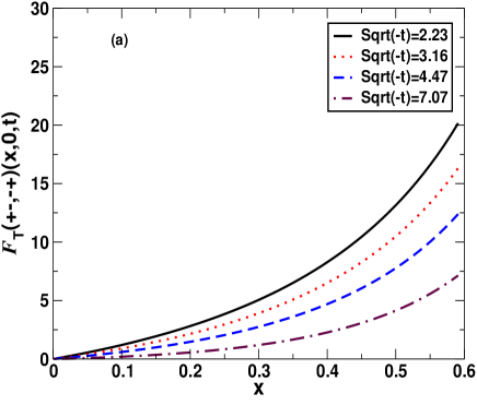
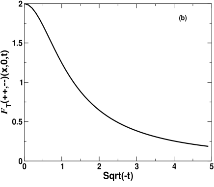
Figure 1: Plots of (a) $F_{T}(+-,-+)(x,0,t)=\left[H_{T}(x,0,t)+\frac{\sum_{i}\Delta_{i}^{2}}{4m^{2}}\tilde{H}_{T}(x,0,t)\right]$ as a function of $x$ for fixed values of $\sqrt{-t}$ in MeV and (b) $F_{T}(++,--)(x,0,t)=\left[E_{T}(x,0,t)+2\tilde{H}_{T}(x,0,t)\right]$ as a function of $\sqrt{-t}$ in MeV.

In order to extract different combinations of the chiral-odd GPDs of phenomenological importance, we combine the above results to get,

$${\cal F}^{1}_{T}(+-,-+)(x,0,t) = \frac{F^{1}_{T}(\uparrow\downarrow)+F^{1}_{T}(\downarrow\uparrow)}{2}=\left[H_{T}(x,0,t)+\frac{\Delta_{2}^{2}}{2m^{2}}\tilde{H}_{T}(x,0,t)\right]$$ (35)

$$= \frac{e^{2}}{(2\pi)^{3}}\frac{x}{1-x}\left[I_{1}+I_{2}+CI_{3}\right]\,$$

$${\cal F}^{2}_{T}(+-,-+)(x,0,t) = \frac{F^{2}_{T}(\uparrow\downarrow)-F^{2}_{T}(\downarrow\uparrow)}{2}=\left[H_{T}(x,0,t)+\frac{\Delta_{1}^{2}}{2m^{2}}\tilde{H}_{T}(x,0,t)\right]$$ (36)

$$= \frac{e^{2}}{(2\pi)^{3}}\frac{x}{1-x}\left[I_{1}+I_{2}+CI_{3}\right]\,$$

$${\cal F}^{1}_{T}(++,--)(x,0,t) = \frac{F^{1}_{T}(\uparrow\uparrow)+F^{1}_{T}(\downarrow\downarrow)}{2}=\left[E_{T}(x,0,t)+2\tilde{H}_{T}(x,0,t)\right]{-i\Delta_{2}\over 2m}$$ (37)

$$= \frac{e^{2}}{(2\pi)^{3}}m(1-x)^{2}(-i)\Delta_{2}I_{3}\,.$$

$${\cal F}^{2}_{T}(++,--)(x,0,t) = \frac{F^{2}_{T}(\uparrow\uparrow)+F^{2}_{T}(\downarrow\downarrow)}{2}=\left[E_{T}(x,0,t)+2\tilde{H}_{T}(x,0,t)\right]{i\Delta_{1}\over 2m}$$ (38)

$$= \frac{e^{2}}{(2\pi)^{3}}m(1-x)^{2}(i\Delta_{1})I_{3}\,.$$

The above equations show that $\tilde{H}_{T}(x,0,t)=0$ in this model. Analytic expressions for $H_{T}(x,0,t),E_{T}(x,0,t)$ and $\tilde{H}_{T}(x,0,t)$ are given in the appendix of metz in a quark model in terms of $k_{T}$ integrals, where $k_{T}$ is the transverse momentum of the quark. Apart from the overall color factors, our results agree with them.

In fig. 1 (a), we have plotted $H_{T}(x,0,t)+\frac{\sum_{i}\Delta_{i}^{2}}{4m^{2}}\tilde{H}_{T}(x,0,t)$ for fixed values of $t=-\Delta_{\perp}^{2}$ and as a function of $x$. It increases with x at fixed $t$, the magnitude decreases with increasing $\Delta_{\perp}^{2}$. We have taken ${e^{2}\over(2\pi)^{3}}=1$ and $m=0.5$ MeV. The helicity flip contributions depend on the scale $\Lambda$ which we have taken as $100$  MeV. This is similar to the unpolarized distribution dip ; dip2 . Note that the linear combination of the light-front helicity states here gives the overlap matrix element for the transversely polarized state. It is to be noted that both Eqs. (35) and (36) reduce to the transversity distribution $h_{1}(x)$ in the forward limit calculated in tran . Fig. 1(b) shows the plot of $E_{T}(x,0,t)+2\tilde{H}_{T}(x,0,t)$ as a function of $\sqrt{-t}$ in MeV. Note that this quantity becomes $x$ independent because of the $(1-x)^{2}$ present in the denominator of $I_{3}$. This is a particular feature of the model considered.

III Impact space representation

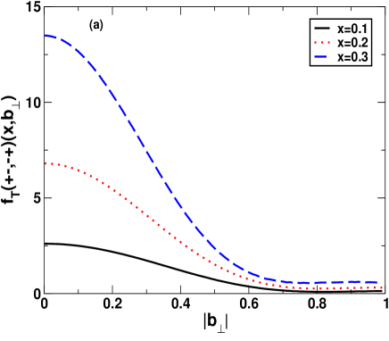
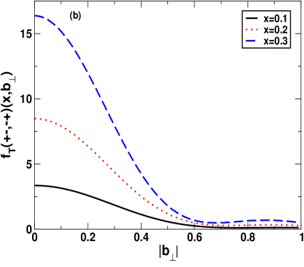
Figure 2: Impact parameter dependent pdfs $f_{T}(+-,-+)(x,b_{\perp})=\left[\mathcal{H}_{T}(x,b_{\perp})-\frac{\Delta_{b}}{4m^{2}}\tilde{\mathcal{H}}_{T}(x,b_{\perp})\right]$ as a function of $\mid b_{\perp}\mid$ for fixed values of $x$ at (a) $m=0.5$ MeV and (b) $m=0.8$ MeV. $\mid b_{\perp}\mid$ is in $\mathrm{MeV}^{-1}$.

The impact parameter dependent parton distributions are defined from the GPDs by taking a Fourier Transform (FT) in $\Delta_{\perp}$ as follows :

$$\mathcal{H}_{T}(x,b_{\perp}) = {1\over(2\pi)^{2}}\int d^{2}\Delta_{\perp}e^{-ib_{\perp}\cdot\Delta_{\perp}}H_{T}(x,0,-\Delta_{\perp}^{2})\,,$$

$$\mathcal{E}_{T}(x,b_{\perp}) = {1\over(2\pi)^{2}}\int d^{2}\Delta_{\perp}e^{-ib_{\perp}\cdot\Delta_{\perp}}E_{T}(x,0,-\Delta_{\perp}^{2})\,,$$

$$\tilde{\mathcal{H}}_{T}(x,b_{\perp}) = {1\over(2\pi)^{2}}\int d^{2}\Delta_{\perp}e^{-ib_{\perp}\cdot\Delta_{\perp}}\tilde{H}_{T}(x,0,-\Delta_{\perp}^{2})\,,$$

where $b_{\perp}$ is the impact parameter conjugate to $\Delta_{\perp}$.

We can write,

$$f_{T}(+-,-+)(x,b_{\perp}) = \int{d^{2}\Delta_{\perp}\over(2\pi)^{2}}e^{-ib_{\perp}.\Delta_{\perp}}\left[H_{T}(x,0,-\Delta_{\perp}^{2})+\frac{\Delta^{2}_{i}}{4m^{2}}\tilde{H}_{T}(x,0,-\Delta_{\perp}^{2})\right]$$ (42)

$$= \left[\mathcal{H}_{T}(x,b_{\perp})-\frac{\Delta_{b}}{4m^{2}}\tilde{\mathcal{H}}_{T}(x,b_{\perp})\right]$$

$$= \frac{e^{2}}{2(2\pi)^{3}}\frac{x}{1-x}\int_{0}^{\infty}\Delta d\Delta\left[log{\Lambda^{2}\over m^{2}(1-x)^{2}}\right.$$

$$\left.+log{\Lambda^{2}\over(m^{2}+\Delta^{2}_{\perp})(1-x)^{2}}+C\int_{0}^{1}{d\alpha\over D}\right]J_{0}(b\Delta)\,.$$

where

$$\Delta_{b}f={\partial\over\partial b_{i}}{\partial\over\partial b_{i}}f\,.$$ (43)

$J_{0}(b\Delta)$ is the Bessel function. In fig. 2 we have plotted $f_{T}(+-,-+)(x,b_{\perp})$ as a function of $b_{\perp}$ for fixed $x$ for two different values of the mass parameter $m$. It is peaked at $b_{\perp}=0$ and falls away further from it. The peak increases as $x$ increases. This quantity describes the correlation between the transverse quark spin and the target spin in a transversely polarized nucleon in impact parameter space. For an elementary Dirac particle, this would be a delta function at $b_{\perp}=0$. The smearing in transverse position space occurs due to the two-particle LFWF.

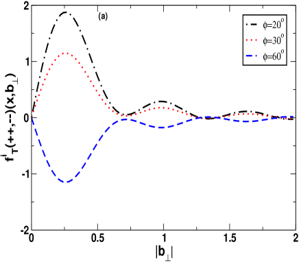
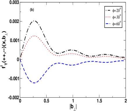
Figure 3: Impact parameter dependent pdfs $f^{i}_{T}(++,--)(x,b_{\perp})=-\epsilon^{ij}b_{j}{\partial\over\partial B}\left[\mathcal{E}_{T}(x,b_{\perp})+2\tilde{\mathcal{H}}_{T}(x,b_{\perp})\right]$ as a function of $\mid b_{\perp}\mid$ for different values of $\phi$ and (a) $m=0.5$ MeV and (b) $m=0.01$ MeV . $\mid b_{\perp}\mid$ is in $\mathrm{MeV}^{-1}$.

The transversity density of quarks is defined as

$$\delta^{i}q(x,b_{\perp})=-{\epsilon^{ij}\over m}b_{j}{\partial\over\partial b^{2}}(2\tilde{\mathcal{H}}_{T}+\mathcal{E}_{T})$$ (44)

Even for an unpolarized target, it can be non-zero (as shown in burchi using in a simple model). This is due to spin-orbit correlations in the quark wave function. If the quarks have orbital angular momentum then their distribution is shifted to one side. In an unpolarized nucleon, all orientations are equally probable and therefore, the unpolarized distribution is axially symmetric. However, if there is a spin-orbit correlation, then quarks with a certain spin orientation will shift to one side and those with a different orientation will shift to another side.

This can be constructed from,

$$f^{i}_{T}(++,--)(x,b_{\perp}) = -\epsilon^{ij}b_{j}{\partial\over\partial B}\left[\mathcal{E}_{T}(x,b_{\perp})+2\tilde{\mathcal{H}}_{T}(x,b_{\perp})\right]$$ (45)

$$= i\epsilon^{ij}\int{d^{2}\Delta_{\perp}\over(2\pi)^{2}}\Delta_{j}e^{-ib_{\perp}.\Delta_{\perp}}\left[E_{T}(x,0,-\Delta_{\perp}^{2})+2\tilde{H}_{T}(x,0,-\Delta_{\perp}^{2})\right],$$

$$= -i{\epsilon^{ij}b_{j}\over b}\int{(\Delta)^{2}\,d\Delta\over(2\pi)}\left[E_{T}(x,0,-\Delta_{\perp}^{2})+2\tilde{H}_{T}(x,0,-\Delta_{\perp}^{2})\right]J_{1}(b\Delta)\,,$$

where ${\partial\over\partial B}=2{\partial\over\partial b^{2}}$ and

$$b_{1}=b\cos\phi\,,~{}~{}~{}~{}~{}~{}b_{2}=b\sin\phi\,.$$ (46)

For computational purpose, we have used

$$J_{n}(b\Delta)={1\over\pi}\int_{0}^{\pi}d\theta\cos(n\theta-b\Delta\sin\theta).$$ (47)

In Fig. 3, we have plotted $f^{i}_{T}(++,--)(x,b_{\perp})$ as a function of $b_{\perp}$ for different values of $\phi$. As stated before, in the simple model we consider, this quantity is independent of $x$. We took the constant phase factor $(-i)$ out. The effect of this term is to shift the peak of the impact parameter space density (see eq. (8) of chiral ) away from $b_{\perp}=0$. This shift clearly shows the interplay between the spin and the orbital angular momentum of the constituents of the two-particle LFWF. In order to understand the plots, consider a two-dimensional plane with $b_{1}$ and $b_{2}$ plotted along the two axes. Fixed $\mid b_{\perp}\mid$ denote concentric circles in this plane. From our plots, we see that the position of the peak of $f_{T}^{i}$ is indepenent of $\phi$ and $m$. The magnitude of the peak increases as $m$ increases. The magnitude and sign changes as $\phi$ changes. $f_{T}^{i}$ would vanish at $\phi={\pi\over 4}$ and ${5\pi\over 4}$. In 2-D $b_{1}-b_{2}$ plane, the primary peak will lie on a circle and the secondary peak will lie on a concentric circle with larger radius.

IV conclusion

In this work, we have studied the chiral-odd GPDs in impact parameter space in a self consistent relativistic two-body model, namely for the quantum fluctuation of an electron at one loop in QED. In its most general form drell , this model can act as a template for the quark-spin one diquark light front wave function for the proton, although not numerically. Working in light-front gauge, we expressed the GPDs as overlaps of the light-front wave functions. We took the skewness to be zero. Only the diagonal $2\to 2$ overlap contributes in this case. The impact space representations are obtained by taking Fourier transform of the GPDs with respect to the transverse momentum transfer. It is known chiral ; burchi that certain combinations of the chiral-odd GPDs in impact parameter space affect the quark and nucleon spin correlations in different ways. For example, the combination $\mathcal{H}_{T}-{\Delta_{b}\over 4m^{2}}\tilde{\mathcal{H}}_{T}$ gives the correlation between the transverse quark spin and the target spin in a transversely polarized nucleon. On the other hand, the quantity $\epsilon_{ij}b_{j}{\partial\over\partial B}(\mathcal{E}_{T}+2\tilde{\mathcal{H}}_{T})$ gives the spin-orbit correlation of the quarks in the nucleon. We have investigated both and have shown that due to the interplay between the spin and orbital angular momentum of the 2-particle LFWF, the distribution in the impact parameter space is shifted sideways. In a future work, we plan to investigate the various positivity constraints for the chiral-odd GPDs as well as the effect of non-zero skewness $\xi$, when there is a finite momentum transfer in the longitudinal direction as well.

V acknowledgment

AM thanks DST Fasttrack scheme, Govt. of India for financial support for completing this work.

References

(1) For reviews on generalized parton distributions,
and DVCS, see M. Diehl,
Phys. Rept, 388, 41 (2003); A. V. Belitsky and A. V. Radyushkin, Phys.
Rept. 418 1, (2005); K. Goeke, M.
V. Polyakov, M. Vanderhaeghen, Prog. Part. Nucl. Phys. 47, 401 (2001).
(2) M. Burkardt, Int. Jour. Mod. Phys. A 18, 173 (2003);
M. Burkardt, Phys. Rev. D 62, 071503 (2000), Erratum-
ibid, D 66, 119903 (2002); J. P. Ralston and B. Pire, Phys. Rev. D 66, 111501 (2002).
(3) D. E. Soper, Phys. Rev. D 15, 1141 (1977).
(4) M. Burkardt, Phys. Rev D 72, 094021 (2005).
(5) X. Ji. Phys. Rev. Lett. 78, 610 (1997).
(6) M. Diehl, Eur. Phys. J. C 19, 485 (2001).
(7) M. Diehl and P. Hagler, Eur.Phys.J.C 44, 87
(2005).
(8) D. Yu Ivanov, B. Pire, L. Szymanowski, O. V. Teryaev, Phys.
Lett. B 550, 65 (2002); Phys. Part. Nucl. 35, 67
(2004).
(9) B. Pasquini, M. Pincetti, S. Boffi, Phys. Rev. D 72,
094029 (2005).
(10) S. J. Brodsky and S. D. Drell, Phys. Rev. D 22, 2236
(1980).
(11) A. Harindranath, R. Kundu, W. M. Zhang, Phys.
Rev. D 59, 094013 (1999); A. Harindranath, A. Mukherjee,
R. Ratabole, Phys. Lett. B 476, 471 (2000); Phys. Rev.
D 63, 045006 (2001).
(12) D. Chakrabarti and A. Mukherjee, Phys. Rev. D 71, 014038
(2005).
(13) D. Chakrabarti, A. Mukherjee, Phys. Rev. D 72,
034013 (2005).
(14) A. Mukherjee and M. Vanderhaeghen, Phys. Lett. B 542, 245 (2002);
Phys. Rev. D 67, 085020 (2003).
(15) S. J. Brodsky, D. Chakrabarti, A. Harindranath, A.
Mukherjee, J. P. Vary, Phys. Lett. B, 641, 440 (2006), Phys. Rev. D 75, 0143003 (2007).
(16) S. J. Brodsky, D. S. Hwang, B-Q. Ma, I. Schmidt, Nucl. Phys.
B 593, 311 (2001).
(17) S. J. Brodsky, M. Diehl, D. S. Hwang, Nucl. Phys. B
596, 99 (2001); M. Diehl, T. Feldmann, R. Jacob, P. Kroll, Nucl. Phys.
B 596, 33 (2001), Erratum-ibid 605, 647 (2001).
(18) W. M. Zhang, A. Harindranath, Phys. Rev. D 48, 4881
(1993).
(19) A. Mukherjee and D. Chakrabarti,
Phys. Lett. B 506, 283 (2001).
(20) H. Dahiya, A. Mukherjee, S. Ray, Phys. Rev. D 76, 034010
(2007).
(21) D. W. Sivers, Phys. Rev. D 43, 261 (1991).
(22) M. Burkardt, Phys. Rev. D 66, 114005 (2002).
(23) D. Boer and P. J. Mulders, Phys. Rev. D 57, 5780
(1998).
(24) S. Meissner, A. Metz and K. Goeke, hep-ph/0703176.