Improving the Calibration of Type Ia Supernovae
Using Late-time Lightcurves

Abstract

The use of Type Ia supernovae (SNe Ia) as cosmological standard candles is a key to solving the mystery of dark energy. Improving the calibration of SNe Ia increases their power as cosmological standard candles. We find tentative evidence for a correlation between the late-time lightcurve slope and the peak luminosity of SNe Ia in the $B$ band; brighter SNe Ia seem to have shallower lightcurve slopes between 100 and 150 days from maximum light. Using a Markov Chain Monte Carlo (MCMC) analysis in calibrating SNe Ia, we are able to simultaneously take into consideration the effect of dust extinction, the luminosity and lightcurve width correlation (parametrized by $\Delta m_{15}$), and the luminosity and late-time lightcurve slope correlation. For the available sample of 11 SNe Ia with well-measured late-time lightcurves, we find that correcting for the correlation between luminosity and late-time lightcurve slope of the SNe Ia leads to an intrinsic dispersion of 0.12 mag in the Hubble diagram. Our results have significant implications for future supernova surveys aimed to illuminate the nature of dark energy.

1 Introduction

One of the most important problems in cosmology today is to solve the mystery of dark energy, the unknown reason for the observed cosmic acceleration (Riess et al., 1998; Perlmutter et al., 1999). The discovery of cosmic acceleration was made using Type Ia Supernovae (SNe Ia), as SNe Ia can be calibrated to be good cosmological standard candles (Phillips, 1993; Riess, Press, & Kirshner, 1995). Improving the calibration of SNe Ia increases their power as cosmological standard candles.

A SN Ia is a thermonuclear explosion that completely destroys a carbon/oxygen white dwarf as it approaches the Chandrasekher limit of 1.4 $M_{\odot}$. This is the reason SNe Ia can be calibrated to be good standard candles. The first challenge to overcome when using SNe Ia as cosmological standard candles is properly incorporating the intrinsic scatter in SN Ia peak luminosity. The usual calibration of SNe Ia reduces the intrinsic scatter in SN Ia peak luminosity to about 0.17 mag (Phillips, 1993; Riess, Press, & Kirshner, 1995). The calibration techniques used so far are based on one observable parameter, the lightcurve width, which can be parametrized either as $\Delta m_{15}$ (decline in magnitudes in the $B$-band for a SN Ia in the first 15 SN Ia restframe days after $B$-band maximum, see Phillips (1993)), or a stretch factor (which linearly scales the time axis, see Goldhaber et al. (2001)). The lightcurve width is associated with the amount of ⁵⁶Ni produced in the SN Ia explosion, which in turn depends on when the carbon burning makes the transition from turbulent deflagration to a supersonic detonation (Wheeler, 2003).

There are theoretical reasons to expect the existence of additional physical parameters that characterize the lightcurve of a SN Ia. For example, Milne, The, & Leising (2001) modeled the late light curves of SNe Ia, and found that the nonlocal and time-dependent energy deposition due to the transport of Comptonized electrons can produce a 0.10 to 0.18 mag correction to the late-time brightness of SNe Ia, depending on their position in the $\Delta m_{15}$ sequence.

In this paper we show that late-time lightcurves of SNe Ia can be used to tighten the calibration of SNe Ia, and reduce their effective (post-calibration) intrinsic scatter in the Hubble diagram. We describe our method in Section 2, and present our results in Section 3. We summarize and conclude in Section 4.

2 Method

2.1 Defining the sample

We use the lightcurve fits obtained using the Joint SuperStretch code for SN Ia lightcurves (Wang et al., 2006) to derive the lightcurve parameters (epoch and apparent magnitudes at maximum light and $\Delta m_{15}$). This is necessary for consistency in making color and $\Delta m_{15}$ corrections.

We select a sample of “normal” SNe Ia (from a total of 135 available) that satisfy the following requirements:

(1) $B_{max}-V_{max}\leq 0.5$;
(2) $0.015<z<.1$;
(3) B lightcurve data extending beyond 100 days from maximum light.

The requirement of $B_{max}-V_{max}\leq 0.5$ selects the “Branch normal” SNe Ia (Vaughan et al., 1995; Branch, 1998), which is standard in studying SNe Ia as cosmological standard candles. The requirement of $0.015<z<.1$ selects SNe Ia which are nearby yet distant enough so that they are not affected by peculiar velocities due to cosmic large scale structure that modifies the Hubble diagram of nearby standard candles (Wang, Spergel, & Turner, 1998), which has the largest impact on the nearest SNe Ia (see, e.g., Zehavi et al. (1998); Cooray & Caldwell (2006); Hui & Greene (2006); Conley et al. (2007)).

This yields a sample of 13 SNe Ia. Of these, we exclude two more SNe: SN1999cc and SN1993h. SN1999cc has only one data point in the B lightcurve between 40 and 100 days from maximum light, insufficient to determine a slope independent of the lightcurve model. For SN1993h, the late-time lightcurve slope appears to depend on the lightcurve model, due to the appearance of a small secondary peak in the lightcurve data at $\sim$ 80 days from maximum light. For the final set of 11 SNe Ia, the B lightcurves are very close to a straight line at $\gtrsim$ 60 days from maximum light in the SN Ia restframe, and there are a minimum of two data points at $t\gtrsim 60$ days from maximum light.

Our final sample consists of 11 SNe Ia that have lightcurve data at $\gtrsim$ 100 days from maximum light in the SN Ia restframe, and late-time lightcurve slopes insensitive to the lightcurve model. Table 1 lists the SNe Ia in our sample. We include all the data that are required to allow others to reproduce our results. Note that $\Delta b_{lt}$ and $N_{lt}$ are not required to reproduce our results [see Eqs.(4)-(5)], but are given for reference.

Table 1: Nearby SNe Ia with well defined late-time lightcurves.

SN name	$z$	$B_{max}$	$\Delta B_{max}$	$V_{max}$	$\Delta m_{15}$	$b_{lt}$	$\Delta b_{lt}$	$N_{lt}$	reference
SN1990O	0.031	16.607	0.035	16.533	0.961	0.0160	0.0008	4	H96b
SN1990T	0.040	17.454	0.086	17.537	1.298	0.0152	0.0028	6	H96b
SN1990Y	0.039	17.674	0.306	17.494	1.217	0.0153	0.0025	7	H96b
SN1992bc	0.020	15.207	0.009	15.207	0.960	0.0147	0.0002	10	H96b
SN1993ag	0.050	18.298	0.026	18.081	1.382	0.0142	0.0030	3	H96b
SN1997dg	0.033	17.143	0.033	17.117	1.281	0.0177	–	2	J06
SN1998ec	0.020	16.670	0.053	16.406	1.074	0.0164	0.0033	4	J06
SN1998V	0.017	15.912	0.029	15.738	1.150	0.0163	0.0012	5	J06
SN1999ef	0.038	17.524	0.117	17.418	1.055	0.0160	0.0049	3	J06
SN2000dk	0.016	15.637	0.021	15.543	1.457	0.0136	0.0029	4	J06
SN2000fa	0.022	16.026	0.051	16.055	1.140	0.0164	0.0028	4	J06

2.2 Fitting the Absolute Magnitudes

To convert observed apparent magnitudes to absolute magnitudes we assume a flat universe, with $\Omega_{m}=0.3$, $\Omega_{\Lambda}=0.7$, and $H_{0}=70\,$km s${}^{-1}\,$Mpc^-1. The B absolute magnitudes are

$$M_{B}^{obs}\equiv B_{max}-\mu,$$ (1)

where $B_{max}$ denotes the apparent magnitude at peak brightness in the B band, and the distance modulus $\mu$ is

$$\mu(z)=m-M=5\log\left[d_{L}(z)/10{\,{\mbox{pc}}}\right].$$ (2)

For $z<0.1$, the luminosity distance $d_{L}(z)$ is well approximated by

$$d_{L}(z)=\frac{cz}{H_{0}}\,\left[1+\frac{1}{2}(1-q_{0})\,z\right],$$ (3)

with $q_{0}=\Omega_{m}/2-\Omega_{\Lambda}$. Since we are only considering very low redshift SNe Ia, our results are insensitive to the assumed cosmological model.

Without any corrections, the dispersion of the SNe Ia in our sample in the Hubble diagram is 0.35 mag (see Fig.5(a)). This is due to extinction by dust, as well as the intrinsic dispersion in the luminosities of SNe Ia due to the physical diversity of these objects (Woosley et al., 2007). Our goal is to model these effects phenomenologically using observational data, in order to calibrate SNe Ia into good standard candles.

According to Cardelli, Clayton, & Mathis (1989), due to dust extinction, all true B magnitudes differ from the observed B magnitudes by $\delta B\equiv B-B^{obs}=R_{B}\,\delta(B-V)$, where $\delta(B-V)\equiv(B-V)-(B-V)^{obs}$, and $R_{B}$ is approximately constant. Following van den Bergh (1995), we use ${\cal R}$ to denote the color correction coefficient parametrizing the combined effects of dust extinction and intrinsic SN color variation. Assuming that $B_{max}-V_{max}=0$ for unreddened SNe Ia (Phillips et al., 1999), the dust correction to $M_{B}^{obs}$ is ${\cal R}E$, with $E=B_{max}-V_{max}$.

There is a well known correlation between SN Ia peak luminosity and $\Delta m_{15}$, the decline in brightness (in units of mag) 15 days (in the SN restframe) after peak brightness (Phillips, 1993). Following Wang et al. (2006), we parametrize the $\Delta m_{15}$ dependence of $M_{B}^{obs}$ with a piecewise linear function, ${\cal D}(\Delta m_{15})=\alpha\,\left(\Delta m_{15}-1.1\right)+\alpha\prime\,\left|\Delta m_{15}-1.1\right|$.

We use the Markov Chain Monte Carlo (MCMC) technique (see Neil (1993) for a review), illustrated for example in Lewis & Bridle (2002), in the likelihood analysis. The MCMC method scales approximately linearly in computation time with the number of parameters. The method samples from the full posterior distribution of the parameters, and from these samples the marginalized posterior distributions of the parameters can be estimated. In the MCMC analysis, we fit $M_{B}^{obs}$ to

$$M_{B}^{fit}=M+\Delta M^{cor}=M+{\cal R}E+\alpha\,\left(\Delta m_{15}-1.1\right)+\alpha\prime\,\left|\Delta m_{15}-1.1\right|+\beta b_{lt},$$ (4)

where $b_{lt}$ (in units of mag/day) is the late-time lightcurve slope (in the SN restframe). In our MCMC code, we use

$$\chi^{2}=\sum_{i=1}^{N}\left(\frac{M_{B}^{obs}(z_{i})-M_{B}^{fit}(z_{i})}{\Delta B_{max}(z_{i})}\right)^{2}.$$ (5)

The MCMC algorithm allows us to explore the dependence of $M_{B}^{obs}$ on all the parameters simultaneously.

The Hubble diagram dispersion is a conventional measure of the intrinsic scatter of SNe Ia. It is given by the standard deviation of the apparent magnitudes at maximum light of the SNe Ia, $B_{max}$, from the theoretical predictions given by

$$m_{0}(z)\equiv\mu(z)+M,$$ (6)

where $M$ is a constant that denotes the absolute magnitude of SNe Ia. It can only be determined through direct measurements of the distances to the SNe Ia using Cepheid variable stars. Since $M$ has no impact on the relative calibration of SNe Ia that we study in this paper, we allow $M$ to vary in order to obtain the smallest scatter in the Hubble diagram, independent of the $M$ values obtained in the MCMC likelihood analysis. This is the same approach adopted by Wang et al. (2006) using a different likelihood analysis technique.

3 Results

We have used the restframe fitted lightcurves to obtain slopes of the lightcurves at late-time, chosen to be between 100 and 150 days from maximum light. Since the lightcurves are very close to straight lines at $\gtrsim 60\,$days from maximum light, the measured slopes are robust and not sensitive to the lightcurve model. Table 1 lists the late-time lightcurve slopes $b_{lt}$ for the SNe Ia in our sample.

Our data consist of ($B_{max}$, $\Delta B_{max}$, $E$, $\Delta m_{15}$, $b_{lt}$) for each of the SNe Ia in our sample. The parameters that we vary in our MCMC likelyhood analysis are ($M$, ${\cal R}$, $\alpha$, $\alpha\prime$, $\beta$). Wang et al. (2006) found that ${\cal R}=2.59\pm 0.24$, $\alpha=0.78\pm 0.09$, and $\alpha\prime=-0.54\pm 0.19$. To avoid obtaining unphysical values of $\alpha$ and $\alpha\prime$ due to the small size of our sample, we impose a prior of $\alpha\prime\geq-2$ in our analysis.

We obtain millions of MCMC samples, which are then appropriately thinned for statistical independence. We do not present results on the “nuisance” parameter $M$; it is marginalized over in obtaining the probability distributions that we present. Fig.1 shows the marginalized probability density functions (pdf) of ${\cal R}$, $\alpha$, $\alpha\prime$, and $\beta$. Fig.2 shows the corresponding 2-D joint confidence contours (68% and 95%) for these parameters. For comparison, Fig.3 and Fig.4 show the pdf and joint confidence contours for ${\cal R}$, $\alpha$, and $\alpha\prime$, with $\beta=0$. Fig.5 and Fig.6 show the pdf and joint confidence contours for $\alpha$, $\alpha\prime$, and $\beta$, for fixing ${\cal R}=4.1$ (standard Milky-Way dust). In Fig.1, Fig.3, and Fig.5, the dotted lines are the likelihood functions. Agreement between the pdf and the likelihood function indicates that the MCMC chains have converged and hence provide reliable pdf’s. Table 2 lists the best fit, mean, and standard deviations for ${\cal R}$, $\alpha$, $\alpha\prime$, $\beta$.

Figure 1: Marginalized probability density functions (pdf) of ${\cal R}$, $\alpha$, $\alpha\prime$, and $\beta$.

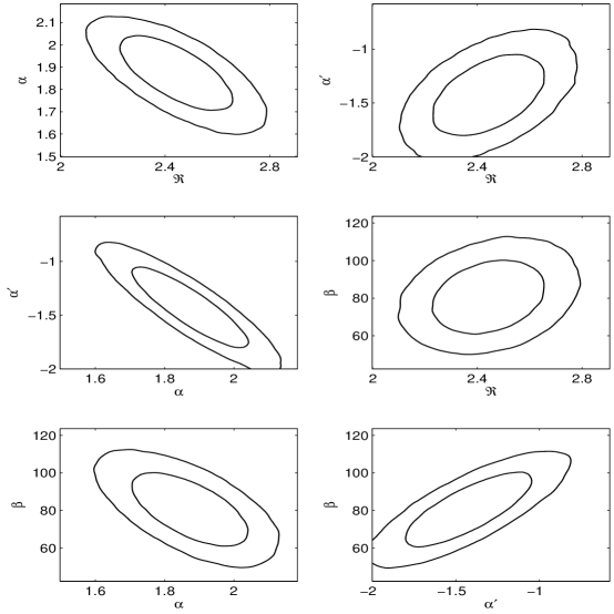
Figure 2: 2-D joint confidence level contours (68% and 95%) corresponding to Fig.1.

Figure 3: Marginalized probability density functions (pdf) of ${\cal R}$, $\alpha$, and $\alpha\prime$, for $\beta=0$.

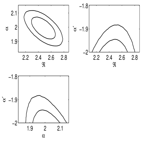
Figure 4: 2-D joint confidence level contours (68% and 95%) corresponding to Fig.3.

Figure 5: Marginalized probability density functions (pdf) of $\alpha$, and $\alpha\prime$, and $\beta$, for fixing ${\cal R}=4.1$ (standard Milky-Way dust).

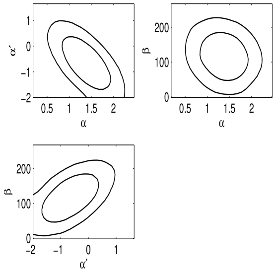
Figure 6: 2-D joint confidence level contours (68% and 95%) corresponding to Fig.5.

Table 2: Best fit, mean, and standard deviations for ${\cal R}$, $\alpha$, $\alpha\prime$, $\beta$.

parameter	best fit	mean	rms dev
	including $b_{lt}$:
${\cal R}$	2.407	2.445	0.141
$\alpha$	1.890	1.870	0.109
$\alpha\prime$	$-$1.453	$-$1.418	0.244
$\beta$	77.490	80.925	12.779
	not including $b_{lt}$	($\beta=0$):
${\cal R}$	2.454	2.480	0.123
$\alpha$	2.007	1.994	0.051
$\alpha\prime$	$-$2.000	$-$1.969	0.030
	forcing ${\cal R}=4.1$:
$\alpha$	1.372	1.371	0.345
$\alpha\prime$	$-$0.583	$-$0.621	0.633
$\beta$	112.364	117.889	43.939

It is reassuring that we obtain the same value of ${\cal R}$ whether or not we include late-time lightcurve slope $b_{lt}$ in our analysis. Note that the prior of $\alpha\prime\geq-2$ has little impact if we include $b_{lt}$ in our analysis (see Figs.1-2), but it has a very large impact if we only fit for ($M$, ${\cal R}$, $\alpha$, $\alpha\prime$). This indicates that the set of parameters ($M$, ${\cal R}$, $\alpha$, $\alpha\prime$) does not properly describe the data, given reasonable physical priors on $\alpha\prime$.

Fig.7 shows the Hubble diagrams for three cases, with the solid line indicating $m_{0}(z)=\mu(z)+M$ in each case, where $M$ is obtained by minimizing the rms of $|B_{max}(z)-m_{0}(z)|$ (the Hubble diagram dispersion). The three cases are: (a) No corrections. (b) $B_{max}$ corrected by subtracting $\Delta M^{cor}={\cal R}E+\alpha\,\left(\Delta m_{15}-1.1\right)+\alpha\prime\,\left|\Delta m_{15}-1.1\right|$, with ${\cal R}=2.45$, $\alpha=2.01$, and $\alpha\prime=-2.00$. (c) $B_{max}$ corrected by subtracting $\Delta M^{cor}={\cal R}E+\alpha\,\left(\Delta m_{15}-1.1\right)+\alpha\prime\,\left|\Delta m_{15}-1.1\right|+\beta b_{lt}$, with ${\cal R}=2.41$, $\alpha=1.89$, $\alpha\prime=-1.45$, and $\beta=77.49$ (mag/day)^-1. The parameter values in (b) and (c) correspond to the best fit values from the MCMC analysis (listed in Table 2). We find that including the correlation between luminosity and late-time lightcurve slope in correcting $M_{B}^{obs}$ reduces the Hubble diagram dispersion from 0.14 mag to 0.12 mag. For comparison, fixing ${\cal R}=4.1$ (standard Milky-Way dust) gives a Hubble diagram dispersion of 0.22 mag. This indicates that the assumption of standard Milky-Way dust is not supported by the data.

Figure 7: Hubble diagrams for three cases, with the solid line indicating $m_{0}(z)=\mu(z)+M$ in each case, where $M$ is obtained by minimizing the rms of $|B_{max}(z)-m_{0}(z)|$ (the Hubble diagram dispersion). (a) No corrections. (b) $B_{max}$ corrected by subtracting $\Delta M^{cor}={\cal R}E+\alpha\,\left(\Delta m_{15}-1.1\right)+\alpha\prime\,\left|\Delta m_{15}-1.1\right|$, with ${\cal R}=2.45$, $\alpha=2.01$, and $\alpha\prime=-2.00$. (c) $B_{max}$ corrected by subtracting $\Delta M^{cor}={\cal R}E+\alpha\,\left(\Delta m_{15}-1.1\right)+\alpha\prime\,\left|\Delta m_{15}-1.1\right|+\beta b_{lt}$, with ${\cal R}=2.41$, $\alpha=1.89$, $\alpha\prime=-1.45$, and $\beta=77.49$ (mag/day)^-1. For comparison, fixing ${\cal R}=4.1$ (standard Milky-Way dust) gives a Hubble diagram dispersion of $\sigma=0.22$ mag, much larger than the Hubble diagram dispersions in panels (b) and (c).

To study the effect of the measurement uncertainty in $B_{max}$ for our sample, we have repeated our MCMC analysis setting $\Delta B_{max}$ to a constant. This gives similar results as above. We find that including the correlation between luminosity and late-time lightcurve slope in correcting $M_{B}^{obs}$ reduces the Hubble diagram dispersion from 0.13 mag to 0.11 mag. This is similar to what we find when using the actual $\Delta B_{max}$ from Table 1.

Fig.8 shows the absolute magnitude corrected for color and $\Delta m_{15}$ only [case (b) of Fig.7], versus $b_{lt}$, with its coefficient $\beta$ given by case (c) of Fig.7. This shows that the evidence for the correlation between luminosity and late-time lightcurve slope is tentative due to the small size of the sample. A much larger sample of SNe Ia with well measured late-time lightcurves is needed to firmly establish this correlation.

Figure 8: The absolute magnitude corrected for color and $\Delta m_{15}$ only [case (b) of Fig.7], versus the late-time lightcurve slope $b_{lt}$, with its coefficient $\beta$ given by case (c) of Fig.7.

4 Discussion and Summary

Improving the calibration of SNe Ia increases the power of SNe Ia as cosmological standard candles. We have shown the tentative evidence for a correlation between SN Ia peak luminosity and late-time lightcurve slope in the $B$ band; brighter SNe Ia have shallower lightcurve slopes between 100 and 150 days from maximum light (see Fig.8). Using this correlation, we are able to reduce the intrinsic scatter of SNe Ia (measured by the Hubble diagram residue) to 0.12 mag (see Fig.7).

We use the MCMC algorithm in our likelihood analysis; this allows us to explore all the parameters simultaneously and efficiently in calibrating the SN Ia peak luminosity for our sample of SNe Ia. We only used $\Delta B_{max}$ in calculating $\chi^{2}$, since including the errors in color, $\Delta m_{15}$, and late-time lightcurve slope introduces spurious pdfs in the MCMC analysis. Our results are not sensitive to the uncertainty in $B_{max}$ (setting $\Delta B_{max}$ to a constant gives similar results to using the $\Delta B_{max}$ from Table 1). The parameter set is ($M$, ${\cal R}$, $\alpha$, $\alpha\prime$, $\beta$), which contains the nuisance parameter and correction coefficients for color, $\Delta m_{15}$, and late-time lightcurve slope respectively. The pdf’s we have found for (${\cal R}$, $\alpha$, $\alpha\prime$, $\beta$) are very close to being Gaussian (see Fig.1 and Fig.3), except for the pdf’s for $\alpha\prime$ (which are cutoff by the prior of $\alpha\prime\geq-2$). Late-time lightcurve slope $b_{lt}$ appears uncorrelated with color (see Fig.2), which supports $b_{lt}$ being an intrinsic observable that correlates with the peak luminosity of SNe Ia.

The apparent correlation between peak luminosity and late-time lightcurve slope in the $B$ band that we have found is consistent with the results by Cappellaro et al. (1997). They studied the late-time lightcurves of five SNe Ia in the $V$ band with the focus of modeling lightcurves at very late times (later than 150-200 days from maximum light), and found a similar trend in the peak luminosity and late-time lightcurve slope (which they parametrized with the difference in $V$ magnitude from maximum to 300 days, see Table 1 of Cappellaro et al. (1997)).

The coefficients for correcting for the correlation between decline-rate and peak luminosity that we have found are very different from previous work (see Table 2 and Phillips (1993); Hamuy et al. (1996a); Phillips et al. (1999); Wang et al. (2006)). This is likely partly a consequence of the particular sample of 11 SNe Ia we have used for our analysis. This is not surprising, since previous work by various groups also found very different $\Delta m_{15}$ corrections (Phillips et al., 1999; Wang et al., 2006), indicating that this correction is highly sensitive to sample selection.

Note that the color correction coefficient we found was not sensitive to whether we correct for late-time lightcurve slope, and is consistent with the color correction coefficient of ${\cal R}=2.59\pm 0.24$ found by Wang et al. (2006). This is very different from a coefficient of ${\cal R}=4.1$ that is typical of Milky Way dust. We found that fixing ${\cal R}=4.1$ gives a Hubble diagram residue almost twice as large as the Hubble diagram residue found when allowing ${\cal R}$ to vary (see Fig.7 and its caption). This strengthens the evidence that the color correction coefficient ${\cal R}$ of SN data cannot be explained by extinction by typical Milky-Way dust. The deviation of ${\cal R}$ from ${\cal R}=4.1$ could be due to the mixing of intrinsic SN Ia color variation with dust extinction (Conley et al., 2007), or variations in the properties of dust. The definitive resolution of this issue will likely require NIR observations of a large number of SNe Ia (Krisciunas, Phillips, & Suntzeff, 2004; Phillips et al., 2006).

Our results show the benefit of extending the observations of SN Ia lightcurves beyond 100 days in the SN Ia restframe, with several data points between 50 to 150 days to enable a robust measurement of the late-time lightcurve slope. Our sample only contains 11 SNe Ia, limited by currently available data. The expansion in the scope of SN observations to obtain late-time lightcurves is straightforward for surveys which cover the same areas in the sky in regular intervals (Wang, 2000; Phillips et al., 2006).

Our results have significant implications for the survey strategy of future SN surveys, such as those planned for the Advanced Liquid-mirror Probe for Astrophysics, Cosmology and Asteroids (ALPACA); Pan-STARRS; the Dark Energy Survey (DES); the Large Synoptic Survey Telescope (LSST), and the Joint Dark Energy Mission (JDEM).

Acknowledgments We are grateful to Lifan Wang for providing the lightcurve fits to the SN data we used, Alex Conley for sending us his compilation of nearby SN data, and David Branch for helpful discussions and comments on drafts of the manuscript. This work was supported in part by the NSF CAREER grant AST-0094335 and AST 05-06028.

References

- Branch (1998) Branch, D. 1998, ARA & A, 36, 17
- Cappellaro et al. (1997) Cappellaro, E., et al. 1997, A&A, 328, 203
- Cardelli, Clayton, & Mathis (1989) Cardelli, J.A.; Clayton, G.C.; & Mathis, J.S. 1989, ApJ, 345, 245
- Conley et al. (2007) Conley, A., et al. 2007, arXiv:0705.0367v2, ApJL, in press
- Cooray & Caldwell (2006) Cooray, A.; Caldwell, R.R. 2006, Phys.Rev.D73, 103002
- Goldhaber et al. (2001) Goldhaber, G., et al. 2001, ApJ, 558, 359
- Hamuy et al. (1996a) Hamuy, M., et al. 1996a, AJ, 112, 2391
- Hamuy et al. (1996b) Hamuy, M., et al. 1996b, AJ, 112, 2408
- Howell et al. (2006) Howell, D. A., et al. 2006, Nature 443, 308
- Hui & Greene (2006) Hui, L.; & Greene, P.B. 2006, Phys. Rev. D73, 123526
- Jha et al. (2006) Jha, S., et al. 2006, AJ, 131, 527
- Krisciunas, Phillips, & Suntzeff (2004) Krisciunas, K.; Phillips, M.M.; Suntzeff, N.B. 2004, ApJ, 602, L81
- Lewis & Bridle (2002) Lewis, A., & Bridle, S. 2002, PRD, 66, 103511
- Milne, The, & Leising (2001) Milne, P. A.; The, L.-S.; Leising, M. D. 2001, ApJ, 559, 1019
- Neil (1993) Neil, R.M. 1993, ftp://ftp.cs.utoronto.ca/pub/ radford/review.ps.gz
- Perlmutter et al. (1999) Perlmutter, S. et al., 1999, ApJ, 517, 565
- Phillips (1993) Phillips, M.M. 1993, ApJ, 413, L105
- Phillips et al. (1999) Phillips, M. M., et al. 1999, AJ, 118, 1766
- Phillips et al. (2006) Phillips, M. M.; Garnavich, P.; Wang, Y. et al. 2006, Proc. of SPIE, Volume 6265, 626529, arXiv:astro-ph/0606691v1
- Press et al. (1994) Press, W.H., Teukolsky, S.A., Vettering, W.T., & Flannery, B.P. 1994, Numerical Recipes, Cambridge University Press, Cambridge.
- Riess, Press, & Kirshner (1995) Riess, A.G., Press, W.H., and Kirshner, R.P. 1995, ApJ, 438, L17
- Riess et al. (1998) Riess, A. G, et al., 1998, Astron. J., 116, 1009
- van den Bergh (1995) van den Bergh, S. 1995, ApJ, 453, L55
- Vaughan et al. (1995) Vaughan, T. E., Branch, D., Miller, D. L., & Perlmutter, S. 1995, ApJ, 439, 558
- Wang et al. (2006) Wang, L., et al. 2006, ApJ, 641, 50
- Wang, Spergel, & Turner (1998) Wang, Y.; Spergel, D.N.; & Turner, E.L. 1998, ApJ, 498, 1
- Wang (2000) Wang, Y. 2000, ApJ 531, 676
- Wheeler (2003) Wheeler, J. C., AAPT/AJP Resource Letter, Am. J. Phys., 71 (2003)
- Woosley et al. (2007) Woosley, S., et al. ApJ 662, 487, 2007
- Zehavi et al. (1998) Zehavi, I.; Riess, A.G.; Kirshner, R.P.; & Dekel, A. 1998, ApJ, 503, 483