Emergent universe in a Jordan-Brans-Dicke theory

Abstract

In this paper we study emergent universe model in the context of a self interacting Jordan-Brans-Dicke theory. The model presents a stable past eternal static solution which eventually enters a phase where the stability of this solution is broken leading to an inflationary period. We also establish constraints for the different parameters appearing in our model.

I Introduction

Cosmological inflation has become an integral part of the standard model of the universe. Apart from being capable of removing the shortcomings of the standard cosmology, it gives important clues for large scale structure formation. The scheme of inflation Guth ; Albrecht ; Linde1 ; Linde2 (see libro for a review) is based on the idea that there was a early phase in which the universe evolved through accelerated expansion in a short period of time at high energy scales. During this phase, the universe was dominated by a potential $U(\Psi)$ of a scalar field $\Psi$, which is called the inflaton.

Singularity theorems have been devised that apply in the inflationary context, showing that the universe necessarily had a beginning (according to classical and semi-classical theory) Borde:1993xh ; Borde:1997pp ; Borde:2001nh ; Guth:1999rh ; Vilenkin:2002ev . In other words, according to these theorems, the quantum gravity era cannot be avoided in the past even if inflation takes place. However, recently, models that escape this conclusion has been studied in Refs. Ellis:2002we ; Ellis:2003qz ; Mulryne:2005ef ; Mukherjee:2005zt ; Mukherjee:2006ds ; Banerjee:2007qi ; Nunes:2005ra ; Lidsey:2006md . These models do not satisfy the geometrical assumptions of these theorems. Specifically, the theorems assume that either i) the universe has open space sections, implying $k=0$ or $-1$, or ii) the Hubble expansion rate $H=\dot{a}/a$ is bounded away from zero in the past, $H>0$, where $a$ is the scale factor. In particular, Refs. Ellis:2002we ; Ellis:2003qz ; Mulryne:2005ef ; Mukherjee:2005zt ; Mukherjee:2006ds ; Banerjee:2007qi ; Nunes:2005ra ; Lidsey:2006md consider closed models in which k = +1 and H can become zero, so that both assumptions i) and ii) of the inflationary singularity theorems are violated. The models studied in Refs. Ellis:2002we ; Ellis:2003qz obey general relativity, contain only ordinary matter, and (minimally coupled) scalar fields. In these models, the universe is positively curved and initially in a past eternal classical Einstein static (ES) state that eventually evolves into a subsequent inflationary phase. Such models are appealing since they provide specific examples of non singular (geodesically complete) inflationary universes. Furthermore, it has been proposed that entropy considerations favor the ES state as the initial state for our universe Gibbons:1987jt ; Gibbons:1988bm .

However, the models based on general relativity with ordinary matter suffer from a number of important shortcomings. In particular, the instability of the ES state (represented by a saddle equilibrium point in the phase space of the system, see Mulryne:2005ef ; Banerjee:2007qi ; Nunes:2005ra ; Lidsey:2006md ) makes it extremely difficult to maintain such a state for an infinitely long time in the presence of fluctuations, such as quantum fluctuations, that will inevitably arise. As in the emergent universe scenario, it is assumed that the initial conditions are specified such that the static configuration represents the past eternal state of the universe, out of which the universe slowly evolves into an inflationary phase. The instability of the ES solution ensures that any perturbations, no matter how small, rapidly force the universe away from the static state, thereby aborting the scenario. Some models have been proposed to solve the stability problem of the asymptotic static solution. They consider non-perturbative quantum corrections of the Einstein field equations, either coming from a ’semiclassical’ state in the framework of loop quantum gravity (LQG) Mulryne:2005ef ; Nunes:2005ra or braneworld cosmology with a timelike extra dimension Lidsey:2006md ; Banerjee:2007qi . Other possibilities to consider are the Starobinsky model or exotic matter Mukherjee:2005zt ; Mukherjee:2006ds .

The Jordan-Brans-Dicke (JBD) Jbd theory is a class of models in which the effective gravitational coupling evolves with time. The strength of this coupling is determined by a scalar field, the so-called Brans-Dicke field, which tends to the value $G^{-1}$, the inverse of the Newton’s constant. The origin of Brans-Dicke theory is in Mach’s principle according to which the property of inertia of material bodies arises from their interactions with the matter distributed in the universe. In modern context, Brans-Dicke theory appears naturally in supergravity models, Kaluza-Klein theories and in all the known effective string actions Freund:1982pg ; Appelquist:1987nr ; Fradkin:1984pq ; Fradkin:1985ys ; Callan:1985ia ; Callan:1986jb ; Green:1987sp .

In this work we consider a JBD model and determine whether such a model could fit the general characteristics of an emergent universe scenario: a stable static past asymptotic solution followed by a period of de Sitter inflation. Here, instead of employing a time-like extra dimension or examining a past eternal static solution that lies in the semiclassical quantum gravity regimen of the theory, we work more conventionally, keeping our model just at the classical level, in the spirit of Refs. Ellis:2002we ; Ellis:2003qz .

The paper is organized as follows. In Sect. II we review briefly the cosmological equations of the JBD model. In Sect. III the existence and nature of a static solution is discussed. In Sect. IV we study the dynamics that lead to the emergence of an inflationary universe. In Sect. V we present a specific model that satisfies the requirements of an emergent universe in the scheme of JBD theories. In Sect. VI we summarize our results.

II The Model

We consider the following JBD action Jbd for a self-interacting potential and matter, given by

$$\displaystyle S=\int{d^{4}x\,\sqrt{-g}}\bigg{[}\frac{1}{2}\,\,\Phi\,R\,-\,\frac{1}{2}\,\frac{w}{\Phi}\,\partial_{\mu}\Phi\,\partial^{\mu}\Phi-\,V(\Phi)+{\cal{L}}(\Psi)\bigg{]},$$ (1)

where ${\cal{L}}(\Psi)$ denote the Lagrangian density of the matter

$${\cal{L}}(\Psi)\,=\,\frac{1}{2}\partial_{\mu}\Psi\partial^{\mu}\Psi\,-\,U(\Psi),$$

$R$ is the Ricci scalar curvature, $\Phi$ is the JBD scalar field, $w$ is the JBD parameter and $V(\Phi)=V$ is the potential associated to the field $\Phi$. Here $\Psi$ is the standard inflaton field and $U(\Psi)$ its effective potential. In this theory $1/\Phi$ plays the role of the gravitational constant, which changes with time. This action also matches the low energy string action for $w=-1$ Green:1987sp .

The Friedmann-Robertson-Walker metric is described by

$$d{s}^{2}\,=\,d{t}^{2}\,-\,a(t)^{2}\,\,\,d\Omega^{2}_{k}\,\,,$$ (2)

where $a(t)$ is the scale factor, $t$ represents the cosmic time and $d\Omega^{2}_{k}$ is the spatial line element corresponding to the hypersurfaces of homogeneity, which could represent a three-sphere, a three-plane or a three-hyperboloid, with values $k$=1, 0, -1, respectively. From now on, we will restrict ourselves to the case $k$ = 1.

Using the metric (2), with $k$=1, in the action (1), we obtain the following field equations:

$$H^{2}\,+\frac{1}{a^{2}}\,+H\frac{\dot{\Phi}}{\Phi}=\frac{\rho}{3\,\Phi}+\frac{w}{6}\left(\frac{\dot{\Phi}}{\Phi}\right)^{2}+\frac{V}{3\,\Phi},$$ (3)

$$2\frac{\ddot{a}}{a}+H^{2}\,+\frac{1}{a^{2}}\,+\frac{\ddot{\Phi}}{\Phi}+2\,H\,\frac{\dot{\Phi}}{\Phi}+\frac{w}{2}\left(\frac{\dot{\Phi}}{\Phi}\right)^{2}-\frac{V}{\Phi}=-\frac{P}{\Phi},$$ (4)

$$\ddot{\Phi}+3H\dot{\Phi}=\frac{(\rho-3P)}{(2w+3)}+\,\frac{2}{2w+3}\left[2\,V-\Phi\,V^{\prime}\right]\;,$$ (5)

and the conservation of energy-momentum implies that

$$\dot{\rho}+3H(\rho+P)=0,$$ (6)

or equivalently

$$\ddot{\Psi}+3H\dot{\Psi}=-\frac{\partial U(\psi)}{\partial\Psi},$$ (7)

where $V^{\prime}=dV(\Phi)/d\Phi$. Dots mean derivatives with respect to time, units are such that $8\pi\,G=1$ and $c=\hbar=1$.

Here the energy density $\rho$ and pressure $p$ are given by

$$\rho=\frac{\dot{\Psi}^{2}}{2}+U(\Psi),$$ (8)

and

$$P=\frac{\dot{\Psi}^{2}}{2}-U(\Psi)\,.$$ (9)

We could write an effective state equation for this scalar field given by $P=(\gamma-1)\,\rho$, where the equation of state ”parameter”, $\gamma$, is defined by

$$\gamma=2\left(1-\frac{U(\Psi)}{\rho}\right).$$ (10)

In the situation where the scalar potential of the inflaton field is constant, the state parameter is a function only of the scale factor.

III Static universe

III.1 Static solution in JBD model

In the JBD model the static universe is characterized by the conditions $a=a_{0}=Const.$, $\dot{a}_{0}=0=\ddot{a}_{0}$ and $\Phi=\Phi_{0}=Cte.$, $\dot{\Phi}_{0}=0=\ddot{\Phi}_{0}$. Following the same scheme as the static Einstein model, we are going to consider that the matter potential $U(\Psi)$ becomes asymptotically flat in the limit $\Psi\rightarrow-\infty$, that is $U(\Psi)=U_{0}=Const.$. In this limit, the initial conditions are specified such that the static configuration represents the past eternal state of the universe, out of which the universe slowly evolves into an inflationary phase. Then from equations (3) to (5) and using the equation of state $P=(\gamma-1)\,\rho$, we obtain the following equations of stability

$$0 = \frac{\rho_{0}}{3\,\Phi_{0}}+\frac{V_{0}}{3\,\Phi_{0}}-\frac{1}{a^{2}_{0}}\,,$$

$$0 = (4-3\,\gamma_{0})\,\rho_{0}+4V_{0}-2\Phi_{0}\,V^{\prime}_{0}\,,$$ (11)

$$0 = \frac{1}{a^{2}_{0}}+(\gamma_{0}-1)\,\frac{\rho_{0}}{\Phi_{0}}-\frac{V_{0}}{\Phi_{0}}\,,$$

where $V_{0}=V(\Phi_{0})$, $V_{0}^{\prime}=(dV(\Phi)/d\Phi)_{\Phi=\Phi_{0}}$ and $\gamma_{0}=2\left(1-\frac{U(\Psi_{0})}{\rho_{0}}\right)$.

The equations (11) are satisfied if the following conditions are fulfilled

$$\gamma_{0} = 2\,\frac{\Phi_{0}}{a_{0}^{2}\,\rho_{0}}=2\left(1-\frac{U_{0}}{\rho_{0}}\right),$$ (12)

$$a_{0}^{2} = \frac{3}{V^{\prime}_{0}}\,,$$ (13)

$$\rho_{0} = V^{\prime}_{0}\,\Phi_{0}-\,V_{0}.$$ (14)

We can obtain the velocity at which the scalar field $\Psi$ is rolling along the constant potential $U_{0}$ as a function of the static values of the scale factor $a_{0}$, Brans-Dicke field $\Phi_{0}$ and energy density $\rho_{0}$

$$\dot{\Psi}^{2}_{0}=2\,\frac{\Phi_{0}}{a_{0}^{2}}\,.$$ (15)

Note that in order to obtain a static solution we need to have a non-zero JBD potential with a non-vanishing derivative at the static point $\Phi=\Phi_{0}$. The original Brans-Dicke model corresponds to $V(\Phi)=0$. However, non-zero $V(\Phi)$ is better motivated and appears in many particle physics models. In particular, $V(\Phi)$ can be chosen in such a way that $\Phi$ is forced to settle down to a non-zero expectation value, $\Phi\rightarrow m_{p}^{2}$, where $m_{p}=10^{19}GeV$ is the value of the Planck mass today. On the other hand, if $V(\Phi)$ fixes the field $\Phi$ to a non-zero value, then time-delay experiments place no constraints on the Brans-Dicke parameter $w$ La:1989pn .

III.2 Oscillations

As we have mentioned above, one important point that we have to determine is whether the static JBD solution found in the previous section corresponds to an stable solution. In order to see this, let us consider small perturbation about the static solution for the scale factor and the JBD field. We set

$$a(t)=a_{0}\left[1+\varepsilon(t)\right],$$ (16)

and

$$\Phi(t)=\Phi_{0}\,[1+\beta(t))]\,,$$ (17)

where $\varepsilon\ll 1$ and $\beta\ll 1$ are small perturbations. By introducing the expressions (16) and (17) into Eq. (4) and Eq. (5) and retaining only at the linear order in $\epsilon$ and $\beta$ we obtain the following coupled equations:

$$\ddot{\varepsilon}-\frac{4}{a_{0}^{2}}\,\varepsilon+\frac{\ddot{\beta}}{2}-\frac{\beta}{a_{0}^{2}}=0\,,$$ (18)

and

$$\ddot{\beta}-\frac{1}{3+2w}\left[\frac{12}{a_{0}^{2}}\,\varepsilon+\left(\frac{6}{a_{0}^{2}}-2\Phi_{0}\,V_{0}^{\prime\prime}\right)\,\beta\right]=0\,,$$ (19)

where $V_{0}^{\prime\prime}=(d^{2}V(\Phi)/d\Phi^{2})_{\Phi=\Phi_{0}}$.

Here, we have used that

$$\rho=\rho_{0}+\delta\rho(\varepsilon)\approx\rho_{0}-3\gamma_{0}\,\rho_{0}\,\varepsilon\,,$$ (20)

and

$$\gamma=\gamma_{0}+\delta\gamma(\varepsilon)\approx\gamma_{0}-6\frac{\gamma_{0}\,U_{0}}{\rho_{0}}\,\varepsilon\,.$$ (21)

From the system of Eqs.(18) and (19) we can obtain the frequencies of small oscillation

$$\omega_{\pm}^{2}=\frac{1}{a_{0}^{2}(3+2w)}\bigg{[}a_{0}^{2}\Phi_{0}\,V_{0}^{\prime\prime}-2(2+3w)$$

$$\hskip 113.81102pt\pm\,\sqrt{[a_{0}^{2}\Phi_{0}V_{0}^{\prime\prime}]^{2}+4a_{0}^{2}\Phi_{0}V_{0}^{\prime\prime}(3+2w)+8w(3+2w)}\,\bigg{]}.$$ (22)

The static solution is stable if $\omega_{\pm}^{2}>0$. Assuming that $(3+2w)>0$, we found that the following inequalities must be satisfied in order to have a stable static solution

$${\textstyle 0<a_{0}^{2}\Phi_{0}\,V_{0}^{\prime\prime}<\frac{3}{2}\,,}$$ (23)

and

$${\textstyle-\frac{3}{2}<w<-\frac{1}{4}\left[\sqrt{9-6a_{0}^{2}\Phi_{0}V_{0}^{\prime\prime}}+(3+a_{0}^{2}\Phi_{0}V_{0}^{\prime\prime})\right].}$$ (24)

These inequalities restrict the parameters of the model. The first imposes a condition on the JBD potential, specifically for its first and second derivatives: $0<V_{0}^{\prime\prime}<V_{0}^{\prime}/(2\Phi_{0})$. The second inequality restrictions the values of the JBD parameter. Notice that this inequality imposes that $w<0$. JDB models with negative values of $w$ have been considered in the context of late acceleration expansion of the universe Bertolami:1999dp ; Banerjee:2000mj , but also appear in low energy limits of string theory Green:1987sp .

In our case we are going to choose the JBD potential in such a way that $\Phi$ will be forced to stabilize at a constant value $\Phi_{f}$ at the end of the inflationary period, see next section. Then, we can recover General Relativity by setting $\Phi_{f}=m_{p}^{2}$, therefore whatever we choose for $w$ in our model, it does not contradict the solar system bound on $w$ La:1989pn ; Sen:2001ki .

IV Leaving the Static Regime

The discussion of the previous section determined the behavior of the model in the case of a constant potential for the scalar field $\Psi$. However, any realistic inflationary model clearly requires the potential to vary as the scalar field evolves. Here, following Ref. Mulryne:2005ef and with the emergent inflationary models in mind, we consider a general class of potentials that approach a constant $U_{0}$ as $\Psi\rightarrow-\infty$ and rise monotonically once the value of the scalar field exceeds a certain value.

The overall effect of increasing the potential is to distort the equilibrium behavior expressed by Eqs. (12) and (15). The inclusion of the derivative term in the equation of the scalar field $\Psi$ produce changes in its equilibrium velocity, Eq. (15), breaking the static solution. In particular, the field $\Psi$ decelerates as it moves further up the potential, subsequently reaching a point of maximal displacement and then rolling back down. If the potential has a suitable form in this region, slow-roll inflation will occur.

On the other hand, in the slow-roll regimen the scalar potential evolves slowly. In that case we can consider $U(\Psi)\sim const.=U_{inf}$. Then, as mentioned in Ref. Green:1996xe , Eqs. (3) and (5) have an exact static solution for a particular value of $\Phi$, driving a de Sitter expansion. This occurs when the right hand side of Eq. (5) becomes zero. Denominating this quasi-static value of the JBD field as $\tilde{\Phi}$, it satisfies the following condition

$$4U_{inf}+4V(\tilde{\Phi})-2\tilde{\Phi}\,V^{\prime}(\tilde{\Phi})=0\,.$$ (25)

Then, once the scalar field starts to move in the slow-roll regime, the JBD field goes to the value $\tilde{\Phi}$ and the universe begins a de Sitter expansion with

$$H^{2}=\frac{1}{3\tilde{\Phi}}\left[U_{inf}+V(\tilde{\Phi})\right].$$ (26)

For example, the JBD potential $V(\Phi)=\lambda(\Phi^{2}-\nu)^{2}$ satisfies this condition, see Ref. Green:1996xe . In the next section we consider a specific potential which satisfies Eq. (25) together with the requirements of a static solution described in Sect. III.

Finally, during the evolution of $\Psi$ over $U(\Psi)$ to zero, the JBD field evolves slowly to its final value $\Phi_{f}$, at which the expression $2V-\phi\,V^{\prime}$ vanishes. We consider the value $\Phi_{f}$ as the current value of the JBD field.

Also, we can determinate the existence of the inflationary period by introduce the dimensionless slow-roll parameter

$$\epsilon=-\frac{\dot{H}}{H^{2}}\simeq\frac{2}{(3+2w)}+\frac{\Phi}{2}\left(\frac{U_{,\psi}}{V+U}\right)^{2}+\frac{V^{\prime}\Phi}{(3+2w)(V+U)}\left[\frac{V^{\prime}\Phi}{V+U}-3\right].$$ (27)

Then, the inflationary regime takes place if the parameter $\epsilon$ satisfies the inequality $\epsilon<1$, a condition analogous to the requirement $\ddot{a}>0$. We note that if Eq. (25) is satisfied (i.e. $\Phi=\tilde{\Phi}$) and the scalar potential $U(\Psi)$ satisfies the requirement of an inflationary potential, we get $\epsilon<1$. In the next Section we study a particular model that follows the behavior described above.

V A SPECIFIC MODEL OF AN EMERGING UNIVERSE

From a dynamical point of view, the emergent universe scenario can be realized in the context of JBD if the scalar potential $U(\Psi)$ satisfies a number of weak constraints. Asymptotically, it should have a horizontal branch as $\Psi\rightarrow-\infty$ such that $dU/d\Psi\rightarrow 0$ and increase monotonically in the region $\Psi>\Psi_{grow}$ where without loss of generality we may choose $\Psi_{grow}=0$. The reheating of the universe imposes a further constraint. There should be a global minimum in the potential at $U_{min}=0$, if reheating is to proceed through coherent oscillations of the inflaton. The region of the potential that drove the inflationary expansion is then constrained by cosmological observations, as in the standard scenario.

Motivated by the former discussion, we consider the following potential as an example:

$$U(\Psi)=U_{0}\left[\exp\left(\beta\Psi/\sqrt{3}\right)-1\right]^{2},$$ (28)

which exhibits the generic properties described above, see Fig. (1).

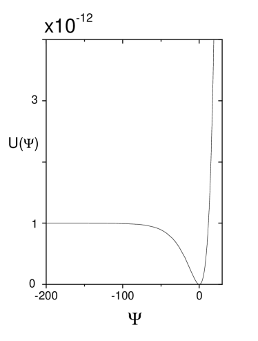
Figure 1: The plot shows an emergent scalar potential that allows for conventional reheating.

Potentials of this form have been considered previously, not only in the context of the emergent universe Ellis:2003qz ; Ellis:2002we ; Mulryne:2005ef but in a number of different settings, including cases that introduce higher-order curvature invariants into the Einstein-Hilbert action. Such corrections are required when attempting to renormalize theories of quantum gravity Antoniadis:1986tu . They also arise in low-energy limits of superstring theories Candelas:1985en . In general, these theories are conformally equivalent to Einstein gravity plus a minimally coupled, self-interacting scalar field. In particular, potentials with the structure of Eq. (28) can be obtained from theories that include a $R^{2}$ term in the action, where $R$ is the Ricci scalar Ellis:2003qz . In general, all these potentials possess a global minimum at $U=0$. Following Ref. Mulryne:2005ef , we take $U_{0}=10^{-12}$ and $\beta=0.1$ as representing typical values satisfying the constraints imposed by the WMAP satellite Peiris:2003ff ; Spergel:2003cb .

As an example of a Brans-Dicke potential that satisfies the condition of static solution, Eqs. (23) and (24), we consider the following polynomial potential

$$V(\Phi)=V_{0}+A\left(\Phi-\Phi_{0}\right)+\frac{1}{2}\,B\left(\Phi-\Phi_{0}\right)^{2}+\frac{1}{4!}\,\,C\left(\Phi-\Phi_{0}\right)^{4}\,,$$ (29)

where $\Phi_{0}$ correspond to the value of the JBD field at the static solution.

Following the discussion of Sect. IV, we choose the parameter $C$ in order to force $\Phi$ to settle down to a non-zero expectation value, $\Phi\rightarrow\Phi_{f}$. Then we have:

$$C=-12\left[\frac{2V_{0}-2A\,\Phi_{0}+B\,\Phi^{2}_{0}+A\,\Phi_{f}-B\,\Phi_{0}\,\Phi_{f}}{(\Phi_{0}-\Phi_{f})^{3}(\Phi_{0}+\Phi_{f})}\right].$$

The parameters $V_{0},A,B$ are fixed in order to obtain a static solution at $\Phi=\Phi_{0}$, $a=a_{0}$ and $\rho=\rho_{0}$

$$V_{0} = \frac{3\Phi_{0}}{a_{0}}-\rho_{0}\,,$$ (30)

$$A = \frac{3}{a_{0}^{2}}\,,$$ (31)

$$B = \frac{\chi}{2\,a^{2}_{0}\,\Phi_{0}}\,,$$ (32)

where we have introduced the dimensionless parameter $\chi$, satisfying $0<\chi<3/2$. The JBD parameter requires:

$$-\frac{3}{2}< w <-\frac{\sqrt{3}}{4}\,\sqrt{3-2\,\chi}-\frac{1}{4}(3+\chi)\,.$$ (33)

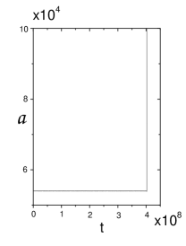
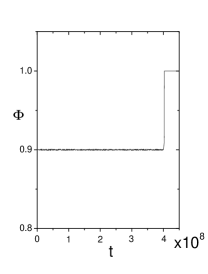
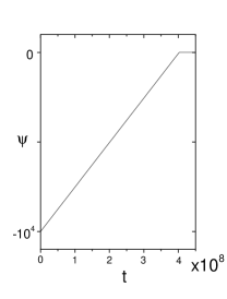
Figure 2: Behavior of the scale factor $a$, the JBD field $\Phi$ and the scalar field $\Psi$ as function of the cosmological time $t$.

The static energy density is given by:

$$\rho_{0}=\frac{\Phi_{0}}{a_{0}^{2}}+U_{0}\,.$$ (34)

In order to obtain a numerical solution we take the following values for the parameters in the JBD potential $\Phi_{0}=0.9$, $\Phi_{f}=1$, $a_{0}=5.4\times 10^{4}$, $\chi=1$ and $w=-1.45$, where we have used units in which $8\pi G=1$. These particular parameters satisfy all the constraints discussed previously. On the other hand, in order to consider the model just at the classical level we have to be out of the Planck era. This imposes the following conditions: $\rho<\Phi(t)^{2}$ and $V(\Phi)<\Phi(t)^{2}$, which are satisfied with the values of the parameters mentioned above.

Now, let us consider a numerical solution corresponding to a universe starting from an initial state close to the static solution. The whole evolution of the model is shown in Fig. (2), where we can notice that during the part of the process where the scalar field $\Psi$ moves in the asymptotically flat region of the potential $U(\Psi)$, the universe remains static, due to the form of the JBD potential, Eq. (29). This means that the scale factor and the JBD field do not evolve with the cosmological time keeping their equilibrium values $a_{0}$ and $\Phi_{0}$ during this period.

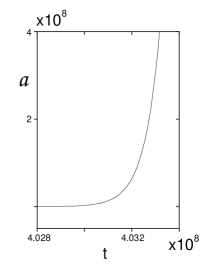
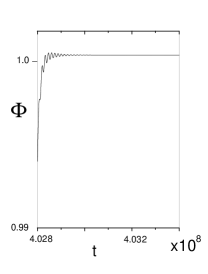
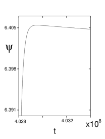
Figure 3: Plot showing $a$, $\Phi$ and $\Psi$ near the beginning of the inflationary period.

The static regimen finishes when the scalar field moves past the minimum of its potential (near the value $\Psi\sim 0$) and begins to decelerate as it moves up its potential. During this period the static equilibrium is broken, and the scale factor and with the JBD field start to evolve. Finally, the scalar field starts to go down the potential $U(\Psi)$ in the slow-roll regimen. The details of the last part of this process is shown in Fig (3), where we note that at the moment when the scalar field starts to roll back down its potential, the JBD field attains its quasi-static value $\Phi\sim 1$, and the scale factor starts its inflationary expansion.

On the other hand, a numerical solution corresponding to a universe starting from an initial state not in the static solution but close to it, presents small oscillations around the equilibrium values, as shown in Fig (4). This tells us that the static solution is stable.

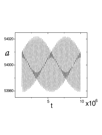
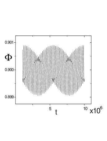
Figure 4: Graph showing the scale factor and the JBD field oscillating around their equilibrium values $a_{0}$ and $\Phi_{0}$, while the scalar field follows the constant potential.

VI Conclusions

In this paper we have studied a Jordan-Brans-Dicke model and we have determined whether that model could display the general characteristics required for an emergent universe scenario. That is a stable static past asymptotic solution followed by a period of de Sitter inflation.

The original idea of an emergent universe  Ellis:2002we is a simple closed inflationary model in which the universe emerges from an Einstein static state with radius $a_{0}>>L_{p}$, inflates and is then subsumed into a hot Big Bang era. The attractiveness of the proposed model is that one can avoid an initial quantum-gravity stage if the static radius is larger than the Planck length. However, this model suffers from the problem of instability of the Einstein static state (see Refs. Mulryne:2005ef ; Banerjee:2007qi ; Nunes:2005ra ; Lidsey:2006md ) which makes it extremely difficult to maintain its state for an infinitely long time in the presence of fluctuations, such as quantum fluctuations, thereby aborting the scenario.

In this work, we have provided an explicit construction of an emergent universe scenario, which presents a stable past eternal static solution and brings us the possibility of avoiding an initial quantum-gravity stage if we chose the static radius to be larger than the Planck length.

In particular, we have considered a JBD theory with a self interacting potential and matter content corresponding to a scalar field.

In the first part of the paper, we studied static solutions. In order to do so we determined the characteristics of the JBD potential and we took a constant scalar matter potential. In particular, we have found a static solution in which the JBD potential had a non-zero value and a positive derivative at the static point $\Phi=\Phi_{0}$. In determining the stability of this solution, we have calculated the real frequencies of small oscillation about the static solution. This imposed a bound for the first and second derivative of the JBD potential at the static point $0<V^{\prime\prime}_{0}<V^{\prime}_{0}/(2\Phi_{0})$. A restriction on the value of the JBD parameter $w$ was also obtained (see Eq. (24)). In this way, we have shown that it is possible to obtain a past eternal universe in a JBD model, depending upon the characteristics of the JBD potential and the Brans-Dicke parameter $w$.

In the second part of the paper, we studied the possibility that our model present a past eternal static solution, which eventually enters a phase where the stability of the static solution is broken by changing the matter scalar field potential, thereby leading to a phase of inflation.

In our model, the mechanism that enables the universe to emerge depends on the form of both potentials: the JBD potential $V(\phi)$ and the matter scalar field potential, $U(\Psi)$. For the scalar field potential it is required that it asymptotically approaches a constant value as $\Psi\rightarrow-\infty$, and in order to break the cycles it should grow in magnitude for larger $\Psi$. The JBD potential must satisfy similar requirements to that described in Ref. Green:1996xe .

In the third part of the paper, we studied a particular matter scalar potential, similar to the one used in the context of emergent universe Ellis:2003qz ; Ellis:2002we ; Mulryne:2005ef , and a polynomial JBD potential, which satisfies the requirement of static stable past eternal solution followed by a period of inflation, Eq (25).

We obtained numerical solutions for a universe starting from an initial state close to the static solution. The numerical solutions showed a behavior just like that discussed in previous sections. In particular we have found that when the scalar field $\Psi$ moves in the asymptotically flat region of the potential $U(\Psi)$, the scale factor and the JBD field experience small oscillations about their equilibrium points. After that, when the scalar field passes the minimum of its potential and begins to decelerate as it moves up its potential, we found that the static equilibrium is broken, and the scale factor and JBD field start to evolve. In particular, the numerical solution shows that when the scalar field starts to go down the potential $U(\Psi)$, the JBD field gets its quasi-static value and the scale factor begins a quasi-exponential expansion.

We should note that a more detailed analysis of this process could be done by using a dynamical system approach. We expect to return to this point in the near future.

- (1) Guth A., The inflationary universe: A possible solution to the horizon and flatness problems, 1981 Phys. Rev. D 23 347 .
- (2) Albrecht A. and Steinhardt P. J., Cosmology for grand unified theories with radiatively induced symmetry breaking, 1982 Phys. Rev. Lett. 48 1220.
- (3) Linde A. D., A new inflationary universe scenario: A possible solution of the horizon, flatness, homogeneity, isotropy and primordial monopole problems, 1982 Phys. Lett. 108B 389.
- (4) Linde A. D., Chaotic inflation, 1983 Phys. Lett. 129B 177.
- (5) Linde A. D., Particle physics and inflationary cosmology, arXiv:hep-th/0503203 (Harwood Academic Publishers, 1990).
- (6) Borde A. and Vilenkin A., Eternal inflation and the initial singularity, 1994 Phys. Rev. Lett. 72 3305.
- (7) Borde A. and Vilenkin A., Violation of the weak energy condition in inflating spacetimes, 1997 Phys. Rev. D 56 717.
- (8) Guth A. H., Eternal inflation, arXiv:astro-ph/0101507.
- (9) Borde A., Guth A. H. and Vilenkin A., Inflationary space-times are incompletein past directions, 2003 Phys. Rev. Lett. 90 151301.
- (10) Vilenkin A., Quantum cosmology and eternal inflation, arXiv:gr-qc/0204061.
- (11) Ellis G. F. R. and Maartens R., The emergent universe: Inflationary cosmology with no singularity, 2004 Class. Quant. Grav. 21 223.
- (12) Ellis G. F. R., Murugan J. and Tsagas C. G., The emergent universe: An explicit construction, 2004 Class. Quant. Grav. 21 233.
- (13) Mulryne D. J., Tavakol R., Lidsey J. E. and Ellis G. F. R., An emergent universe from a loop, 2005 Phys. Rev. D 71 123512.
- (14) Mukherjee S., Paul B. C., Maharaj S. D. and Beesham A., Emergent universe in Starobinsky model, arXiv:gr-qc/0505103.
- (15) Mukherjee S., Paul B. C., Dadhich N. K., Maharaj S. D. and Beesham A. , Emergent universe with exotic matter, 2006 Class. Quant. Grav. 23 6927.
- (16) Banerjee A., Bandyopadhyay T. and Chakraborty S., Emergent universe in brane world scenario, arXiv:0705.3933 [gr-qc].
- (17) Nunes N. J., Inflation: A graceful entrance from loop quantum cosmology, 2005 Phys. Rev. D 72 103510.
- (18) Lidsey J. E. and Mulryne D. J., A graceful entrance to braneworld inflation, 2006 Phys. Rev. D 73 083508.
- (19) Gibbons G. W., The entropy and stability of the universe, 1987 Nucl. Phys. B 292 784 .
- (20) Gibbons G. W., Sobolev’s inequality, Jensen’s theorem and the mass and entropy of the universe, 1988 Nucl. Phys. B 310 636.
- (21) Jordan P., The present state of Dirac’s cosmological hypothesis, 1959 Z.Phys. 157 112; Brans C. and Dicke R. H., Mach’s principle and a relativistic theory of gravitation, 1961 Phys. Rev. 124 925.
- (22) Freund P. G. O., Kaluza-Klein cosmologies, 1982 Nucl. Phys. B 209 146.
- (23) Appelquist T., Chodos A. and Freund P. G. O., Modern Kaluza-Klein theories ( 1987 Addison-Wesley, Redwood City).
- (24) Fradkin E. S. and Tseytlin A. A., Effective field theory from quantized strings, 1985 Phys. Lett. B 158 316.
- (25) Fradkin E. S. and Tseytlin A. A., Quantum string theory effective action, 1985 Nucl. Phys. B 261 1.
- (26) Callan C. G., Martinec E. J., Perry M. J. and Friedan D., Strings in background fields, 1985 Nucl. Phys. B 262 593.
- (27) CallanC. G., Klebanov I. R. and Perry M. J. , String theory effective actions, 1986 Nucl. Phys. B 278 78.
- (28) Green M. B., Schwarz J. H. and Witten E., Superstring theory (1987 Cambridge, Uk: Univ. Pr., Cambridge Monographs On Mathematical Physics).
- (29) La D., Steinhardt P. J. and Bertschinger E. W. , Prescription for successful extended inflation, 1989 Phys. Lett. B 231 231 .
- (30) Bertolami O. and Martins P. J. , Non-minimal coupling and quintessence, 2000 Phys. Rev. D 61 064007.
- (31) Banerjee N. and Pavon D., Cosmic acceleration without quintessence, 2001 Phys. Rev. D 63 043504.
- (32) Sen A. A. and Sen S., Cosmology in scalar tensor theory and asymptotically de-Sitter universe, 2001 Mod. Phys. Lett. A 16 1303.
- (33) Green A. M. and Liddle A. R., Open inflationary universes in the induced gravity theory, 1997 Phys. Rev. D 55 609.
- (34) Antoniadis I. and Tomboulis E. T., Gauge invariance and unitarity in higher derivative quantum gravity, 1986 Phys. Rev. D 33 2756.
- (35) Candelas P., Horowitz G. T., Strominger A. and Witten E., Vacuum configurations for superstrings, 1985 Nucl. Phys. B 258 46 .
- (36) Peiris H. V. et al. [WMAP Collaboration], First year Wilkinson Microwave Anisotropy Probe (WMAP) observations: Implications for inflation, 2003 Astrophys. J. Suppl. 148 213.
- (37) Spergel D. N. et al. [WMAP Collaboration], First Year Wilkinson Microwave Anisotropy Probe (WMAP) Observations: Determination of cosmological parameters, 2003 Astrophys. J. Suppl. 148 175.