On the recognition of fundamental physical principles in recent atmospheric-environmental studies

Abstract

In this paper, so-called alternative mass balance equations for atmospheric constituents published recently are assessed in comparison with the true local mass balance equations deduced from exact integral formulations. It is shown that these alternative expressions appreciably violate the physical law of the conservation of mass as expressed by the equation of continuity. It is also shown that terms of these alternative mass balance equations have different physical units, a clear indication that these alternative expressions are incorrect. Furthermore, it is argued that in the case of alternative mass balance equations a real basis for Monin-Obukhov similarity laws does not exist. These similarity laws are customarily used to determine the turbulent fluxes of momentum, sensible heat and matter in the so-called atmospheric surface layer over even terrain. Moreover, based on exact integral formulations a globally averaged mass balance equation for trace species is derived. It is applied to discuss the budget of carbon dioxide on the basis of the globally averaged natural and anthropogenic emissions and the globally averaged uptake caused by the terrestrial biosphere and the oceans.

1 Introduction

Recently, Finnigan et al. [15] and many others [2, 14, 16, 17, 39, 40, 42, 44, 62] proposed alternative forms of balance equations of atmospheric constituents. Unfortunately, these equations are not self-consistent and their terms are afflicted with different physical units. The latter is a clear indication that something is going wrong. Since mainly the results of turbulent fluxes of carbon dioxide ($CO_{2}$) published recently were harmfully affected by these alternative mass balance equations, these results must be assessed carefully, especially in front of the debate on global warming due to an increase of greenhouse gases like $CO_{2}$.
To assess these alternative mass balance equations it is indispensable to compare them with the correct ones. Therefore, in section 2 we will derive the correct local mass balance equations from exact integral mass balance equations and discuss them physically. It is shown in section 3 that one of the fundamental physical principles namely the conservation of mass (as expressed by the equation of continuity) is notably violated by the alternative mass balance equations. Some aspects of Reynolds averaging are briefly, but thoroughly discussed in section 4. In identifying an adequate averaging time, we argue that the Allan variance criterion [1] combined with the wavelet analysis is much more favorable than block averaging as suggested, for instance, by Finnigan et al. [15] and Trevi o and Andreas [68]. In section 5, we present the Reynolds averaged mass balance equations for a turbulent fluid and compare it with that of the alternative forms. In section 6, these different forms of mass balance equations are vertically integrated by assuming horizontal homogeneity and the results obtained are assessed. We show in section 7 that in the case of the alternative form of the mass balance equations a real basis for Monin-Obukhov similarity laws does not exist. Consequently, such similarity laws customarily used for determining the flux densities (hereafter, a flux density is simply called a flux) of long-lived trace gases like $CO_{2}$ would be obsolete. Based on exact integral formulations a globally averaged mass balance equation for trace species is derived in section 8 to underline that the emission and uptake of matter serve as boundary conditions. This result is in complete contrast to the alternative mass balance equation in which emission and uptake are considered as volume-related source/sink functions. Final remarks and our conclusions are listed in section 9.

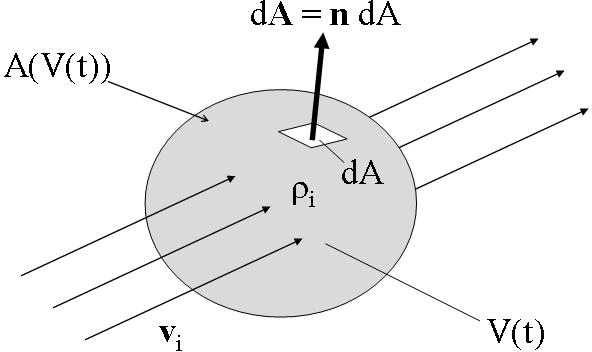
Figure 1: Transfer of matter through the surface $A(V(t))$ of a given volume $V(t)$.

2 The mass balance equations of atmospheric constituents for a macroscopic fluid

First, we will derive the conservation laws for a macroscopic fluid (often called a molecular flow). The total rate of change in the mass $M_{i}$ of a constituent, $i=0,1,\dots,N$, within an arbitrary volume $V(t)$ that also depends on time, $t$, can be expressed by [10]

$$\frac{dM_{i}}{dt}=\frac{d}{dt}\int_{V(t)}\rho_{i}\;dV\;,$$ (1)

where $\rho_{i}=M_{i}/V$ is the corresponding partial density. This quantity $dM_{i}/dt$ is equal to the material flow of the $i^{th}$ component into and out of this volume through its surface $A(V(t))$, i.e., the exchange of material between the volume and its surroundings, and the net production/depletion $\sigma_{i}=f(\rho_{1},\dots,\rho_{N})$ of the $i^{th}$ constituent per unit volume owing to chemical reactions (and phase transition effects) that occur inside $V$. Thus, we have (see Figure 1)

$$\frac{d}{dt}\int_{V(t)}\rho_{i}\;dV=-\int_{A(V(t))}\rho_{i}\;\textbf{v}_{N}\cdot d\textbf{A}+\int_{V(t)}\sigma_{i}\;dV\;.$$ (2)

Here, $\textbf{v}_{N}=\textbf{v}_{i}-\textbf{v}$ is the net velocity that characterizes the diffusion of the $i^{th}$ constituent with respect to the barycentric flow, considered as being of Newtonian kind. The quantity $\textbf{v}_{i}$ is the individual velocity, and v denotes the barycentric velocity defined by

$$\textbf{v}=\frac{1}{\rho}\sum_{i=0}^{N}\rho_{i}\;\textbf{v}_{i}\;,$$ (3)

where

$$\rho=\frac{M}{V}=\frac{1}{V}\sum_{i=0}^{N}M_{i}=\sum_{i=0}^{N}\rho_{i}$$ (4)

is the total density of air. The use of the barycentric velocity as a reference velocity, of course, is not the only possibility to describe diffusion. Prigogine [57] deduced from the entropy principle that in systems with mechanical equilibrium diffusion processes can be related to an arbitrary reference velocity. Herbert [23, 24] discussed the general application of Prigogine’s diffusion theorem to the atmosphere and some specific invariance properties of the thermodynamic laws as well as various alternative relations to describe Fick-type mass diffusion in a (diluted) binary gas mixture such as the atmosphere. Nevertheless, in our contribution the diffusion is related to the barycentric velocity and the quantity $\textbf{J}_{i}=\rho_{i}\textbf{v}_{N}=\rho_{i}(\textbf{v}_{i}-\textbf{v})$ is denoted as the diffusion flux of the $i^{th}$ constituent. Furthermore, $d\textbf{A}=\textbf{n}\;dA$ is a vector normal to the surface of the volume $V$ with the unit vector n and the magnitude $dA$. The unit vector is counted positive from inside to outside of the volume. Note that $i=0$ denotes that portion of dry air which is chemically inert, i.e., this portion does not contain any chemically active atmospheric constituent. Furthermore, the occurrence of the surface integral in Eq. (2) means that we consider a system that is open in the sense of thermodynamics, when the exchange of energy is allowed, too. It is the most general one.
Since the volume is considered as time-dependent, the differentiation of the volume with respect to time is also required. It can be performed by applying Leibnitz’s integral theorem. In doing so, we obtain for the total rate of change, $dM_{i}/dt$,

$$\frac{d}{dt}\int_{V(t)}\rho_{i}\;dV=\int_{V(t)}\frac{\partial{\rho_{i}}}{\partial{t}}\;dV+\int_{A(V(t))}\rho_{i}\;\textbf{v}\cdot d\textbf{A}\;.$$ (5)

Thus, combining equations (2) and (5) results in

$$\frac{d}{dt}\int_{V(t)}\rho_{i}\;dV = \int_{V(t)}\frac{\partial{\rho_{i}}}{\partial{t}}\;dV+\int_{A(V(t))}\rho_{i}\;\textbf{v}\cdot d\textbf{A}$$ (6)

$$= -\int_{A(V(t))}\textbf{J}_{i}\cdot d\textbf{A}+\int_{V(t)}\sigma_{i}\;dV$$

or

$$\int_{V(t)}\frac{\partial{\rho_{i}}}{\partial{t}}\;dV+\int_{A(V(t))}\bigl{(}\rho_{i}\;\textbf{v}+\textbf{J}_{i}\bigr{)}\cdot d\textbf{A}=\int_{V(t)}\sigma_{i}\;dV\;.$$ (7)

This expression is called the integral balance equation of the $i^{th}$ atmospheric constituent. It is a very general formulation and not affected by any kind of averaging process usually applied in deriving local balance equations for turbulent systems like the atmospheric boundary layer. McRae and Russell [45], for instance, used such an integral formulation for practical purposes by considering the domain of the South Coast Air Basin of Southern California.
By applying Gauss’ integral theorem (often called the divergence theorem), the surface integral occurring in Eq. (7) can by replaced by a volume integral so that we obtain

$$\int_{V(t)}\frac{\partial{\rho_{i}}}{\partial{t}}\;dV+\int_{V(t)}\nabla\cdot\bigl{(}\rho_{i}\;\textbf{v}+\textbf{J}_{i}\bigr{)}\;dV=\int_{V(t)}\sigma_{i}\;dV\;,$$ (8)

where $\nabla$ is the nabla (or del) operator. Since in Eq. (8) the shape of the volume is arbitrary, we may also write:

$$\frac{\partial{\rho_{i}}}{\partial{t}}+\nabla\cdot\bigl{(}\rho_{i}\;\textbf{v}+\textbf{J}_{i}\bigr{)}=\sigma_{i}\;.$$ (9)

This equation is called the local balance equation of the $i^{th}$ constituent [9, 10, 32, 58, 61, 64]. The term $\partial{\rho_{i}}/\partial{t}$ is the local temporal change of $\rho_{i}$, and the quantities $\rho_{i}\textbf{v}$ and $\textbf{J}_{i}$ are frequently called the convective and non-convective transports of matter, respectively. It is obvious that in the case of a closed or isolated thermodynamic system the divergence term vanishes because it only describes the exchange of matter between the system and its surroundings. As the use of Gauss’ integral theorem requires that some mathematical pre-requisites have to be fulfilled, the local balance equation (9) is somewhat lesser valid than the integral balance equation (7). Nevertheless, any integration of Eq. (9) over a certain volume as performed, for instance, by numerical models of the troposphere must be in agreement with Eq. (7).
Summing Eq. (9) over all substances, $i=0,1.\dots,N$, provides

$$\sum_{i=0}^{N}\frac{\partial{\rho_{i}}}{\partial{t}}+\sum_{i=0}^{N}\nabla\cdot\bigl{(}\rho_{i}\;\textbf{v}+\textbf{J}_{i}\bigr{)}=\sum_{i=0}^{N}\sigma_{i}\;.$$ (10)

Since, according to de Lavoisier’s law, mass is conserved in chemical reactions (and/or phase transition processes; i.e., the transformation of mass into energy as expressed by Einstein’s formula is unimportant in the case of atmospheric trace constituents), we have

$$\sum_{i=0}^{N}\sigma_{i}=0\;.$$ (11)

Furthermore, with the aid of Eqs. (3) and (4) and the definition of the diffusion flux, we obtain

$$\sum_{i=0}^{N}\frac{\partial{\rho_{i}}}{\partial{t}}=\frac{\partial{}}{\partial{t}}\Bigl{(}\sum_{i=0}^{N}\rho_{i}\Bigr{)}=\frac{\partial{\rho}}{\partial{t}}$$ (12)

and

$$\sum_{i=0}^{N}\nabla\cdot(\rho_{i}\;\textbf{v}+\textbf{J}_{i}) = \nabla\cdot\Bigl{(}\sum_{i=0}^{N}\bigl{(}\rho_{i}\;\textbf{v}+\rho_{i}(\textbf{v}_{i}-\textbf{v})\bigr{)}\Bigr{)}$$ (13)

$$= \nabla\cdot\Bigl{(}\sum_{i=0}^{N}\bigl{(}\rho_{i}\;\textbf{v}_{i}\bigr{)}\Bigr{)}=\nabla\cdot\bigl{(}\rho\;\textbf{v}\bigr{)}\;.$$

Thus, Eq, (10) leads to the macroscopic balance equation for the total mass per unit volume [10, 20, 32, 37, 58, 64]

$$\frac{\partial{\rho}}{\partial{t}}+\nabla\cdot\bigl{(}\rho\;\textbf{v}\bigr{)}=0\;.$$ (14)

It represents the formulation of the conservation of mass on the local scale and is customarily called the equation of continuity.
If we use the mass fraction $c_{i}=\rho_{i}/\rho$, then Eq. (9) will read

$$\frac{\partial{\bigl{(}\rho\;c_{i}\bigr{)}}}{\partial{t}}+\nabla\cdot\bigl{(}\rho\;c_{i}\;\textbf{v}+\textbf{J}_{i}\bigr{)}=\sigma_{i}\;.$$ (15)

Applying the product rule of differentiation to this equation yields

$$\rho\;\frac{\partial{c_{i}}}{\partial{t}}+c_{i}\Bigl{(}\underbrace{\frac{\partial{\rho}}{\partial{t}}+\nabla\cdot\bigl{(}\rho\;\textbf{v}\bigr{)}}_{=\;0\;(seeEq.(\ref{2.14}))}\Bigr{)}+\rho\;\textbf{v}\cdot\nabla{c_{i}}+\nabla\cdot\textbf{J}_{i}=\sigma_{i}$$ (16)

or

$$\rho\Bigl{(}\frac{\partial{c_{i}}}{\partial{t}}+\textbf{v}\cdot\nabla{c_{i}}\Bigr{)}+\nabla\cdot\textbf{J}_{i}=\sigma_{i}\;,$$ (17)

where

$$\frac{dc_{i}}{dt}=\frac{\partial{c_{i}}}{\partial{t}}+\textbf{v}\cdot\nabla{c_{i}}$$ (18)

is the substantial or total derivative with respect to time. Equation (17) may be called the advection-diffusion equation of a chemically active atmospheric constituent.

3 The alternative mass balance equations of atmospheric constituents

Recently, several authors proposed a mass balance as an alternative form to the conservation equation (9). This alternative form reads [2, 14, 15, 16, 17, 39, 40, 42, 44, 62]

$$\frac{\partial{\rho_{i}}}{\partial{t}}+\nabla\cdot\bigl{(}\rho_{i}\;\textbf{v}\bigr{)}=S_{i}\;.$$ (19)

In this equation, the diffusion flux $\textbf{J}_{i}$ is generally ignored. This flux, however, is not negligible because, as expressed in Eq. (9), it must represent the local balance equation for a macroscopic fluid. If $\textbf{J}_{i}$ would not occur, diffusion of the $i^{th}$ constituent in a macroscopic fluid could not be quantified. This means, for instance, that the sedimentation of airborne particles like aerosol and ice particles and water drops would generally be excluded. Moreover, this alternative form is applied to quantify the sinks or sources of $CO_{2}$ inside canopies of tall vegetation like forests by a method where the term $S_{i}$ is called a source/sink inside the volume $V$ of the fluid. However, considering the derivation of Eq. (9), an uptake or emission of a substance by plant elements or soil is a process at the boundary of a fluid and, therefore, has to be described in terms of boundary conditions, as substantiated by the integral balance equation (7). Therefore, $S_{i}$ is not a biological source/sink term. Such a term must not occur in the local form of a balance equation. Boundary conditions only occur when the local mass balance equation is integrated, in complete agreement with Eq. (7). The alternative equation (19), however, cannot be deduced from any integral mass balance equation. Finnigan et al. [15] introduced it into the literature in an unforced manner and without any physical justification. One of the physical consequences related to this alternative mass balance equation is that the biological source/sink would explicitly cause a temporal change in the partial density. Whereas Eq. (9) clearly substantiates that only the divergence of the convective and non-convective fluxes contributes to a temporal change of the partial density.
Finnigan et al. [15] and many others [2, 14, 16, 17, 39, 40, 42, 44, 62] expressed $S_{i}$ as a surface source (instead of a volume-related source or sink due to chemical reactions or/and phase transition processes) by

$$S_{i}=S_{i}\bigl{(}\textbf{x}\bigr{)}\;\delta\bigl{(}\textbf{x}-\textbf{x}_{0}\bigr{)}\;,$$ (20)

where $\delta(\textbf{x}-\textbf{x}_{0})$ is Dirac’s delta function (from a mathematical point of view a distribution). Finnigan et al. [15] argued that the source term, $S_{i}(\textbf{x})$, is multiplied by the Dirac delta function, signifying that the source is zero except on the ground and vegetation surfaces, whose locus is $\textbf{x}_{0}$ . This is incorrect at least by two reasons: As mentioned before, the physical meaning of $S_{i}$ in Eq.(19) must be a source or sink within the volume, but not at the boundaries, which are represented by boundary conditions. Furthermore, the Dirac delta function has the property that $\delta(\textbf{x}-\textbf{x}_{0})=0$ for all $\textbf{x}\neq\textbf{x}_{0}$ [5, 11, 38, 46, 59], i.e., there is only the infinitesimal region (namely when $\textbf{x}=\textbf{x}_{0}$) at which a source or sink of matter is defined. In addition, in various textbooks [38, 46], it is pointed out that $\delta(\textbf{x}-\textbf{x}_{0})=\infty$ for $\textbf{x}=\textbf{x}_{0}$. Thus, Eq. (20) and, hence, Eq. (19) would become meaningless for $\textbf{x}=\textbf{x}_{0}$. As pointed out later on, the main properties of the $\delta$-function are defined by the integral over a region containing $\textbf{x}=\textbf{x}_{0}$.
Uptake and emission of a constituent by plants, soil and/or water systems are surface effects, expressed, for instance, in SI units by $kg/(m^{2}s)$; whereas the local temporal change in Eqs. (9) and (15) has the SI units $kg/(m^{3}s)$. If we express Dirac’s delta function using SI units we will have $m^{-3}$. Therefore, the term $S_{i}(\textbf{x})\;\delta(\textbf{x}-\textbf{x}_{0})$ would have the SI units $kg/(m^{5}s)$. It is indispensable that in any physical equation its terms must have identical physical units. This fundamental requirement, however, is not satisfied in the case of the alternative forms of mass balance equations. There is evidence (e.g., Eq. (6) of Finnigan et al. [15], Eq. (11) of Finnigan [16], Eqs. (2.2) and (3.8) of Lee et al. [40], and Eq. (14) of Massman and Tuovinen [44]) that the biological source/sink term is, indeed, expressed by the units of a flux of matter, i.e., in $kg/(m^{2}s)$, even though, as expressed by the local temporal change of the partial density ($\partial{\rho_{i}}/\partial{t}$), $kg/(m^{3}s)$ is unequivocally required.
Nevertheless, assuming for a moment that Eq. (20) is reasonable, then Eq. (11) would result in

$$\sum_{i=1}^{N}S_{i}=\sum_{i=1}^{N}S_{i}\bigl{(}\textbf{x}\bigr{)}\;\delta\bigl{(}\textbf{x}-\textbf{x}_{0}\bigr{)}\neq 0\;,$$ (21)

and, hence, Eq. (10) in

$$\frac{\partial{\rho}}{\partial{t}}+\nabla\cdot\bigl{(}\rho\;\textbf{v}\bigr{)}=\sum_{i=1}^{N}S_{i}\bigl{(}\textbf{x}\bigr{)}\;\delta\bigl{(}\textbf{x}-\textbf{x}_{0}\bigr{)}\neq 0\;.$$ (22)

The right-hand side of this equation is not equal to zero because atmospheric constituents have different natural and anthropogenic origins and different sinks. This means: if Eq. (20) would be reasonable, than one of the fundamental laws of physics, namely the conservation of the total mass on a local scale, as expressed by the equation of continuity (14), is notably violated by the alternative forms of mass balance equations.

4 Reynolds averaging calculus

Conservation laws for a turbulent fluid can be derived by using Reynolds’ averaging calculus, i.e., decomposition of any instantaneous field quantity $\varphi(\textbf{r})$ like $\rho_{i}(\textbf{r})$ and $\textbf{v}(\textbf{r})$ by $\varphi(\textbf{r})=\overline{\varphi}+\varphi^{\prime}$ and subsequent averaging according to [22, 32, 69]

$$\overline{\varphi}=\overline{\varphi(\textbf{r})}=\frac{1}{G}\int_{G}\varphi\bigl{(}\textbf{r},\textbf{r}^{\prime}\bigr{)}\;dG^{\prime}\;,$$ (23)

where $\overline{\varphi}$ is the average in space and time of $\varphi(\textbf{r})$, and the fluctuation $\varphi^{\prime}$ is the difference between the former and the latter. Here, r is the four-dimensional vector of space and time in the original coordinate system, $\textbf{r}^{\prime}$ is that of the averaging domain $G$ where its origin, $\textbf{r}^{\prime}=0$, is assumed to be r, and $dG^{\prime}=d^{3}r\;dt^{\prime}$. The averaging domain $G$ is given by $G=\int_{G}dG^{\prime}$. Hence, the quantity $\overline{\varphi}$ represents the mean values for the averaging domain $G$ at the location r. Since $\overline{\overline{\varphi}}=\overline{\varphi}$, averaging the quantity $\varphi(\textbf{r})=\overline{\varphi}+\varphi^{\prime}$ provides $\overline{\varphi^{\prime}}=0$. Any kind of averaging must be in agreement with these basic definitions. These basic definitions cannot be undermined by imperfect averaging procedures. Since, in accord with the ergodic theorem, assemble averaging as expressed by Eq. (23) may be replaced by time averaging [41], the common practice, it is indispensable to ask whether a time averaging procedure is in complete agreement with the statistical description of turbulence or not.
A basic requirement for using a time averaging procedure is that turbulence is statistically steady [13, 43, 67]. Consequently, sophisticated procedures for identifying non-stationary effects (trends) are indispensable to prevent that computed turbulent fluxes of atmospheric constituents are notably affected by non-stationary effects. In order to identify such stationary states in the off-line time series analysis, Werle et al. [70] suggested the Allan-variance criterion [1] as a suitable and efficient tool. As argued by Percival and Guttorp [54], this variance is an appropriate measure for studying long-memory processes because it can be estimated without bias and with good efficiency for such processes, and it may be interpreted as the Haar wavelet coefficient variance [18, 31]. Percival and Guttorp [54] generalized this to other wavelets [36]. Following various authors [6, 21, 26, 28], wavelet decomposition seems to be well appropriate to study turbulence data. Thus, the Allan variance criterion combined with the wavelet analysis is much more favorable than simple block averaging as suggested, for instance, by Finnigan et al. [15] and Trevi o and Andreas [68].

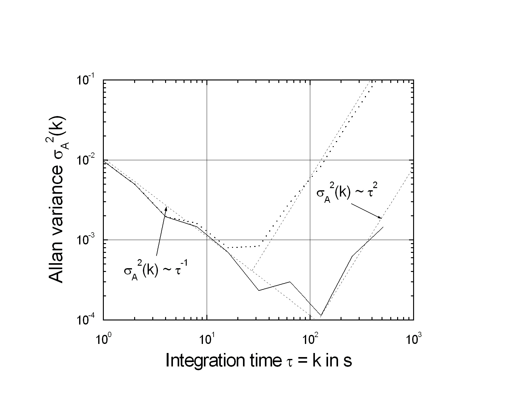
Figure 2: Allan plots deduced from the time series data illustrated in Figure 3 (solid line) and a data set which differs from that by a ten times stronger drift (dotted line). The dashed lines indicate white noise ($\tau^{-1}$) and linear drift ($\tau^{2}$) behavior (adopted from [31]).

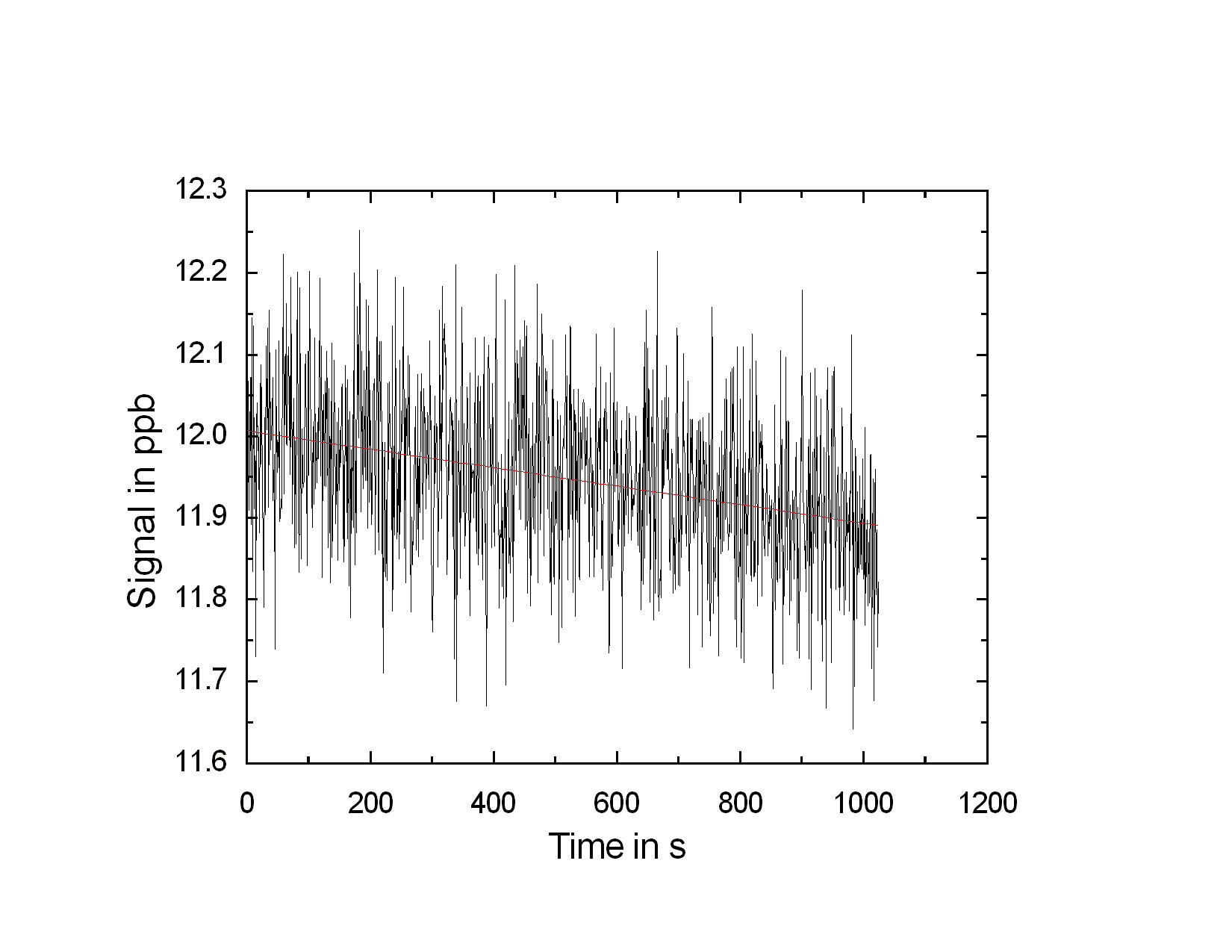
Figure 3: Generated time series data of a concentration consisting of an offset, a linear drift and a Gaussian distributed white noise. The sample size amounts to $N=2^{10}=1024$ (adopted from [71]).

Figure 2 illustrates two Allan plots deduced from a synthetic data set generated by the equation $Y_{t}=a+b\;t+G(\sigma)$ (see Figure 3), where $a$ is an offset, $b\;t$ is a linear drift and $G(\sigma)$ is a Gaussian distributed white noise (lower trace) and a data set containing a ten times stronger drift (upper trace). In both cases $\sigma_{A}^{2}(k)$ was calculated using Haar wavelet coefficients [31]. For convenience, it is assumed that the sampling interval between consecutive observations is constant and amounts to $\Delta{t}=1\;s$. Thus, the time $\tau=k\;\Delta{t}$ is equivalent to the averaging or integration time. As shown in Figure 3, the lower trace indicates a minimum of $\sigma_{A}^{2}(k)$ at an integration time, denoted here as optimum integration time $\tau_{opt}$, of about $130\;s$. Whereas the upper trace for the data set with the ten times stronger drift suggests a $\tau_{opt}$ value of about $25\;s$. For $\tau<\tau_{opt}$, the Allan plots show a $\tau^{-1}$ behavior that is typical for white noise. Beyond $\tau_{opt}$, the Allan plots obey the $\tau^{2}$ law which indicates that a linear drift becomes dominant. Consequently, for $\tau>\tau_{opt}$, stationary conditions as required by time averaging are not assured. From this point of view, $\tau_{opt}$ may be considered as the maximum averaging time [31].

5 The balance equations of atmospheric constituents for a turbulent fluid

Applying the conventional Reynolds’ averaging calculus to Eq. (9) yields [9, 32]

$$\frac{\partial{\overline{\rho_{i}}}}{\partial{t}}+\nabla\cdot\Bigl{(}\overline{\rho_{i}}\;\overline{\textbf{v}}+\overline{\rho_{i}^{\prime}\;\textbf{v}^{\prime}}+\overline{\textbf{J}_{i}}\Bigr{)}=\overline{\sigma_{i}}\;.$$ (24)

Here, the overbar represents the conventional Reynolds average; whereas the prime denotes the departure from that. Equation (24) is called the balance equation for the $1^{st}$ moment (or $1^{st}$-order balance equation). Here, $\overline{\rho_{i}^{\prime}\;\textbf{v}^{\prime}}$ is the turbulent (or eddy) flux. It is a non-convective flux, too.
As mentioned before, the diffusion flux represents not only molecular fluxes, but also the sedimentation of aerosol particles affected by the gravity field. Thus, $\overline{\textbf{J}_{i}}$ cannot generally be neglected in comparison with the corresponding second moment $\overline{\rho_{i}^{\prime}\;\textbf{v}^{\prime}}$. Even in the immediate vicinity of the earth’s surface it must not be ignored because the wind vector vanishes at any rigid surface, and, consequently, no exhalation or deposition of matter would be possible. In the case of gaseous constituents $\overline{\textbf{J}_{i}}$ becomes negligible in comparison with $\overline{\rho_{i}^{\prime}\;\textbf{v}^{\prime}}$ when a fully turbulent flow is considered. Obviously, Eq. (24) also fulfils the conditions $\sum_{i=0}^{N}\overline{\textbf{J}_{i}}=0$ and $\sum_{i=1}^{N}\overline{\sigma_{i}}=0$, and, as required by the equation of continuity in its averaged form,

$$\frac{\partial{\overline{\rho}}}{\partial{t}}+\nabla\cdot\Bigl{(}\overline{\rho}\;\overline{\textbf{v}}+\overline{\rho^{\prime}\;\textbf{v}^{\prime}}\Bigr{)}=0\;,$$ (25)

the conditions $\sum_{i=0}^{N}\overline{\rho_{i}}\;\overline{\textbf{v}}=\overline{\rho}\;\overline{\textbf{v}}$ and $\sum_{i=0}^{N}\overline{\rho_{i}^{\prime}\;\textbf{v}^{\prime}}=\overline{\rho^{\prime}\;\textbf{v}^{\prime}}$ are fulfilled, too.
If mass fractions are considered (see Eqs. (15) to (18)), then density-weighted averaging techniques [12, 22, 30, 55, 69] should be applied in formulating local balance equations for turbulent flows to avoid any simplification [32, 34].
If we rearrange Eq. (24) by using the equation of continuity (25) (it is similar to the rearrangement of Eq. (15) that leads to Eq. (17)) and ignoring the covariance terms $\overline{\rho^{\prime}\;\textbf{v}^{\prime}}$ and $\overline{\rho^{\prime}\;c_{i}^{\prime}}$, as customarily accepted within the framework of the Boussinesq approximation, we will obtain

$$\overline{\rho}\Bigl{(}\frac{\partial{\overline{c_{i}}}}{\partial{t}}+\overline{\textbf{v}}\cdot\nabla{\overline{c_{i}}}\Bigr{)}+\nabla\cdot\Bigl{(}\overline{\rho_{i}^{\prime}\;\textbf{v}^{\prime}}+\overline{\textbf{J}_{i}}\Bigr{)}=\overline{\sigma_{i}}\;.$$ (26)

It may be called the advection-diffusion equation of a chemically active atmospheric constituent for a turbulent fluid. Here, $\sigma_{i}$ still represents the gain or lost of matter due to chemical reactions (and/or phase transition processes).
For the purpose of comparison: Finnigan’s [16] Eqs. (8) as well as Eq. (3.7) and (10.8) of Lee et al. [40] read

$$\frac{\partial{\overline{\rho_{i}}}}{\partial{t}}+\overline{\textbf{v}}\cdot\nabla{\overline{\rho_{i}}}+\nabla\cdot\Bigl{(}\overline{\rho_{i}^{\prime}\;\textbf{v}^{\prime}}\Bigr{)}=\overline{S_{i}}\;,$$ (27)

where $S_{i}$ is still given by $S_{i}(\textbf{x})\delta(\textbf{x}-\textbf{x}_{0})$ (see our Eq. (20)). Obviously, Eq. (27) is not self-consistent. First, as shown in Eq. (26), the mass fraction $c_{i}$ must occur in the two terms on the left-hand side of Eq. (27), but not the partial density $\rho_{i}$. Second, the rearrangement of Eq. (15) that leads to Eq. (17) requires that the right-hand side of Eq. (22) is always equal to zero so that Eq. (22) equals the equation of continuity (14).

6 Vertically integrated mass balance equations

If we assume horizontally homogeneous conditions and recognize that in such a case the vertical component of the mean wind vector becomes nearly equal to zero ($\overline{w}\cong 0$), Eq. (24) will provide

$$\frac{\partial{\overline{\rho_{i}}}}{\partial{t}}+\frac{\partial}{\partial{z}}\Bigl{(}\overline{\rho_{i}^{\prime}\;w^{\prime}}+\overline{J_{i,z}}\Bigr{)}=\overline{\sigma_{i}}\;,$$ (28)

where, $w$ is the vertical component of the wind vector, $J_{i,z}$ is the vertical component of the diffusion flux, and $z$ is the height above ground. Note that Archimedean effects are related to the gravity field. The same is true in the case of the hydrostatic pressure. Consequently, the vertical direction is related to the gravity field[65]; but not to the normal vector of a slope or a streamline as recently described, for instance, by Finnigan et al. [15] and Finnigan [16]. Especially over complex terrain trajectories and streamlines are usually vary with time and position. Therefore, it is difficult to find, for instance, a common reference streamline coordinate frame for using sonic anemometry at different heights to estimate the variation of turbulent fluxes of momentum, sensible heat and matter with height. Without knowing a reference coordinate frame that is invariant in space and time, the convergence/divergence of any trace gases cannot be calculated [65, 66]. In contrast to a streamline coordinate frame, one may use a terrain-following coordinate frame as usually considered within the framework of mesoscale meteorological modeling, but an exact transformation of the governing equations is still indispensable. Fortunately, this transformation is well known since more than three decades (see, e.g., [56]).
The integration of this equation from the earth’s surface ($z=0$) to a certain height above ground ($z=h$),where a fully turbulent flow is established, yields then

$$\int_{0}^{h}\Bigl{(}\frac{\partial{\overline{\rho_{i}}}}{\partial{t}}-\overline{\sigma_{i}}\Bigr{)}dz=\Bigl{[}\overline{\rho_{i}^{\prime}\;w^{\prime}}+\overline{J_{i,z}}\Bigr{]}_{z=0}-\Bigl{[}\overline{\rho_{i}^{\prime}\;w^{\prime}}+\overline{J_{i,z}}\Bigr{]}_{z=h}\quad.$$ (29)

Assuming long-lived trace species ($\overline{\sigma_{i}}\cong 0$) and stationary condition ($\partial{\overline{\rho_{i}}}/\partial{t}=0$)leads to the constant flux approximation expressed by

$$\Bigl{[}\overline{\rho_{i}^{\prime}\;w^{\prime}}+\overline{J_{i,z}}\Bigr{]}_{z=h}=\Bigl{[}\overline{\rho_{i}^{\prime}\;w^{\prime}}+\overline{J_{i,z}}\Bigr{]}_{z=0}\;.$$ (30)

At the height $z=h$ the vertical component of the diffusion flux of a trace gas can usually be ignored in comparison with the vertical component of the corresponding eddy flux component ($|\overline{J_{i,z}}|_{z=h}\ll|\overline{\rho_{i}^{\prime}\;w^{\prime}}|_{z=h}$). As already mentioned, the opposite is true in the immediate vicinity of the earth’s surface ($|\overline{J_{i,z}}|_{z=0}\gg|\overline{\rho_{i}^{\prime}\;w^{\prime}}|_{z=0}$). Thus, Eqs. (29) and (30) may be written as

$$\int_{0}^{h}\Bigl{(}\frac{\partial{\overline{\rho_{i}}}}{\partial{t}}-\overline{\sigma_{i}}\Bigr{)}dz\cong\Bigl{[}\overline{J_{i,z}}\Bigr{]}_{z=0}-\Bigl{[}\overline{\rho_{i}^{\prime}\;w^{\prime}}\Bigr{]}_{z=h}$$ (31)

and

$$\Bigl{[}\overline{\rho_{i}^{\prime}\;w^{\prime}}\Bigr{]}_{z=h}\cong\Bigl{[}\overline{J_{i,z}}\Bigr{]}_{z=0}\;.$$ (32)

In contrast to this, Eq. (27) with $S_{i}=S_{i}(z)\;\delta(z)$ (see Eq. (20)) leads to [15, 16, 17, 47]

$$\frac{\partial{\overline{\rho_{i}}}}{\partial{t}}+\frac{\partial}{\partial{z}}\Bigl{(}\overline{\rho_{i}^{\prime}\;w^{\prime}}\Bigr{)}=\overline{S_{i}(z)}\;\delta(z)\;.$$ (33)

Here, an important inconsistency exists because x and $\textbf{x}_{0}$ are vectors so that $\delta(\textbf{x}-\textbf{x}_{0})=0$ has to be expressed, for instance, in Cartesian coordinates by $\delta(x-x_{0})\delta(y-y_{0})\delta(z)=0$ when $z_{0}=0$ is considered. Therefore, we would have

$$\frac{\partial{\overline{\rho_{i}}}}{\partial{t}}+\frac{\partial}{\partial{z}}\Bigl{(}\overline{\rho_{i}^{\prime}\;w^{\prime}}\Bigr{)}=\overline{S_{i}(z)}\;\delta\bigl{(}x-x_{0}\bigr{)}\;\delta\bigl{(}y-y_{0}\bigr{)}\;\delta\bigl{(}z\bigr{)}\;.$$ (34)

Nevertheless, following for a moment Finnigan and disciples, the integration of this equation should yield [15, 16, 17, 47]

$$\int_{0}^{h}\frac{\partial{\overline{\rho_{i}}}}{\partial{t}}dz=-\Bigl{[}\overline{\rho_{i}^{\prime}\;w^{\prime}}\Bigr{]}_{z=h}+\overline{S_{i}}\;,$$ (35)

where the biological source/sink term $\overline{S_{i}}$ is given by

$$\overline{S_{i}}=\int_{0}^{h}\overline{S_{i}(z)}\;\delta\bigl{(}z\bigr{)}\;dz\;.$$ (36)

Assuming steady-state condition yields then [47]

$$\Bigl{[}\overline{\rho_{i}^{\prime}\;w^{\prime}}\Bigr{]}_{z=h}=\overline{S_{i}}\;.$$ (37)

Obviously, Eq (37) looks similar like Eq. (32). However, from a mathematical point of view, Eq. (36) is faulty because Dirac’s delta function has the fundamental property that [5, 11, 38, 46, 59]

$$\int_{-\infty}^{\infty}f\bigl{(}x\bigr{)}\;\delta\bigl{(}x-a\bigr{)}\;dx=f\bigl{(}a\bigr{)}\;,$$ (38)

where $f(x)$ is any function continuous at the point $x=a$, and, in fact,

$$\int_{a-\epsilon}^{a+\epsilon}f\bigl{(}x\bigr{)}\;\delta\bigl{(}x-a\bigr{)}\;dx=f(a)\quad\textrm{for}\;\epsilon>0$$ (39)

or, with $b_{1}=a-\epsilon<a$ and $b_{2}=a+\epsilon>a$,

$$\int_{b_{1}}^{b_{2}}f\bigl{(}x\bigr{)}\;\delta\bigl{(}x-a\bigr{)}\;dx=f\bigl{(}a\bigr{)}\quad\textrm{for}\;b_{1}<a<b_{2}\quad.$$ (40)

In the special case of $f(x)=1$ this equation directly provides

$$\int_{b_{1}}^{b_{2}}\delta\bigl{(}x-a\bigr{)}\;dx=1\;.$$ (41)

This means that the range of integration must include the point $x=a$, as expressed in Eq. (40) by $b_{1}<a<b_{2}$; otherwise, the integral equals zero. Equation (36) does not fulfill this requirement. Consequently, we have

$$\overline{S_{i}}=\int_{0}^{h}\overline{S_{i}(z)}\;\delta\bigl{(}z\bigr{)}\;dz=0\;.$$ (42)

This result is generally valid for any value of $z\;\geq\;0$.

7 The bases for Monin-Obukhov similarity laws

Similarity hypotheses according to Monin and Obukhov [3, 48] are based on the pre-requisite that the turbulent fluxes of momentum, sensible heat and matter are invariant with height across the atmospheric surface layer (ASL). These similarity hypotheses can be expressed by [48, 8, 52, 29]

$$\frac{\kappa\;z}{u_{*}}\frac{dU}{dz}=\Phi_{m}\bigl{(}\zeta\bigr{)}\;,$$ (43)

$$\frac{\kappa\;z}{\Theta_{*}}\frac{d\overline{\Theta}}{dz}=\Phi_{h}\bigl{(}\zeta\bigr{)}\;,$$ (44)

and

$$\frac{\kappa\;z}{c_{i,*}}\frac{d\overline{c_{i}}}{dz}=\Phi_{i}\bigl{(}\zeta\bigr{)}\;.$$ (45)

Here, $\kappa$ is the von K rm n constant, $u_{*}$ is the friction velocity, $U=|\overline{\textbf{v}_{H}}|$ is the magnitude of the mean horizontal wind component, $\Theta$ is the potential temperature, $\Theta_{*}$ is the so-called temperature scale, and $c_{i,*}$ is the so-called scale of matter. Furthermore, $\Phi_{m}(\zeta)$, $\Phi_{h}(\zeta)$, and $\Phi_{i}(\zeta)$ are the local similarity functions for momentum (subscript m), sensible heat (subscript h), and matter (subscript i), respectively. Moreover, $\zeta$ is the Obukhov number, where $L$ is the Obukhov stability length defined by [50, 48, 72, 29]

$$L=\frac{u_{*}^{2}}{\kappa\;\frac{g}{\overline{\Theta}}\;\bigl{(}\Theta_{*}+0.61\;\overline{\Theta}\;c_{v,*}\bigr{)}}\;.$$ (46)

Here, $g$ is the acceleration of gravity, and $c_{v,*}$ is the so-called humidity scale when subscript $i$ stands for water vapor. The turbulent fluxes of momentum (the magnitude of the Reynolds stress vector), $\tau$, sensible heat, $H$, and matter, $F_{i}$, are related to these scaling quantities by [48, 8, 52, 29]

$$\tau=\Bigl{(}\overline{\rho}\;\overline{u^{\prime}\;w^{\prime}}+\overline{\rho}\;\overline{v^{\prime}\;w^{\prime}}\Bigr{)}^{\frac{1}{2}}=\overline{\rho}\;u_{*}^{2}=const.\;,$$ (47)

$$H=c_{p,d}\;\overline{\rho}\;\overline{w^{\prime}\;\Theta^{\prime}}=-c_{p,d}\;\overline{\rho}\;u_{*}\;\Theta_{*}=const.\;,$$ (48)

and

$$F_{i}=\overline{\rho}\;\overline{w^{\prime}\;c_{i}^{\prime}}=-\overline{\rho}\;u_{*}\;c_{i,*}=const.\;,$$ (49)

where $c_{p,d}$ is the specific heat at constant pressure for dry air. Assuming that these fluxes are invariant with height and integrating Eqs. (43) to (45) over he height interval $[z_{1},z_{2}]$ ($z_{1}$ and $z_{2}$ may be the lower and upper boundaries of the fully turbulent part of the ASL) result in

$$U(z_{2})=U(z_{1})+\frac{u_{*}}{\kappa}\Bigl{(}\ln\frac{z_{2}}{z_{1}}-\Psi_{m}\bigl{(}\zeta_{2},\zeta_{1}\bigr{)}\Bigr{)}\;,$$ (50)

$$\overline{\Theta}(z_{2})=\overline{\Theta}(z_{1})+\frac{\Theta_{*}}{\kappa}\Bigl{(}\ln\frac{z_{2}}{z_{1}}-\Psi_{h}\bigl{(}\zeta_{2},\zeta_{1}\bigr{)}\Bigr{)}\;,$$ (51)

and

$$\overline{c_{i}}(z_{2})=\overline{c_{i}}(z_{1})+\frac{c_{i,*}}{\kappa}\Bigl{(}\ln\frac{z_{2}}{z_{1}}-\Psi_{i}\bigl{(}\zeta_{2},\zeta_{1}\bigr{)}\Bigr{)}\;,$$ (52)

where the corresponding integral similarity functions are defined by [51, 53, 52, 29]

$$\Psi_{m,h,i}\bigl{(}\zeta_{2},\zeta_{1}\bigr{)}=\int_{\zeta_{1}}^{\zeta_{2}}\frac{1-\Phi_{m,h,i}(\zeta)}{\zeta}\;d\zeta$$ (53)

Obviously, not only the similarity hypotheses of Monin and Obukhov but also the integration of Eqs. (43) to (45 require that the fluxes of momentum, sensible heat and matter are height-invariant across the ASL. Since the local similarity functions of Monin and Obukhov cannot be derived using methods of dimensional analysis like Buckingham’s [7] $\pi$ theorem, it is indispensable to use formulae empirically derived. Integral similarity functions that are based on various local similarity functions empirically determined are reviewed by Panofsky and Dutton [52], Kramm [33], and Kramm and Herbert [35].
The set of so-called profile functions (50) to (53) enables the experimentalist to estimate turbulent fluxes of momentum, sensible heat and matter in dependence on the thermal stratification of air at a certain height above the lower boundary, namely the earth’s surface, using the vertical profiles of mean values of windspeed, potential temperature and mass fractions [20, 64]. Furthermore, the parameterization schemes used in state-of-the-art numerical models of the atmosphere (weather prediction models, climate models, etc.) for predicting the exchange of momentum, sensible heat and matter between the atmosphere and the underlying ground also based on this set of profile functions.
In the case of trace species Eq. (24) is the essential rule for micrometeorological profile measurement. With respect to this, it requires stationary state and horizontally homogeneous conditions and that chemical reactions play no role like in the case of $CO_{2}$. Under these premises one obtains

$$\frac{\partial}{\partial{z}}\Bigl{(}\overline{\rho_{i}^{\prime}\;w^{\prime}}+\overline{J_{i,z}}\Bigr{)}=0\Rightarrow\overline{\rho_{i}^{\prime}\;w^{\prime}}+\overline{J_{i,z}}=\textrm{const.}$$ (54)

This result completely agrees with Eq. (30). On the contrary, under the same premises the alternative equation (27) leads to

$$\frac{\partial}{\partial{z}}\Bigl{(}\overline{\rho_{i}^{\prime}\;w^{\prime}}\Bigr{)}=\overline{S_{i}}\;\delta\bigl{(}z\bigr{)}\neq\textrm{const.}$$ (55)

when we assume for a moment that Eq. (36) would be correct. Consequently, the alternative advection-diffusion equation (27) would imply that no basis for the similarity laws of Monin and Obukhov does exist, i.e., the profile functions (50) to (53) customarily used for determining the fluxes of long-lived trace gases like $CO_{2}$ would be obsolete.

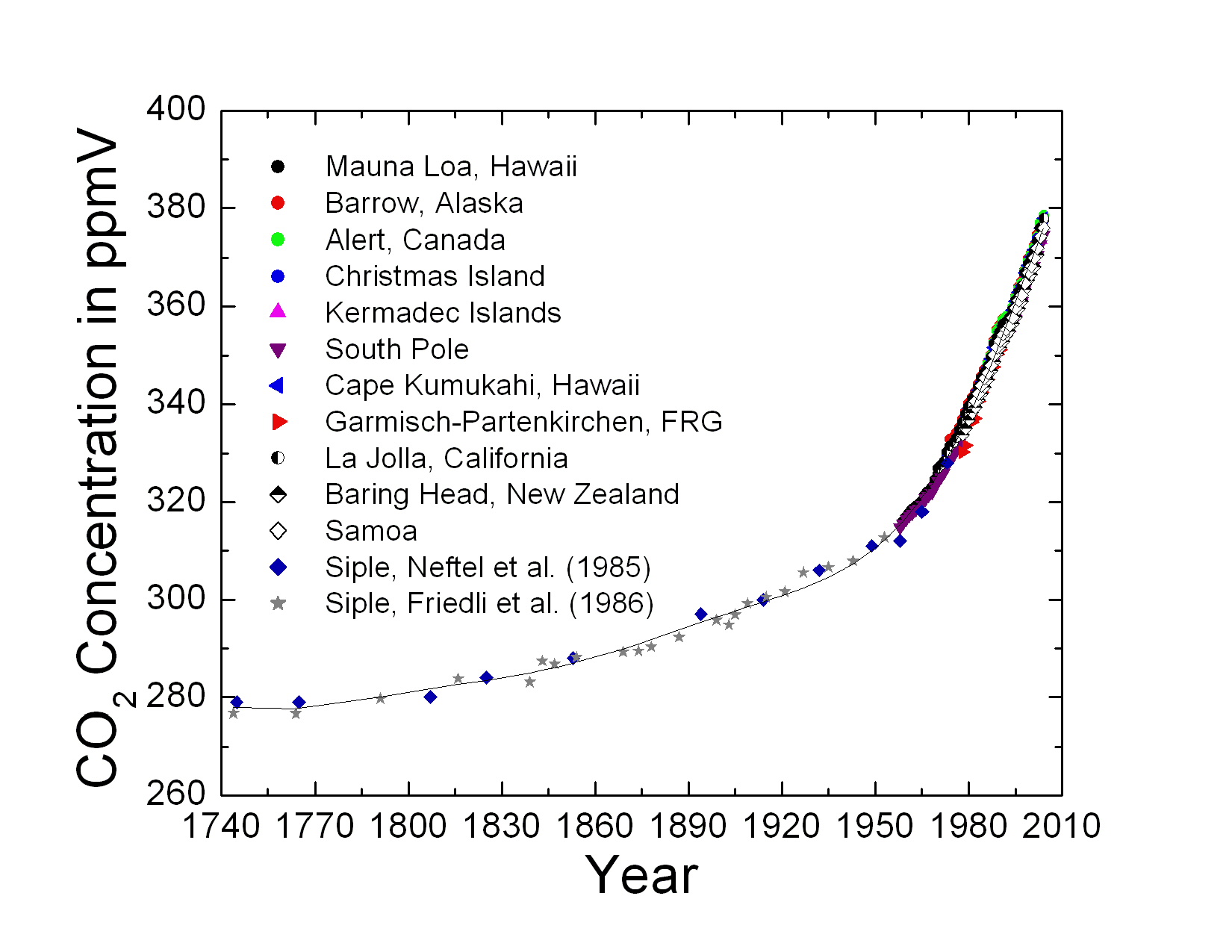
Figure 4: Atmospheric $CO_{2}$ concentration inferred from Siple station (West Antarctica) ice cores analyzed by Neftel et al. [49] and Friedli et al. [19] and extended to that directly observed at various locations during the period 1958-2004 (courtesy of C.D. Keeling, T.P. Whorf, and the Carbon Dioxide Research Group of the Scripps Institution of Oceanography (SIO). The fit is based of a polynomial of $8^{th}$ order.

8 The global budget of carbon dioxide

Dividing Eq. (7) by the volume and rearranging the resulting equation yield for a turbulent system

$$\Bigl{\langle}\frac{\partial{\overline{\rho_{i}}}}{\partial{t}}\Bigr{\rangle}_{V}=-\;\frac{1}{V(t)}\;\int_{A(V(t))}\bigl{(}\overline{\rho_{i}}\;\overline{\textbf{v}}+\overline{\rho_{i}^{\prime}\;\textbf{v}^{\prime}}+\overline{\textbf{J}_{i}}\bigr{)}\cdot d\textbf{A}+\bigl{\langle}\overline{\sigma_{i}}\bigr{\rangle}_{V}\;,$$ (56)

where the volume average of an arbitrary quantity $\psi$ is generally defined by

$$\bigl{\langle}\psi\bigr{\rangle}_{V}=\frac{1}{V}\int_{V}\psi\;V\;.$$ (57)

Hitherto, the volume $V(t)$ has been considered as arbitrary. Suppose the earth can be considered as a sphere with the radius $r_{E}\cong 6,371$ km and the atmospheric layer under study that directly covers the earth as a spherical shell of a thickness of $\Delta r$, the volume of the atmospheric layer, $V_{A}$, now considered as independent of time is then given by

$$V_{A}=\frac{4}{3}\;\pi\;r_{E}^{3}\;\Bigl{\{}\Bigl{(}1+\frac{\Delta r}{r_{E}}\Bigr{)}^{3}-1\Bigr{\}}\;.$$ (58)

Since $\Delta r/r_{E}\ll 1$, the term $(1+\Delta r/r_{E})^{3}$ can be approximated by $1+3\;\Delta r/r_{E}$. Thus, we obtain

$$V_{A}=4\;\pi\;r_{E}^{2}\;\Delta r\;.$$ (59)

The surface of this spherical shell is given by $A_{A}=A_{T}+A_{E}=4\;\pi\;r_{E}^{2}\;\{(1+\Delta r/r_{E})^{2}+2\}$, where $A_{T}$ and $A_{E}$ are the outer surface and the inner surface of this shell, respectively. The latter is congruent with the earth’s surface. The surface integral in Eq. (56) may, therefore, be expressed by

$$\int_{A_{A}}\bigl{(}\overline{\rho_{i}}\;\overline{\textbf{v}}+\overline{\rho_{i}^{\prime}\;\textbf{v}^{\prime}}+\overline{\textbf{J}_{i}}\bigr{)}\cdot d\textbf{A}=\int_{A_{T}}\bigl{(}\overline{\rho_{i}}\;\overline{\textbf{v}}+\overline{\rho_{i}^{\prime}\;\textbf{v}^{\prime}}+\overline{\textbf{J}_{i}}\bigr{)}\cdot d\textbf{A}$$ (60)

$$+ \int_{A_{E}}\bigl{(}\overline{\rho_{i}}\;\overline{\textbf{v}}+\overline{\rho_{i}^{\prime}\;\textbf{v}^{\prime}}+\overline{\textbf{J}_{i}}\bigr{)}\cdot d\textbf{A}\;.$$

The first integral on the right-hand side of this equation describes the exchange of matter between the atmospheric layer under study and the atmospheric region aloft across the common border, and the second integral the exchange of matter between the atmospheric layer under study and the earth caused by the total (anthropogenic plus natural) emission (counted positive) and the uptake (counted negative) by the terrestrial biosphere (plants and soils) and the oceans. If we choose $\Delta r$ in such a sense that exchange across the outer surface of this spherical shell is equal to zero (or in comparison with that at the earth’s surface, at least, negligible) because of the vertical profile of the $CO_{2}$ concentration becomes (nearly) independent of height (see, e.g., Figure 1 in [63]), we will obtain

$$\int_{A_{A}}\bigl{(}\overline{\rho_{i}}\;\overline{\textbf{v}}+\overline{\rho_{i}^{\prime}\;\textbf{v}^{\prime}}+\overline{\textbf{J}_{i}}\bigr{)}\cdot d\textbf{A}=\int_{A_{E}}\bigl{(}\overline{\rho_{i}}\;\overline{\textbf{v}}+\overline{\rho_{i}^{\prime}\;\textbf{v}^{\prime}}+\overline{\textbf{J}_{i}}\bigr{)}\cdot d\textbf{A}\;.$$ (61)

Since the unit vector normal to the inner surface of the spherical shell shows in the direction of the earth’s center, we have only to consider the radial components of these fluxes characterized by the subscript $r$, i.e.,

$$\int_{A_{E}}\bigl{(}\overline{\rho_{i}}\;\overline{\textbf{v}}+\overline{\rho_{i}^{\prime}\;\textbf{v}^{\prime}}+\overline{\textbf{J}_{i}}\,\bigr{)}\cdot d\textbf{A}=-\;\int_{A_{E}}\bigl{(}\overline{\rho_{i}}\;\overline{v_{r}}+\overline{\rho_{i}^{\prime}\;v_{r}^{\prime}}+\overline{J_{r,i}}\,\bigr{)}\Bigr{|}_{EM}dA$$ (62)

$$+ \int_{A_{E}}\bigl{(}\overline{\rho_{i}}\;\overline{v_{r}}+\overline{\rho_{i}^{\prime}\;v_{r}^{\prime}}+\overline{J_{r,i}}\,\bigr{)}\Bigr{|}_{U}dA\;.$$

The first integral on the right-hand side of this equation represents the total emission (subscript $EM$) and the second one the uptake (subscript $U$). The signs of these terms are determined by the scalar product between the unit vectors of the fluxes and the unit vector normal to the inner surface of the spherical shell.
Combining Eqs. (56) and (60) to (62) yields

$$\Bigl{\langle}\frac{\partial{\overline{\rho_{i}}}}{\partial{t}}\Bigr{\rangle}_{V_{A}} = \frac{1}{V_{A}}\;\Bigl{\{}\int_{A_{E}}\bigl{(}\overline{\rho_{i}}\;\overline{v_{r}}+\overline{\rho_{i}^{\prime}\;v_{r}^{\prime}}+\overline{J_{r,i}}\,\bigr{)}\Bigr{|}_{EM}dA$$ (63)

$$- \int_{A_{E}}\bigl{(}\overline{\rho_{i}}\;\overline{v_{r}}+\overline{\rho_{i}^{\prime}\;v_{r}^{\prime}}+\overline{J_{r,i}}\,\bigr{)}\Bigr{|}_{U}dA\Bigr{\}}+\bigl{\langle}\overline{\sigma_{i}}\bigr{\rangle}_{V_{A}}\;.$$

Since $CO_{2}$ is a long-lived trace gas, the effect caused by chemical reactions can be ignored. Thus, Eq. (63) can be approximated by

$$\Bigl{\langle}\frac{\partial{\overline{\rho_{i}}}}{\partial{t}}\Bigr{\rangle}_{V_{A}} = \frac{1}{V_{A}}\;\Bigl{\{}\int_{A_{E}}\bigl{(}\overline{\rho_{i}}\;\overline{v_{r}}+\overline{\rho_{i}^{\prime}\;v_{r}^{\prime}}+\overline{J_{r,i}}\,\bigr{)}\Bigr{|}_{EM}dA$$

$$- \int_{A_{E}}\bigl{(}\overline{\rho_{i}}\;\overline{v_{r}}+\overline{\rho_{i}^{\prime}\;v_{r}^{\prime}}+\overline{J_{r,i}}\,\bigr{)}\Bigr{|}_{U}dA\Bigr{\}}\;.$$

Expanding the right-hand side of this equation with $A_{E}$ yields finally

$$\Bigl{\langle}\frac{\partial{\overline{\rho_{i}}}}{\partial{t}}\Bigr{\rangle}_{V_{A}} = \frac{1}{\Delta r}\;\Bigl{\{}\Bigl{\langle}\bigl{(}\overline{\rho_{i}}\;\overline{v_{r}}+\overline{\rho_{i}^{\prime}\;v_{r}^{\prime}}+\overline{J_{r,i}}\,\bigr{)}\Bigr{|}_{EM}\Bigr{\rangle}_{A_{E}}$$ (65)

$$- \Bigl{\langle}\bigl{(}\overline{\rho_{i}}\;\overline{v_{r}}+\overline{\rho_{i}^{\prime}\;v_{r}^{\prime}}+\overline{J_{r,i}}\,\bigr{)}\Bigr{|}_{U}\Bigr{\rangle}_{A_{E}}\Bigr{\}}\;,$$

where

$$\bigl{\langle}\psi\bigr{\rangle}_{A_{E}}=\frac{1}{A_{E}}\int_{A_{E}}\psi\;dA\;.$$ (66)

represents the global average of an arbitrary quantity $\psi$. Equation (65) deduced by using the exact integral formulations substantiates that (a) total emission and the uptake of $CO_{2}$ have to be considered as lower boundary conditions and (b) the partial density of $CO_{2}$ averaged over the volume of the atmospheric layer under study will rise as long as the globally averaged total emission is higher than the globally averaged uptake.

9 Final remarks and conclusions

In 1999 Sarmiento and Gruber [60] pointed out that ”the land sink for carbon is the subject of considerable controversy at present, concerning not only its magnitude but also its cause”. It seems that any use of an alternative mass balance equation in micrometeorology may contribute to considerably more confusion because this alternative expression is clearly incorrect.
The use of an alternative mass balance equation can harmfully affect not only the whole atmospheric budget of $CO_{2}$, but also that of other greenhouse gases like water vapor (the most important greenhouse gas), nitrous oxide ($N_{2}O$), methane ($CH_{4}$), and ozone ($O_{3}$).
If Eqs. (19) and (27) are correct, the biological source/sink, for instance, would explicitly cause a temporal change in the partial density. However, the reality is different. Figure 4 illustrates that the atmospheric $CO_{2}$ concentration has been rising since the beginning of the 18th century. If these results are correct as stated in various reports of the Intergovernmental Panel on Climate Change (IPCC), we can infer from Eq. (65) that the total emission of $CO_{2}$ has always been higher than the $CO_{2}$ uptake during the period covered by these results. Thus, lowering, for instance, the anthropogenic emissions of $CO_{2}$ to those of the year 1990 would not reduce the $CO_{2}$ concentration in the atmosphere (see Special Report on Emissions Scenarios (SRES) of the Working Group III of the Intergovernmental Panel on Climate Change (IPCC) and the IPCC IS92, [25, 27]). However, if the $CO_{2}$ uptake would rise due to a higher atmospheric $CO_{2}$ concentration, a stabilization of this concentration at a level of nearly 550 ppmV, i.e., higher than that of 1990, might be possible [25, 27].
A decrease of the atmospheric $CO_{2}$ concentration can only be achieved when the $CO_{2}$ uptake by the terrestrial biosphere and the ocean is higher than the total emission $CO_{2}$. As indicated by Beck’s[4] inventory for the past 180 years that is based on more than 90,000 observations using chemical methods, there were $CO_{2}$ concentrations appreciably higher than the current value of about 385 $ppmV$. Only when Beck’s data are reliable, we may conclude that during various periods of the past the uptake was stronger than the total emission.

References

References

- [1] Allan, D.W. 1966. Statistics of atomic frequency standards. Proceedings IEEE 54, 221-230.
- [2] Aubinet, M., Heinesch, B., and Yernaux, M. 2003. Horizontal and vertical advection in a sloping forest. Boundary-Layer Meteorol. 108, 397-417.
- [3] Barenblatt, G.I., 1996: Similarity, Self-Similarity, and Intermediate Asymptotics. Cambridge University Press, Cambridge, U.K., 386 pp.
- [4] Beck, E.G. 2007. 180 years of atmospheric gas analysis by chemical method. Energy and Environment 18, 259-282.
- [5] Bracewell, R. 1999. The Fourier Transform and its Applications. McGraw-Hill, New York, 640 pp.
- [6] Brunet, Y. and Collineau, S. 1994. Wavelet analysis and nocturnal turbulence above a maize-crop. In: Foufoula-Georgiou, E. and Kumar, P. (eds.), Wavelets in Geophysics. Academic Press, San Diego, CA, pp. 129-150.
- [7] Buckingham, E., 1914. On physically similar systems; illustrations of the use of dimensional equations. Physical Review 4, 345-376.
- [8] Busch, N.E. 1973. On the mechanics of atmospheric turbulence. In: haugen, D.A. (ed.), Workshop on Micrometeorology. American Meteorological Society, Boston, Mass., pp. 1-65.
- [9] Businger, J.A. 1986. Evaluation of the accuracy with which dry deposition can be measured with current micrometeorological techniques. J. Appl. Meteor. 25, 1100-1124.
- [10] de Groot, S.R. and Mazur, P. 1969. Non-Equilibrium Thermodynamics. North-Holland Publishing Comp., Amsterdam/London, 514 pp.
- [11] Dirac, P.A.M. 1958. The Principles of Quantum Mechanics. Oxford University Press, Oxford, UK, 314 pp.
- [12] Dutton, J.A. 1995. Dynamics of Atmospheric Motion. Dover, New York, 617 pp.
- [13] Falkovich, G. and Sreenivasan, K.R. 2006. Lessons from hydrodynamic turbulence. Physics Today 59 (4), 43-49.
- [14] Feigenwinter, C., Bernhofer, C., and Vogt, R. 2004. The influence of advection on the short-term -budget in and above a forest canopy. Boundary-Layer Meteorol. 113, 201-224.
- [15] Finnigan, J.J., Clement, R., Malhi, Y., Leuning, R., and Cleugh, H.A. 2003. A re-evaluation of long-term flux measurement techniques, Part I: Averaging and coordinate rotation. Boundary-Layer Meteorol. 107, 1-48.
- [16] Finnigan, J.J. 2004a. A re-evaluation of long-term flux measurement techniques, Part II: Coordinate systems. Boundary-Layer Meteorol. 113, 1-41.
- [17] Finnigan, J.J. 2004b. Advection and modeling. In: Lee, X., Massman, W., and Law, B. (eds.), Handbook of Micrometeorology: A Guide for Surface Flux Measurement and Analysis. Kluwer Academic Publishers, Boston, pp. 209-244.
- [18] Flandrin, P. 1992. Wavelet analysis and synthesis of fractional Brownian motion. IEEE Tans. Info. Theo. 38, 910-917.
- [19] Friedli, H., L tscher, H., Oeschger, H., Siegenthaler, U., and Stauffer, B. 1986. Ice core record of the ratio of atmospheric in the past two centuries. Nature 324, 237-238.
- [20] Garratt, J.R. 1992. The Atmospheric Boundary Layer. Cambridge University Press, 316 pp.
- [21] Hagelberg, C.R. and Gamage, N.K.K. 1994. Applications of structure preserving wavelet decompositions to intermittent turbulence: A case study. In: Foufoula-Georgiou, E. and Kumar, P. (eds.), Wavelets in Geophysics. Academic Press, San Diego, CA, pp. 45-80.
- [22] Herbert, F. 1975. Irreversible Prozesse der Atmosph re - 3. Teil (Ph nomenologische Theorie mikroturbulenter Systeme). Beitr. Phys. Atmosph. 48, 1-29 (in German).
- [23] Herbert, F. 1980. Prigogine’s diffusion theorem and its application to atmospheric transfer processes, Part 1: The governing theoretical concept. Beitr. Phys. Atmosph. 53, 181-203.
- [24] Herbert, F. 1983. Prigogine’s diffusion theorem and its application to atmospheric transfer processes, Part 2: Invariance properties and Fick type diffusion laws. Beitr. Phys. Atmosph. 56, 480-494.
- [25] Houghton, J.T., Ding, Y., Griggs, D.J., Noguer, M., van der Linden, P.J., Dai, X., Maskell, K., and Johnson, C.A. (eds.). 2001. Climate Change 2001: The Scientific Basis. Contribution of Working Group I to the Third Assessment Report of the Intergovernmental Panel on Climate Change. Intergovernmental Panel on Climate Change. Cambridge University Press, Cambridge, UK, 881 pp.
- [26] Howell, J.F. and Mahrt, L. 1994. An adaptive decomposition: Application to turbulence. In Foufoula-Georgiou, E. and Kumar, P. (eds.), Wavelets in Geophysics. Academic Press, San Diego, CA, pp. 107-128.
- [27] Kattsov, V.M. and K ll n, E. (lead authors). 2005. Arctic Climate Impact Assessment 2004 Report (Chapter 4), Future climate change: Modeling and scenarios for the Arctic. Cambridge University Press, Cambridge, UK, 52 pp.
- [28] Katul, G.G., Albertson, J.D., Chu, C.R., and Parlange, M.B. 1994. Intermittency in atmospheric surface layer turbulence: The orthogonal wavelet representation. In: Foufoula-Georgiou, E. and Kumar, P. (eds.), Wavelets in Geophysics. Academic Press, San Diego, CA, pp. 81-106.
- [29] Kramm, G., 1989. A numerical method for determining the dry deposition of atmospheric trace gases. Boundary-Layer Meteorol. 48, 157-176.
- [30] Kramm, G., Dlugi, R., and Lenschow, D.H. 1995. A re-evaluation of the Webb-correction using density-weighted averages. J. Hydrol. 166, 283-292.
- [31] Kramm, G., Beier, N., Dlugi, R., and M ller, H. 1999. Evaluation of conditional sampling methods. Contr. Atmos. Phys. 72, 161-172.
- [32] Kramm, G. and Meixner, F.X., 2000. On the dispersion of trace species in the atmospheric boundary layer: A re-formulation of the governing equations for the turbulent flow of the compressible atmosphere. Tellus 52A, 500-522.
- [33] Kramm, G. 2004. Sodar data and scintillometer data obtained from the UPOS project ”Optical Turbulence” and applied to study the turbulence structure in the atmospheric surface layer. Report of the Geophysical Institute, 89 pp.
- [34] Kramm, G. and Dlugi, R. 2006. On the correction of eddy fluxes of water vapour and trace gases. J. Calcutta Math. Soc. 2, 29-54.
- [35] Kramm, G. and Herbert, F. 2008. Similarity hypotheses for the atmospheric surface layer expressed by dimensional invariants analysis - a review (submitted).
- [36] Kumar, P. and Foufoula-Georgiou, E. 1997. Wavelet analysis for geophysical applications. Rev. Geophys. 35, 385-412.
- [37] Landau, L.D. and Lifshitz, E.M. 1959. Course of Theoretical Physics - Vol. 6) Fluid Mechanics. Pergamon Press, Oxford/New York/Toronto/Sydney/Paris/Frankfurt, 536 pp.
- [38] Landau, L.D. and Lifshitz, E.M. 1977. Course of Theoretical Physics - Vol. 3) Quantum Mechanics. Pergamon Press, Oxford/New York/Toronto/Sydney/Paris/Frankfurt, 673 pp.
- [39] Lee, X., Finnigan, J.J., and Paw U, K.T. 2004a. Coordinate systems and flux bias error. In: Lee, X., Massman, W., and Law, B. (eds.), Handbook of Micrometeorology: A Guide for Surface Flux Measurement and Analysis. Kluwer Academic Publishers, Boston, pp. 33-66.
- [40] Lee, X., Massman, W., and Law, B. (eds.), 2004b. Handbook of Micrometeorology: A Guide for Surface Flux Measurement and Analysis. Kluwer Academic Publishers, Boston, 250 pp.
- [41] Liepmann, H.V. 1952. Aspects of the turbulence problem. Z. angew. Math. Phys. 3, 1th part, 321-342, 2nd part, 407-426.
- [42] Liu, H. 2005. An alternative approach for flux correction caused by heat and water vapour transfer. Boundary-Layer Meteorol. 115, 151-168.
- [43] Lumley, J.L. and Panofsky, H.A. 1964. Atmospheric Turbulence. Interscience Publishers, New York/London/Sydney, 239 pp.
- [44] Massman, W.J. and Tuovinen, J.P. 2006. An analysis and implications of alternative methods of deriving the density(WPL) terms for eddy covariance flux measurements. Boundary-Layer Meteorol. 121, 221-227.
- [45] McRae, G.J. and Russell, A.G. 1984. Dry deposition of nitrogen-containing species. In: Hicks, B.B. (ed.), Deposition both Wet and Dry. Acid precipitation series - Vol. 4, Butterworth Publishers, Boston/London, pp. 153-193.
- [46] Messiah, A. 1961. Quantum Mechanics - Volume I. North-Holland Publishing Company, Amsterdam, The Netherlands, and J. Wiley & Sons, New York/London, 504 pp.
- [47] Moncrieff, J., Clement, R., Finnigan, J., and Meyers, T. 2004. Averaging, detrending, and filtering of eddy covariance time series. In: Lee, X., Massman, W., and Law, B. (eds.), Handbook of Micrometeorology: A Guide for Surface Flux Measurement and Analysis. Kluwer Academic Publishers, Boston, pp. 7-31.
- [48] Monin, A.S. and Obukhov, A.M. 1954. Osnovnye zakonomernosti turbulentnogo peremesivanija v prizemnom sloe atmosfery. Trudy geofiz inst AN SSSR 24 (151), 163-187 (in Russian).
- [49] Neftel, A., Moor, E., Oeschger, H., and Stauffer, B. 1985. Evidence from polar ice cores for the increase in atmospheric in the past two centuries. Nature 315, 45-47.
- [50] Obukhov, A.M. 1946. Turbulentnost’ v temperaturno-neodnorodnoj atmosphere. Trudy Inst. Teoret. Geofiz. AN. SSSR. 1 (in Russian; English translation in Boundary-Layer Meteorol. 2, 7-29, 1971).
- [51] Panofsky, H.A. 1963. Determination of stress from wind and temperature measurements. Quart. J. R. Met. Soc. 89, 85-94.
- [52] Panofsky, H.A. and Dutton, J.A. 1984. Atmospheric Turbulence. New York/Chichester/ Brisbane/Toronto/Singapore: John Wiley & Sons, 397 pp.
- [53] Paulson, C.A. 1970. The mathematical representation of wind speed and temperature profiles in the unstable atmospheric surface layer. J. Appl. Meteor. 9, 857-861.
- [54] Percival, D.B. and Guttorp, P. 1994. Long-memory processes, the Allan variance and wavelets. In: Foufoula-Georgiou, E. and Kumar, P. (eds.), Wavelets in Geophysics. Academic Press, San Diego, CA, pp. 325-344.
- [55] Pichler, H. 1984. Dynamic der Atmosph re. Bibliographisches Institut, Z rich, 456 pp. (in German).
- [56] Pielke, R.A., Sr., 2002. Mesoscale Meteorological Modeling. 2nd Edition, Academic Press, San Diego, CA., 672 pp.
- [57] Prigogine, I. 1947. tude thermodynamique des ph nom nes irr versibles. Thesis, Dunod, Paris, and Desoer, Li ge.
- [58] Raupach, M.R. 2001. Inferring biochemical sources and sinks from atmospheric concentrations: General consideration and applications in vegetation canopies. In: Schulze E.D. et al (eds.), Global Biochemical Cycles in the Climate System. Academic Press, San Diego/San Francisco/New York/Boston/London/Sydney/ Tokyo, pp. 41-59.
- [59] Riley, K.F., Hobson, M.P., and Bence, S.J. 1998. Mathematical Methods for Physics and Engineering. Cambridge University Press, Cambridge, UK, 1008 pp.
- [60] Sarmiento, J.L. and Gruber, N. 2002. Sinks for anthropogenic carbon. Physics Today 55 (8), 30-36.
- [61] Seinfeld, J.H. and Pandis, S.N. 1998. Atmospheric Chemistry and Physics. John Wiley & Sons, New York/Chichester/Weinheim/Brisbane/ Singapore/Toronto, 1326 pp.
- [62] Sogachev, A. and Lloyd, J. 2004. Using a one-and-a-half order closure model of the atmospheric boundary layer for surface flux footprint estimation. Boundary-Layer Meteorol. 112, 467-502.
- [63] Stephens, B.B., Gurney, K.R., Tans, P.P., Sweeney, C., Peters, W., Bruhwiler, L., Ciais, P., Ramonet, M., Bousquet, P., Nakazawa, T., Aoki, S., Machida, T., Inoue, G., Vinnichenko, N., Lloyd, J., Jordan, A., Heimann, M., Shibistova, O., Langenfelds, R.L., Steele, L.P., Francey, R.J., and Denning, A.S. 2007. Weak northern and strong tropical land carbon uptake from vertical profiles of atmospheric . Science 316, 1732-175.
- [64] Stull, R.B. 1988. An Introduction to Boundary Layer Meteorology. Kluwer Academic Publishers, Dordrecht, 666 pp.
- [65] Sun, J. 2007. Tilt corrections over complex terrain and their implication for transport. Boundary-Layer Meteorol. 124, 143-159.
- [66] Sun, J., Burns, S.P., Delany, A.C., Oncley, S.P., Turnipseed, A.A., Stephens, B.B., Lenschow, D.H., LeMone, M.A. 2007. transport over complex terrain. Agric. Forest. Meteorol. 145, 1-21.
- [67] Tennekes, H. and Lumley, J.L. 1972. A First Course in Turbulence. MIT Press, Cambridge, MA, 300 pp.
- [68] Trevi o, G. and Andreas, E.L. 2006. Averaging operators in turbulence. Physics Today 59 (11), 16-17.
- [69] van Mieghem, J. 1973. Atmospheric Energetics. Clarendon Press, Oxford, 306 pp.
- [70] Werle, P., M cke, R., and Slemr, F. 1993. The limits of signal averaging in atmospheric trace-gas monitoring by tunable diode-laser absorption spectroscopy (TDLAS). Appl. Phys. B57, 131-139.
- [71] Werle, P., Kormann, R., M cke, R., Foken, T., Kramm, G., and M ller, H. 1996. Analysis of time series data: A time domain stability criterion for stationarity tests. In: Borrell, P. et al (eds.), Transport and Transformation of Pollutants in the Troposphere, Vol. 2, Proceedings of the EUROTRAC Symposium ’96. Computational Mechanics Publications, Southampton, Boston, pp. 703-707.
- [72] Zilitinkevich, S.S. 1966. Effects of humidity stratification on hydrostatic stability. Izv. Atmos. Ocean. Phys. 2, 655-658.