Charmed Meson Dalitz Plot Analyses at BABAR

Abstract

We report recent results of the Dalitz plot analyses of $D$ and $D_{S}$ decays performed by the BABAR collaboration, and point out some of the important applications of these results.

I Introduction

The amplitudes describing $D$ and $D_{s}$ meson weak decays into final states with three pseudo-scalers are dominated by intermediate resonances that lead to highly nonuniform intensity distributions in the available phase space. The results of the Dalitz plot analysis of these decays are playing increasingly important role in flavor physics, particularly in the extraction of the $C\!P$-violating phase $\gamma=\arg{\left(-V_{ud}V_{ub}^{\ast}/V_{cd}V_{cb}^{\ast}\right)}$ of the quark mixing (i.e., CKM) matrix by exploiting interference structure in the $D$ Dalitz plot from the decay $B^{\pm}\rightarrow DK^{\pm}$ myGamma and in the measurement of $D^{0}$–$\kern 1.99997pt\overline{\kern-1.99997ptD}{}^{0}$ mixing parameters.

II Detector

We perform these analyses using $e^{+}e^{-}$ collision data collected at and around 10.58 GeV center-of-mass (CM) energy with the BABAR detector detector at the PEP-II storage ring. Tracking of charged particles is provided by silicon detector and a drift chamber operating in a 1.5-T magnetic field. Particle types are identified using specific ionization energy loss measurements in the two tracking devices and Cherenkov photons detected in a ring-imaging detector. The energy of photons and electrons is measured with an electromagnetic calorimeter. In case of neutral $D$-meson decays, we distinguish $D^{0}$ from $\kern 1.99997pt\overline{\kern-1.99997ptD}{}^{0}$ by reconstructing the decays $D^{*+}\rightarrow D^{0}\pi^{+}$ and $D^{*-}\rightarrow\kern 1.99997pt\overline{\kern-1.99997ptD}{}^{0}\pi^{-}$. For each decay mode, we estimate the signal efficiency as a function of position in the Dalitz plot using simulated signal events generated uniformly in the available phase space, subjected to the same reconstruction procedure applied to the data, and corrected for differences in particle-identification rates in data and simulation.

III Dalitz plot parametrization

The complex quantum mechanical amplitude $\cal{A}$ that describes decays to three particles $A$, $B$ and $C$ in the final state can be characterized as a coherent sum of all relevant quasi-two-body $D/D_{s}\rightarrow(r\rightarrow AB)C$ isobar model resonances, ${\cal{A}}=\sum_{r}a_{r}e^{i\phi_{r}}A_{r}(s)$. Here $s=m_{AB}^{2}$, and $A_{r}$ is the resonance amplitude. We obtain the coefficients $a_{r}$ and $\phi_{r}$ from a likelihood fit. The probability density function for signal events is $\left|\cal{A}\right|^{2}$.

Unless stated otherwise, for S-, P-, and D-wave (spin = 0, 1, and 2, respectively) resonant states we use the Breit-Wigner amplitude:

$$A_{BW}(s) = {{\cal{M}}_{L}(s,p)}\hskip 2.0pt{1\over{M_{0}^{2}-s-iM_{0}\Gamma(s)}},$$ (1)

$$\Gamma(s) = \Gamma_{0}\Big{(}{M_{0}\over\sqrt{s}}\Big{)}\Big{(}{p\over{p_{0}}}\Big{)}^{2L+1}{\Big{[}{{\cal{F}}_{L}(p)\over{\cal{F}}_{L}(p_{0})}\Big{]}^{2}},$$ (2)

where $M_{0}$ ($\Gamma_{0}$) is the resonance mass (width) pdg , $L$ is the angular momentum quantum number, $p$ is the momentum of either daughter in the resonance rest frame, and $p_{0}$ is the value of $p$ when s = $M_{0}^{2}$. The function ${\cal{F}}_{L}$ is the Blatt-Weisskopf barrier factor bw : ${{{\cal{F}}_{0}}}$ = 1, ${{{\cal{F}}_{1}}}$ = $1/\sqrt{1+{Rp}^{2}}$, and ${{{\cal{F}}_{2}}}$ = $1/\sqrt{9+3{Rp}^{2}+{Rp}^{4}}$, where we take the meson radial parameter $R$ to be 1.5 GeV^-1. The quantity ${{\cal{M}}_{L}}$ is the spin part of the amplitude: ${{\cal{M}}_{0}}$ = constant, ${{\cal{M}}_{1}}\propto-2\vec{p_{A}}.\vec{p_{C}}$, and ${{\cal{M}}_{2}}$ $\propto{4\over 3}\left[3{(\vec{p_{A}}.\vec{p_{C}})}^{2}-{|\vec{p_{A}}|}^{2}.{|\vec{p_{C}}|}^{2}\right]$, where $\vec{p_{i}}$ is the 3-momentum of particle $i$ in the resonance rest frame. The fit fraction for a resonant process $r$ is defined as $f_{r}\equiv\int\left|a_{r}A_{r}\right|^{2}d\tau/\int\left|{\cal{A}}\right|^{2}d\tau$, where $d\tau$ is a phase-space element. Due to interference among the contributing amplitudes, the $f_{r}$ do not sum to one in general. In all cases, we model small incoherent background empirically from data.

IV Angular moments

For $D$ and $D_{s}$ decays to three spinless particles, the Dalitz plot uniquely represents the kinematics of the final state. The angular distributions provide further information on the detailed event-density variations in various regions of the phase space in a different form. We define the helicity angle $\theta_{H}$ for decays $D^{0}\rightarrow(r\rightarrow AB)C$ as the angle between the momentum of $A$ in the $AB$ rest frame and the momentum of $AB$ in $D^{0}$ rest frame. The moments of the cosine of the helicity angle, $Y_{l}^{0}(\cos\theta_{H})$, are defined as the efficiency-corrected invariant mass distributions of events when weighted by spherical harmonic functions

$$Y_{l}^{0}(\theta_{H})=\sqrt{1\over{2\pi}}~{}P_{l}(m),$$ (3)

where $m$ is the invariant mass of the $AB$ system and the $P_{l}$ are Legendre polynomials of order $l$:

$$\int\limits_{-1}^{1}{P_{l}(x)~{}P_{n}(x)~{}dx}=\delta_{ln}.$$ (4)

These angular moments have an obvious physical significance. Since spherical harmonic functions are the eigen-functions of the angular momentum, the Dalitz plot of a three-body decay can be represented by the sum of an infinite number of spherical harmonic moments in any two-body channel. In a region of the Dalitz plot where S- and P-waves in a single channel dominate, their amplitudes are given by the following Legendre polynomial moments,

$$P_{0} = \frac{{\left|S\right|}^{2}+{\left|P\right|}^{2}}{\sqrt{2}},$$

$$P_{1} = {\sqrt{2}}{\left|S\right|}{\left|P\right|}~{}\cos\theta_{SP},$$

$$P_{2} = {\sqrt{2\over 5}}~{}{\left|P\right|^{2}},$$ (5)

where $\left|S\right|$ and $\left|P\right|$ are, respectively, the magnitudes of the S- and P-wave amplitudes, and $\theta_{SP}=\theta_{\textit{S}}-\theta_{P}$ is the relative phase between them. It is worth noting that this partial-wave analysis is valid, in the absence of higher spin states, only if no interference occurs from the crossing channels.

V Dalitz plot analysis of $D^{0}\rightarrow K^{-}K^{+}\pi^{0}$

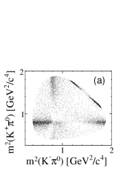
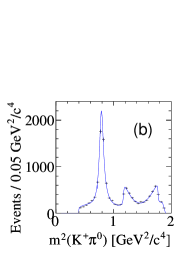
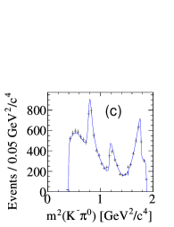
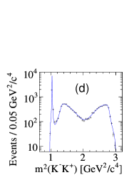
Figure 1: Dalitz plot for $D^{0}\rightarrow K^{-}K^{+}\pi^{0}$ mykkpi0 data (a), and the corresponding squared invariant mass projections (b–d). In plots (b–d), the dots with error bars are data points and the solid lines correspond to the best isobar fit models.

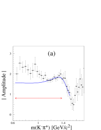
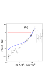
Figure 2: LASS (solid line) and E-791 (dots with error bars) $K\pi$ S-wave amplitude (a) and phase (b). The double headed arrow indicates the mass range available in $D^{0}\rightarrow K^{-}K^{+}\pi^{0}$.

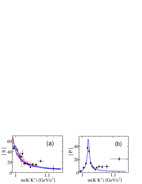
Figure 3: The phase-space-corrected $K^{-}K^{+}$ S- and P-wave amplitudes, $\left|S\right|$ and $\left|P\right|$, respectively. (a) Lineshapes for (solid line, blue) $f_{0}(980)$, and (broken line, blue) $a_{0}(980)$. (b) Lineshape for $\phi(1020)$ (solid line, blue). In each plot, solid circles with error bars correspond to values obtained from the model-independent analysis. In (a), the open triangles (red) correspond to values obtained from the decay $D^{0}\rightarrow K^{-}K^{+}\bar{K^{0}}$.

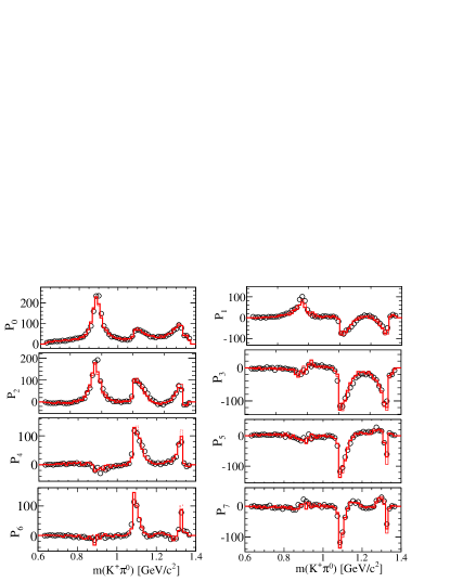
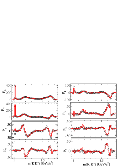
Figure 4: Legendre polynomials moments for the $K^{+}\pi^{0}$ (columns I, II) and $K^{-}K^{+}$ (columns III, IV) channels of $D^{0}\rightarrow K^{-}K^{+}\pi^{0}$. The circles with error bars are data points and the curves (red) are derived from the fit functions.

The $K^{\pm}\pi^{0}$ systems from the decay $D^{0}\rightarrow K^{-}K^{+}\pi^{0}$ note1 can provide information on the $K\pi$ S-wave amplitude in the mass range 0.6–1.4 ${\mathrm{\,Ge\kern-1.00006ptV\!/}c^{2}}$, and hence on the possible existence of the $\kappa(800)$, reported to date only in the neutral state ($\kappa^{0}\rightarrow K^{-}\pi^{+}$) kappa . If the $\kappa$ has isospin $1/2$, it should be observable also in the charged states. Results of the present analysis can be an input for extracting the CKM phase $\gamma$ by exploiting interference in the Dalitz plot from the decay $B^{\pm}\rightarrow D^{0}_{K^{-}K^{+}\pi^{0}}K^{\pm}$ myGamma .
We perform the analysis on 385 fb^-1 data using the same event-selection criteria as in our measurement of the branching ratio of the decay $D^{0}\rightarrow K^{-}K^{+}\pi^{0}$ mybr . To minimize uncertainty from background shape, we choose a high purity ($\sim$$98\%$) sample using $1855<m_{D^{0}}<1875$ ${\mathrm{\,Me\kern-1.00006ptV\!/}c^{2}}$, and find $11278\pm 110$ signal events. The Dalitz plot for these events is shown in Fig. 1(a).

For $D^{0}$ decays to $K^{\pm}\pi^{0}$ S-wave states, we consider three amplitude models: LASS amplitude for $K^{-}\pi^{+}\rightarrow K^{-}\pi^{+}$ elastic scattering LASS ; mykkpi0 , the E-791 results for the $K^{-}\pi^{+}$ S-wave amplitude from a partial-wave analysis of the decay $D^{+}\rightarrow K^{-}\pi^{+}\pi^{+}$ brian , and a coherent sum of a uniform nonresonant term plus Breit-Wigner terms for $\kappa(800)$ and $K^{*}_{0}(1430)$ resonances.

In Fig. 2 we compare the $K\pi$ S-wave amplitude from the E-791 analysis brian to the LASS amplitude. The LASS $K\pi$ S-wave amplitude gives the best agreement with data and we use it in our nominal fits ($\chi^{2}$ probability 62%). The $K\pi$ S-wave modeled by the combination of $\kappa(800)$ (with parameters taken from Ref. kappa ), a nonresonant term and $K^{*}_{0}(1430)$ has a smaller fit probability ($\chi^{2}$ probability $<$ 5%). The best fit with this model ($\chi^{2}$ probability 13%) yields a charged $\kappa$ of mass (870 $\pm$ 30) ${\mathrm{\,Me\kern-1.00006ptV\!/}c^{2}}$, and width (150 $\pm$ 20) ${\mathrm{\,Me\kern-1.00006ptV\!/}c^{2}}$, significantly different from those reported in Ref. kappa for the neutral state. This does not support the hypothesis that production of a charged, scalar $\kappa$ is being observed. The E-791 amplitude brian describes the data well, except near threshold. We use it to estimate systematic uncertainty in our results.
We describe the $D^{0}$ decay to a $K^{-}K^{+}$ S-wave state by a coupled-channel Breit-Wigner amplitude for the $f_{0}(980)$ and $a_{0}(980)$ resonances, with their respective couplings to $\pi\pi$, $K\bar{K}$ and $\eta\pi$, $K\bar{K}$ final states mykkpi0 . Only the high mass tails of $f_{0}(980)$ and $a_{0}(980)$ are observable, as shown in Fig. 3.

Table 1: The results obtained from the $D^{0}\rightarrow K^{-}K^{+}\pi^{0}$ Dalitz plot fit mykkpi0 . The errors are statistical and systematic, respectively. We show the $a_{0}(980)$ contribution, when it is included in place of the $f_{0}(980)$, in square brackets.

		Model I			Model II
State	Amplitude, $a_{r}$	Phase, $\phi_{r}$ (∘)	Fraction, $f_{r}$ (%)	Amplitude, $a_{r}$	Phase, $\phi_{r}$ (∘)	Fraction, $f_{r}$ (%)
$K^{*}(892)^{+}$	1.0 (fixed)	0.0 (fixed)	45.2$\pm$0.8$\pm$0.6	1.0 (fixed)	0.0 (fixed)	44.4$\pm$0.8$\pm$0.6
$K^{*}(1410)^{+}$	2.29$\pm$0.37$\pm$0.20	86.7$\pm$12.0$\pm$9.6	3.7$\pm$1.1$\pm$1.1
$K^{+}\pi^{0}(\textit{S})$	1.76$\pm$0.36$\pm$0.18	-179.8$\pm$21.3$\pm$12.3	16.3$\pm$3.4$\pm$2.1	3.66$\pm$0.11$\pm$0.09	-148.0$\pm$2.0$\pm$2.8	71.1$\pm$3.7$\pm$1.9
$\phi(1020)$	0.69$\pm$0.01$\pm$0.02	-20.7$\pm$13.6$\pm$9.3	19.3$\pm$0.6$\pm$0.4	0.70$\pm$0.01$\pm$0.02	18.0$\pm$3.7$\pm$3.6	19.4$\pm$0.6$\pm$0.5
$f_{0}(980)$	0.51$\pm$0.07$\pm$0.04	-177.5$\pm$13.7$\pm$8.6	6.7$\pm$1.4$\pm$1.2	0.64$\pm$0.04$\pm$0.03	-60.8$\pm$2.5$\pm$3.0	10.5$\pm$1.1$\pm$1.2
$\left[a_{0}(980)^{0}\right]$	[0.48$\pm$0.08$\pm$0.04]	[-154.0$\pm$14.1$\pm$8.6]	[6.0$\pm$1.8$\pm$1.2]	[0.68$\pm$0.06$\pm$0.03]	[-38.5$\pm$4.3$\pm$3.0]	[11.0$\pm$1.5$\pm$1.2]
$f_{2}^{\prime}(1525)$	1.11$\pm$0.38$\pm$0.28	-18.7$\pm$19.3$\pm$13.6	0.08$\pm$0.04$\pm$0.05
$K^{*}(892)^{-}$	0.601$\pm$0.011$\pm$0.011	-37.0$\pm$1.9$\pm$2.2	16.0$\pm$0.8$\pm$0.6	0.597$\pm$0.013$\pm$0.009	-34.1$\pm$1.9$\pm$2.2	15.9$\pm$0.7$\pm$0.6
$K^{*}(1410)^{-}$	2.63$\pm$0.51$\pm$0.47	-172.0$\pm$6.6$\pm$6.2	4.8$\pm$1.8$\pm$1.2
$K^{-}\pi^{0}(\textit{S})$	0.70$\pm$0.27$\pm$0.24	133.2$\pm$22.5$\pm$25.2	2.7$\pm$1.4$\pm$0.8	0.85$\pm$0.09$\pm$0.11	108.4$\pm$7.8$\pm$8.9	3.9$\pm$0.9$\pm$1.0

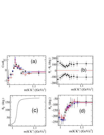
Figure 5: Results of the partial-wave analysis of the $K^{-}K^{+}$ system. (a) Cosine of relative phase $\theta_{SP}=\theta_{\textit{S}}-\theta_{P}$, (b) two solutions for $\theta_{SP}$, (c) P-wave phase for $\phi(1020)$, and (d) S-wave phase derived from the upper solution in (b). Solid bullets are data points, and open circles (blue) and open triangles (red) correspond, respectively, to isobar models I, II.

We find that two different isobar models describe the data well. Both yield almost identical behavior in invariant mass (Fig. 1b–1d) and angular distribution (Fig. 4). The dominance of $D^{0}\rightarrow K^{*+}K^{-}$ over $D^{0}\rightarrow K^{*-}K^{+}$ suggests that, in tree-level diagrams, the form factor for $D^{0}$ coupling to $K^{*-}$ is suppressed compared to the corresponding $K^{-}$ coupling. While the measured fit fraction for $D^{0}\rightarrow K^{*+}K^{-}$ agrees well with a phenomenological prediction theory based on a large SU(3) symmetry breaking, the corresponding results for $D^{0}\rightarrow K^{*-}K^{+}$ and the color-suppressed $D^{0}\rightarrow\phi\pi^{0}$ decays differ significantly. It appears from Table 1 that the $K^{+}\pi^{0}$ S-wave amplitude can absorb any $K^{*}(1410)$ and $f_{2}^{\prime}(1525)$ if those are not in the model. The other components are quite well established, independent of the model. From Table 1, the strong phase difference, $\delta_{D}$, between the $\kern 1.99997pt\overline{\kern-1.99997ptD}{}^{0}$ and $D^{0}$ decays to $K^{*}(892)^{+}K^{-}$ state and their amplitude ratio, $r_{D}$, are given by: $\delta_{D}$ = $-35.5^{\circ}\pm 1.9^{\circ}$ (stat) $\pm 2.2^{\circ}$ (syst) and $r_{D}$ = 0.599 $\pm$ 0.013 (stat) $\pm$ 0.011 (syst) mykkpi0 . Systematic uncertainties in quantities in Table 1 arise from experimental effects (e.g., efficiency parameters, background shape, particle-identification), and also from uncertainty in the nature of the models used to describe the data (e.g., $K\pi$ S-wave amplitude and resonance parameters).
We show the Legendre polynomials moments in Fig. 4 for the $K^{+}\pi^{0}$ and $K^{-}K^{+}$ channels, for $l=0-7$. We use the relations of Eq. 5 to evaluate $\left|S\right|$ and $\left|P\right|$ shown in Fig. 3, and $\theta_{\textit{SP}}$ shown in Fig. 5, for the $K^{-}K^{+}$ channel in the mass range $m_{K^{-}K^{+}}<1.15~{}{\mathrm{\,Ge\kern-1.00006ptV\!/}c^{2}}$. The measured values of $\left|S\right|$ agree well with those obtained in the analysis of the decay $D^{0}\rightarrow K^{-}K^{+}\bar{K^{0}}$ antimo and also with either the $f_{0}(980)$ or the $a_{0}(980)$ lineshape. The measured values of $\left|P\right|$ are consistent with a Breit-Wigner lineshape for $\phi(1020)$.

VI Dalitz plot analysis of $D^{0}\rightarrow\pi^{-}\pi^{+}\pi^{0}$

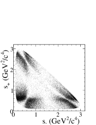
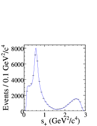
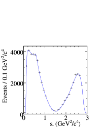
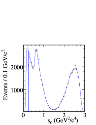
Figure 6: Dalitz plot and invariant mass-squared projections for the $D^{0}\rightarrow\pi^{-}\pi^{+}\pi^{0}$ decay excluding $D^{0}\rightarrow K_{s}^{0}\pi^{0}$.

An important component of the program to study $C\!P$ violation is the measurement of the angle $\gamma$ of the unitarity triangle related to the Cabibbo-Kobayashi-Maskawa quark mixing matrix. The decays $B\rightarrow D^{(*)0}K^{(*)}$ can be used to measure $\gamma$ with essentially no hadronic uncertainties, exploiting interference between $b\rightarrow u\overline{c}s$ and $b\rightarrow c\overline{u}s$ decay amplitudes. The most effective method to measure $\gamma$ has turned out to be the analysis of the $D$-decay Dalitz plot distribution in $B^{\pm}\rightarrow DK^{\pm}$ with multi-body $D$ decays ref:D . This method has only been used with the Cabibbo-favored decay $D\rightarrow K^{0}_{\scriptscriptstyle S}\pi^{+}\pi^{-}$ Abe:2003cn ; Aubert:2004kv . We perform the first $C\!P$-violation study of $B^{\pm}\rightarrow DK^{\pm}$ using a multibody, Cabibbo-suppressed $D$ decay, $D\rightarrow\pi^{+}\pi^{-}\pi^{0}$.

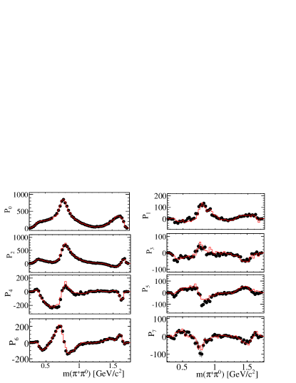
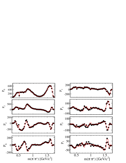
Figure 7: Legendre polynomials moments for the $\pi^{+}\pi^{0}$ (columns I, II) and $\pi^{-}\pi^{+}$ (columns III, IV) channels of $D^{0}\rightarrow\pi^{-}\pi^{+}\pi^{0}$. The circles with error bars are data points and the curves (red) are derived from the fit functions.

We determine the parameters $a_{r}$, $\phi_{r}$, and $f_{r}$ by fitting a large sample of $D^{0}$ and $\kern 1.99997pt\overline{\kern-1.99997ptD}{}^{0}$ mesons, flavor-tagged through their production in the decay $D^{*+}\rightarrow D^{0}\pi^{+}$ mybr . Of the $D$ candidates in the signal region $1848<m_{D^{0}}<1880$ ${\mathrm{\,Me\kern-1.00006ptV\!/}c^{2}}$, we obtain from the fit $44780\pm 250$ signal and $830\pm 70$ background events.

Table 2 summarizes the results of this fit, with systematic errors obtained by varying the masses and widths of the $\rho(1700)$ and $\sigma$ resonances and the form factors, and also varying the signal efficiency parameters to account for uncertainties in reconstruction and particle identification. The Dalitz plot distribution of the data is shown in Fig. 6(a-d). The distribution is marked by three destructively interfering $\rho\pi$ amplitudes, suggesting a final state dominated by $I=0$ ref:zemach . We show the Legendre polynomials moments in Fig. 7 for the $\pi^{+}\pi^{0}$ and $\pi^{-}\pi^{+}$ channels, for $l=0-7$. The agreement between data and fit is again excellent. Unlike in case of the decay $D^{0}\rightarrow K^{-}K^{+}\pi^{0}$, we cannot use the relations of Eq. 5 to evaluate $\left|S\right|$ and $\left|P\right|$, and $\theta_{\textit{SP}}$ in any of the two-body $\pi\pi$ channels because of the contributions from cross-channels in the entire available mass-range.

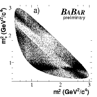
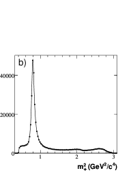
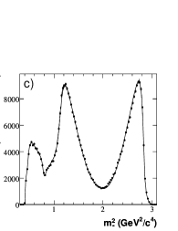
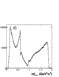
Figure 8: (a) The $\bar{D}^{0}\rightarrow K^{0}_{\scriptscriptstyle S}\pi^{-}\pi^{+}$ Dalitz distribution from $D^{*-}\rightarrow\bar{D}^{0}\pi^{-}$ events, and projections on (b) $m^{2}_{+}=m^{2}_{K^{0}_{\scriptscriptstyle S}\pi^{+}}$, (c) $m^{2}_{-}=m^{2}_{K^{0}_{\scriptscriptstyle S}\pi^{-}}$, and (d) $m^{2}_{\pi^{+}\pi^{-}}$. $D^{0}\rightarrow K^{0}_{\scriptscriptstyle S}\pi^{+}\pi^{-}$ from $D^{*+}\rightarrow D^{0}\pi^{+}$ events are also included. The curves are the model fit projections.

Figure 9: The invariant mass distribution of the reconstructed $D_{S}$ candidate in the decay $D_{s}^{+}\rightarrow K^{+}K^{-}\pi^{+}$. For the Dalitz plot analysis we use events in the mass window shown by vertical arrows. The results are preliminary.

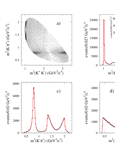
Figure 10: (a) The $D_{s}^{+}\rightarrow K^{+}K^{-}\pi^{+}$ Dalitz distribution, and projections on (b) $m^{2}_{K^{+}K^{-}}$, (c) $m^{2}_{K^{-}\pi^{+}}$, and (d) $m^{2}_{K^{+}\pi^{+}}$. The curves are the model fit projections. The results are preliminary.

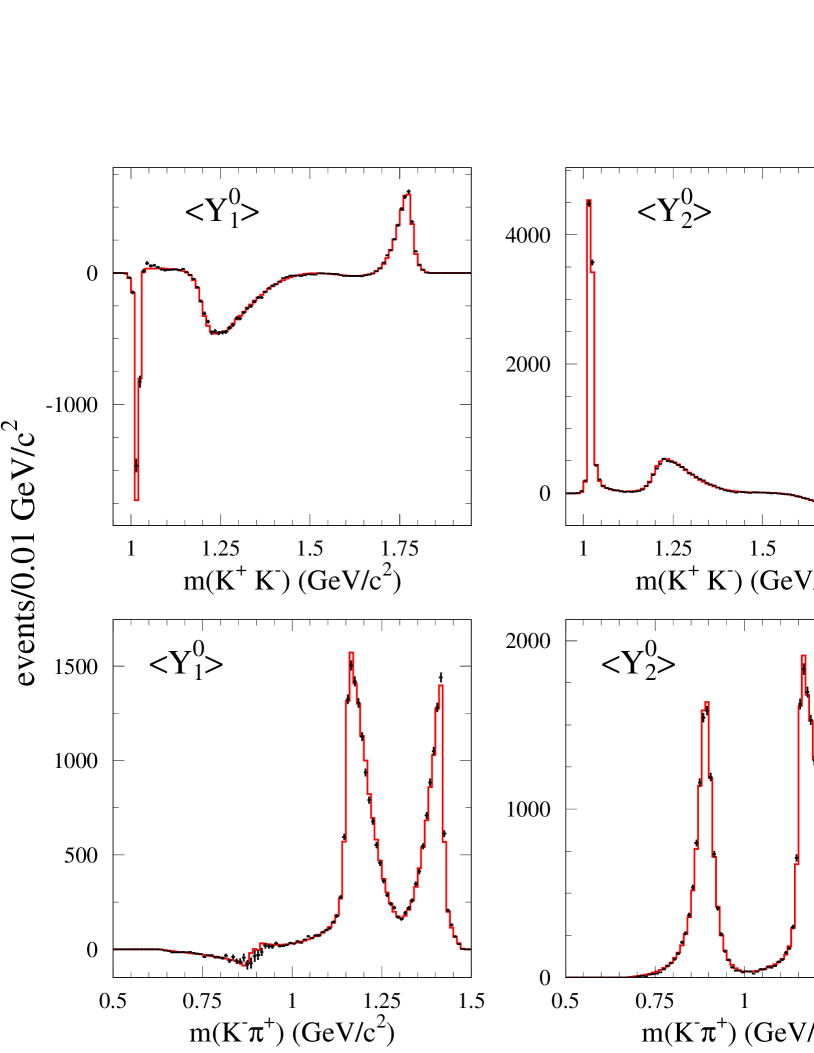
Figure 11: Legendre polynomials moments for the $K^{+}K^{-}$ (top) and $K^{-}\pi^{+}$ (bottom) channels of $D_{s}^{+}\rightarrow K^{+}K^{-}\pi^{+}$. The dots with error bars are data points and the curves are derived from the fit functions. The results are preliminary.

Table 2: The results obtained from the $D^{0}\rightarrow\pi^{-}\pi^{+}\pi^{0}$ Dalitz plot fit myGamma . The errors are statistical and systematic, respectively. We take the mass (width) of the $\sigma$ meson to be 400 (600) ${\mathrm{\,Me\kern-1.00006ptV\!/}c^{2}}$.

State	$a_{r}$ (%)	$\phi_{r}$ (∘)	$f_{r}(\%)$
$\rho(770)^{+}$	100	0	67.8$\pm$0.0$\pm$0.6
$\rho(770)^{0}$	58.8$\pm$0.6$\pm$0.2	16.2$\pm$0.6$\pm$0.4	26.2$\pm$0.5$\pm$1.1
$\rho(770)^{-}$	71.4$\pm$0.8$\pm$0.3	$-$2.0$\pm$0.6$\pm$0.6	34.6$\pm$0.8$\pm$0.3
$\rho(1450)^{+}$	21$\pm$6$\pm$13	$-$146$\pm$18$\pm$24	0.11$\pm$0.07$\pm$0.12
$\rho(1450)^{0}$	33$\pm$6$\pm$4	10$\pm$8$\pm$13	0.30$\pm$0.11$\pm$0.07
$\rho(1450)^{-}$	82$\pm$5$\pm$4	16$\pm$3$\pm$3	1.79$\pm$0.22$\pm$0.12
$\rho(1700)^{+}$	225$\pm$18$\pm$14	$-$17$\pm$2$\pm$3	4.1$\pm$0.7$\pm$0.7
$\rho(1700)^{0}$	251$\pm$15$\pm$13	$-$17$\pm$2$\pm$2	5.0$\pm$0.6$\pm$1.0
$\rho(1700)^{-}$	200$\pm$11$\pm$7	$-$50$\pm$3$\pm$3	3.2$\pm$0.4$\pm$0.6
$f_{0}(980)$	1.50$\pm$0.12$\pm$0.17	$-$59$\pm$5$\pm$4	0.25$\pm$0.04$\pm$0.04
$f_{0}(1370)$	6.3$\pm$0.9$\pm$0.9	156$\pm$9$\pm$6	0.37$\pm$0.11$\pm$0.09
$f_{0}(1500)$	5.8$\pm$0.6$\pm$0.6	12$\pm$9$\pm$4	0.39$\pm$0.08$\pm$0.07
$f_{0}(1710)$	11.2$\pm$1.4$\pm$1.7	51$\pm$8$\pm$7	0.31$\pm$0.07$\pm$0.08
$f_{2}(1270)$	104$\pm$3$\pm$21	$-$171$\pm$3$\pm$4	1.32$\pm$0.08$\pm$0.10
$\sigma(400)$	6.9$\pm$0.6$\pm$1.2	8$\pm$4$\pm$8	0.82$\pm$0.10$\pm$0.10
Non-Res	57$\pm$7$\pm$8	$-$11$\pm$4$\pm$2	0.84$\pm$0.21$\pm$0.12

VII Dalitz plot analysis of $D^{0}\rightarrow K^{0}_{\scriptscriptstyle S}\pi^{+}\pi^{-}$

The Dalitz plot analysis of the decay $D^{0}\rightarrow K^{0}_{\scriptscriptstyle S}\pi^{+}\pi^{-}$ is also motivated by its application to the measurement of CKM phase $\gamma$ babar_summer06 . We determine the $D^{0}\rightarrow K^{0}_{\scriptscriptstyle S}\pi^{+}\pi^{-}$ decay amplitude from an unbinned maximum-likelihood fit to the Dalitz plot distribution of a high-purity ($\sim 98\%$) $D^{0}$ sample from 390328 $D^{*+}\rightarrow D^{0}\pi^{+}$ decays reconstructed in 270 $\mbox{\,fb}^{-1}$ of data, shown in Fig. 8.

The decay amplitude is expressed as a coherent sum of two-body resonant terms and a uniform non-resonant contribution. For $r=\rho(770)$ and $\rho(1450)$ we use the functional form suggested in Ref. ref:gounarissakurai , while the remaining resonances are parameterized by a spin-dependent relativistic Breit-Wigner distribution. The model consists of 13 resonances leading to 16 two-body decay amplitudes and phases (see Table 3), plus the non-resonant contribution, and accounts for efficiency variations across the Dalitz plane and the small background contribution. All the resonances considered in this model are well established except for the two scalar $\pi\pi$ resonances, $\sigma$ and $\sigma^{\prime}$, whose masses and widths are obtained from our sample ref:comment_sigma . Their addition to the model is motivated by an improvement in the description of the data.

The possible absence of the $\sigma$ and $\sigma^{\prime}$ resonances is considered in the evaluation of the systematic errors. In this respect, the K-matrix formalism ref:Kmatrix provides a direct way of imposing the unitarity constraint that is not guaranteed in the case of the Breit-Wigner parametrization and is suited to the study of broad and overlapping resonances in multi-channel decays. We use the K-matrix method to parameterize the $\pi\pi$ S-wave states, avoiding the need to introduce the two $\sigma$ scalars. A description of this alternative parametrization can be found in Ref. ref:babar_dalitzeps05 .

Component	$Re\{a_{r}e^{i\phi_{r}}\}$	$Im\{a_{r}e^{i\phi_{r}}\}$	$f_{r}$ (%)
$K^{*}(892)^{-}$	$-1.223\pm 0.011$	$1.3461\pm 0.0096$	58.1
$K^{*}_{0}(1430)^{-}$	$-1.698\pm 0.022$	$-0.576\pm 0.024$	6.7
$K^{*}_{2}(1430)^{-}$	$-0.834\pm 0.021$	$0.931\pm 0.022$	6.3
$K^{*}(1410)^{-}$	$-0.248\pm 0.038$	$-0.108\pm 0.031$	0.1
$K^{*}(1680)^{-}$	$-1.285\pm 0.014$	$0.205\pm 0.013$	0.6
$K^{*}(892)^{+}$	$0.0997\pm 0.0036$	$-0.1271\pm 0.0034$	0.5
$K^{*}_{0}(1430)^{+}$	$-0.027\pm 0.016$	$-0.076\pm 0.017$	0.0
$K^{*}_{2}(1430)^{+}$	$0.019\pm 0.017$	$0.177\pm 0.018$	0.1
$\rho(770)$	$1$	$0$	21.6
$\omega(782)$	$-0.02194\pm 0.00099$	$0.03942\pm 0.00066$	0.7
$f_{2}(1270)$	$-0.699\pm 0.018$	$0.387\pm 0.018$	2.1
$\rho(1450)$	$0.253\pm 0.038$	$0.036\pm 0.055$	0.1
Non-res	$-0.99\pm 0.19$	$3.82\pm 0.13$	8.5
$f_{0}(980)$	$0.4465\pm 0.0057$	$0.2572\pm 0.0081$	6.4
$f_{0}(1370)$	$0.95\pm 0.11$	$-1.619\pm 0.011$	2.0
$\sigma$	$1.28\pm 0.02$	$0.273\pm 0.024$	7.6
$\sigma^{\prime}$	$0.290\pm 0.010$	$-0.0655\pm 0.0098$	0.9

Table 3: Complex amplitudes $a_{r}e^{i\phi_{r}}$ and fit fractions of the different components ($K_{S}\pi^{-}$, $K_{S}\pi^{+}$, and $\pi^{+}\pi^{-}$ resonances) obtained from the fit of the $D^{0}\rightarrow K_{S}\pi^{+}\pi^{-}$ Dalitz distribution from $D^{*+}\rightarrow D^{0}\pi^{+}$ events. Errors are statistical only.

VIII Dalitz plot analysis of $D_{s}^{+}\rightarrow K^{+}K^{-}\pi^{+}$

Decay Mode	Decay fraction(%)	Amplitude	Phase(radians)
$\bar{K}^{*}(892)^{0}K^{+}$	$48.7\pm 0.2\pm 1.6$	1.(Fixed)	0.(Fixed)
$\phi(1020)\pi^{+}$	$37.9\pm 0.2\pm 1.8$	$\quad 1.081\pm 0.006\pm 0.049$	$\quad 2.56\pm 0.02\pm 0.38$
$f_{0}(980)\pi^{+}$	$35\pm 1\pm 14$	$4.6\pm 0.1\pm 1.6$	$-1.04\pm 0.04\pm 0.48$
$\bar{K}^{*}_{0}(1430)^{0}K^{+}$	$2.0\pm 0.2\pm 3.3$	$1.07\pm 0.06\pm 0.73$	$-1.37\pm 0.05\pm 0.81$
$f_{0}(1710)\pi^{+}$	$2.0\pm 0.1\pm 1.0$	$0.83\pm 0.02\pm 0.18$	$-2.11\pm 0.05\pm 0.42$
$f_{0}(1370)\pi^{+}$	$6.3\pm 0.6\pm 4.8$	$1.74\pm 0.09\pm 1.05$	$-2.6\pm 0.1\pm 1.1$
$\bar{K}^{*}_{0}(1430)^{0}K^{+}$	$0.17\pm 0.05\pm 0.30$	$0.43\pm 0.05\pm 0.34$	$-2.5\pm 0.1\pm 0.3$
$f_{2}(1270)\pi^{+}$	$0.18\pm 0.03\pm 0.40$	$0.40\pm 0.04\pm 0.35$	$0.3\pm 0.2\pm 0.5$

Table 4: The results obtained from the $D_{s}^{+}\rightarrow K^{+}K^{-}\pi^{+}$ Dalitz plot fit, listing fit-fractions, amplitudes and phases. The errors are statistical and systematic, respectively. The results are preliminary.

We study the decay $D^{+}_{s}\rightarrow K^{+}K^{-}\pi^{+}$ using a data sample of 240 $\mbox{\,fb}^{-1}$. We focus particularly on the measurement of the relative decay rates ${{\cal{B}}(D^{+}_{s}\rightarrow\phi\pi^{+})}\over{{\cal{B}}(D^{+}_{s}\rightarrow K^{+}K^{-}\pi^{+})}$ and ${{\cal{B}}(D^{+}_{s}\rightarrow\bar{K}^{*0}(892)K^{+})}\over{{\cal{B}}(D^{+}_{s}\rightarrow K^{+}K^{-}\pi^{+})}$. The decay $D^{+}_{s}\rightarrow\phi(1020)\pi^{+}$ is frequently used as the $D^{+}_{s}$ reference decay mode. The improvement in the measurements of these ratios is therefore important. A previous Dalitz plot analysis of this decay used $\sim 700$ signal events e687 . We perform the present analysis using a number of signal events more than two orders of magnitude larger.

We reconstruct the decay by fitting the three charged tracks in the event to a common vertex, requiring the $\chi^{2}$ probability to be greater than 0.1%. We cleanly remove a small background from the decay $D^{*+}\rightarrow D^{0}_{K^{+}K^{-}}\pi^{+}$ by requiring $m_{K^{+}K^{-}}<1.85~{}{\mathrm{\,Ge\kern-1.00006ptV\!/}c^{2}}$. In Fig. 9 we show the invariant mass distribution of the reconstructed $D^{+}_{s}$ candidate in the decay $D_{s}^{+}\rightarrow K^{+}K^{-}\pi^{+}$. For the Dalitz plot analysis, we use events in the $\pm 2\sigma$ mass window of the reconstructed $D^{+}_{s}$ candidate. We parametrize the incoherent background shape empirically using the events in the sidebands. In the signal region, we find 100850 signal events with a purity of about 95%.

The Dalitz plot for the $D^{+}_{s}\rightarrow K^{+}K^{-}\pi^{+}$ events is shown in Fig. 10. In the $K^{+}K^{-}$ threshold region, a strong $\phi(1020)$ signal can be observed, together with a rather broad structure indicating the presence of the $f_{0}(980)$ and $a_{0}(980)$ S-wave resonances. A strong $K^{*0}(890)$ signal can also be seen. We perform an unbinned maximum likelihood fit to determine the relative amplitudes and phases of intermediate resonant and non-resonant states. The complex amplitude coefficient for each of the contributing states is measured with respect to $\overline{K}{}^{*0}K^{+}$. We summarize the fit results in Table 4 showing fit-fractions, amplitudes, and phases of the contributing resonances. The projections of the Dalitz plot variables in data and the ones from the fit results are shown in Fig. 10. Further tests on the fit quality can be estimated using $Y^{0}_{L}$ angular moments. These moments are shown for the $K^{+}K^{-}$ and $K^{-}\pi^{+}$ channels in Fig. 11. The agreement between the data and fit is excellent. We find a rather large contribution from the $f_{0}(980)\pi^{+}$, but with a large systematic uncertainty due primarily to a poor knowledge of the shape parameters of $f_{0}(980)$ and higher $f_{0}$ states.

From the fit-fraction values reported in Table 4, we make the following preliminary measurements:

${{\cal{B}}(D^{+}_{s}\rightarrow\phi\pi^{+})}\over{{\cal{B}}(D^{+}_{s}\rightarrow K^{+}K^{-}\pi^{+})}$ $=$ 0.379 $\pm$ 0.002 (stat) $\pm$ 0.018 (syst),

${{\cal{B}}(D^{+}_{s}\rightarrow\bar{K}^{*0}(892)K^{+})}\over{{\cal{B}}(D^{+}_{s}\rightarrow K^{+}K^{-}\pi^{+})}$ $=$ 0.487 $\pm$ 0.002 (stat) $\pm$ 0.016 (syst).

IX Conclusions

we have studied the amplitudes of the decays $D^{0}\rightarrow K^{-}K^{+}\pi^{0}$, $D^{0}\rightarrow\pi^{-}\pi^{+}\pi^{0}$, $D^{0}\rightarrow K^{0}_{\scriptscriptstyle S}\pi^{+}\pi^{-}$, and $D_{s}^{+}\rightarrow K^{+}K^{-}\pi^{+}$. Using $D^{0}\rightarrow K^{-}K^{+}\pi^{0}$ Dalitz plot analysis, we measure the strong phase difference between the $\kern 1.99997pt\overline{\kern-1.99997ptD}{}^{0}$ and $D^{0}$ decays to $K^{*}(892)^{+}K^{-}$ and their amplitude ratio, which will be useful in the measurement of the CKM phase $\gamma$. We observe contributions from the $K\pi$ and $K^{-}K^{+}$ scalar and vector amplitudes, and analyze their angular moments. We find no evidence for charged $\kappa$, nor for higher spin states. We also perform a partial-wave analysis of the $K^{-}K^{+}$ system in a limited mass range. We measure the magnitudes and phases of the components of the $D^{0}\rightarrow\pi^{+}\pi^{-}\pi^{0}$ decay amplitude, which we use in constraining the CKM phase $\gamma$ using $B^{\pm}\rightarrow D_{\pi^{+}\pi^{-}\pi^{0}}K^{\pm}$. We measure the amplitudes of the neutral $D$-meson decays to the $K^{0}_{s}\pi^{-}\pi^{+}$ final state and use the results as input in the measurement of $\gamma$ using the decay $B^{\mp}\rightarrow D^{(*)}_{K^{0}_{s}\pi^{-}\pi^{+}}K^{\mp}$. Finally we parametrize the amplitudes of the $D_{s}^{+}\rightarrow K^{+}K^{-}\pi^{+}$ Dalitz plot and perform precision measurements of the relative decay rates ${{\cal{B}}(D^{+}_{s}\rightarrow\phi\pi^{+})}\over{{\cal{B}}(D^{+}_{s}\rightarrow K^{+}K^{-}\pi^{+})}$ and ${{\cal{B}}(D^{+}_{s}\rightarrow\bar{K}^{*0}(892)K^{+})}\over{{\cal{B}}(D^{+}_{s}\rightarrow K^{+}K^{-}\pi^{+})}$.

X Acknowledgements

We are grateful for the excellent luminosity and machine conditions provided by our PEP-II colleagues, and for the substantial dedicated effort from the computing organizations that support BABAR. This work is supported by the United States Department of Energy and National Science Foundation.

References

(1)
B. Aubert et al. (BABAR Collaboration), hep-ex/0703037, accepted
for publication in Phys. Rev. Lett.
(2)
B. Aubert et al. (BABAR Collaboration), Nucl. Instr. and
Methods A479, 1 (2002).
(3)
W. -M. Yao et al. (PDG), J. Phys. , 1 (2006).
(4)
J.M. Blatt and W.F. Weisskopf, Theoretical Nuclear Physics, John Wiley
& Sons, New York, 1952.
(5)
Reference to the charge-conjugate decay is implied throughout. The initial
state referred to is , not .
(6)
E.M. Aitala et al. (E-791 Collaboration), Phys. Rev. Lett. 89, 121801 (2002).
(7)
B. Aubert et al. (BABAR Collaboration), Phys. Rev. D74, 091102 (2006).
(8)
D. Aston et al. (LASS Collaboration), Nucl. Phys. B296,
493 (1988); W.M. Dunwoodie, private communication.
(9)
B. Aubert et al. (BABAR Collaboration),
Phys. Rev. D76, 011102 (R)(2007).