Constraints on the Magnetic Field Geometry of Magnetars

Abstract

We study the effect of the magnetic field geometry on the oscillation spectra of strongly magnetized stars. We construct a configuration of magnetic field where a toroidal component is added to the standard poloidal one. We consider a star with a type I superconductor core so that both components of the magnetic field are expelled from the core and confined in the crust. Our results show that the toroidal contribution does not influence significantly the torsional oscillations of the crust. On the contrary, the confinement of the magnetic field in the crust drastically affects on the torsional oscillation spectrum. Comparison with estimations for the magnetic field strength, from observations, exclude the possibility that magnetars will have a magnetic field solely confined in the crust i.e. our results suggest that the magnetic field in whatever geometry has to permeate the whole star.

1 Introduction

It is known that magnetic fields play important role in the astrophysical phenomena, such as supernovae, gamma-ray bursts, galaxy jet, and so on. Recently, there is a growing consensus in explaining Soft Gamma Repeaters (SGRs) via the magnetar model (Duncan & Thompson, 1992). Magnetars are believed to be neutron stars with strong magnetic field which is responsible for the observed flare activity. Three giant flares, SGR 0526-66, SGR 1900+14, and SGR 1806-20, have been detected so far. The peak luminosities are in the range of $\simeq 10^{44}-10^{46}$ erg/s. This huge amounts of energy can be explained by the presence of a strong magnetic field whose strength is estimated to be larger than $4\times 10^{14}$ Gauss for SGR 1900+14 (Hurley et al., 1999) and of the order of $8\times 10^{14}$ Gauss for SGR 1806-20 (Kouveliotou et al., 1998). In addition to the initial short and hard peak, these three events show a decaying tail lasting hundreds of seconds. In this late part careful analysis revealed the existence of characteristic Quasi Periodic Oscillations (QPOs); see Strohmayer & Watts (2006) for references. The oscillation frequencies in these QPOs are in the range of a few tenths of Hz to kHz and thought to be associated with crust torsional modes of magnetars. These signals might be the first evidence of a direct detection of crust oscillations of neutron stars: a first attempt to explain these frequencies by the crust torsional oscillations has been done by using a model with dipole magnetic fields and realistic EoS (see Samuelsson & Andersson (2007) and Sotani et al. (2007a)) and this attempt was partially successful. On the other hand Glampedakis et al. (2006) suggested an alternative scenario to explain the observational frequencies via Alfvén oscillations while Levin (2006) was the first to realize that the Alfvén oscillations of magnetars could be a continuum. More recently Levin (2007) pointed out that the edges or turning point of the continuum can be long-lived QPOs. In a recent paper, Sotani et al. (2007b) showed that the Alfvén oscillations of magnetars could be a continuum which can explain the lower ones of the observed frequencies.

However, it is quite difficult to construct realistic models for neutron star magnetic fields and/or to understand the details of their dynamics. In fact, the observational data suggest that the surface temperature of neutron stars with a strong magnetic field is not uniform (e.g., Showpe et al. (2005); Haberl et al. (2006)). This observational evidence can be explained, for example, by the presence of magnetic fields in the crust region with a strong toroidal components or a more complicated structure than the poloidal one (Geppert et al., 2006; Pons & Geppert, 2007). Such crustal magnetic fields can be generated if the core is a type I superconductor. In this case, the magnetic fields are expelled from the core due to the Meissner effect after about $10^{4}$ years .

Recently, the analysis of the spectrum of timing noise for SGR 1806-20 and SGR 1900+14 has supported the idea that the core region can be a type II superconductor (Arras et al., 2004). For the type II superconductor, even if an initial uniform magnetic field is present in the core, it will be split in thin magnetic fluxes tubes (fluxoids), which are parallel to the initial magnetic field. These fluxoids interact with the neutron vortices and are driven by these vortices outside the core, towards the crust on a timescale of $10^{8}-10^{9}$ years (Ruderman, 2005). In any case, it is too difficult to discriminate between all these models by using only the past observational data. This is due to uncertainties associated with the chemical composition of the interior and the crust of neutron stars as well as about the interior magnetic field configuration and its influence on the properties of neutron star.

The aim of this paper is to calculate the axisymmetric crust torsional modes of magnetars with both poloidal and toroidal magnetic field, where both the components are confined in the crust. Then our numerical results show that this magnetic configuration cannot explain the actual observational data of SGRs. In this paper, we adopt the unit of $c=G=1$, where $c$ and $G$ denote the speed of light and the gravitational constant, respectively, and the metric signature is $(-,+,+,+)$.

2 Equilibrium Configuration

The deformation from spherical symmetry due to the magnetic pressure would be small, because the magnetic energy is considerably smaller than the gravitational energy. So in this paper we neglect the effect of deformations induced by the magnetic field as well as the rotational deformations since the known magnetars rotate slowly. For these reasons, the equilibrium model of neutron stars can be described by a spherically symmetric solutions of the Tolman-Oppenheimer-Volkov (TOV) equations. The line element is given then by

$$ds^{2}=-e^{2\Phi}dt^{2}+e^{2\Lambda}dr^{2}+r^{2}(d\theta^{2}+\sin^{2}\theta d\phi^{2}),$$ (1)

and the 4-velocity is expressed as $u^{\mu}=(e^{-\Phi},0,0,0)$. In the following, we assume an ideal MHD approximation and we consider an axisymmetric magnetic field generated by a 4-current $J^{\mu}$. In order to determine the distribution of magnetic fields we need two basic relations: the Maxwell equations and the equation of motions that can be obtained by projecting the conservation of the energy-momentum tensor $T^{\mu\nu}$ on to the hypersurface normal to $u^{\mu}$ (see equation (11) in Sotani et al. (2007a)). These two equations are:

$$F^{\mu\nu}_{\ \ ;\nu} = 4\pi J^{\mu},$$ (2)

$$(\epsilon+p)u^{\nu}u_{\mu;\nu}+p_{,\mu}+u_{\mu}u^{\nu}p_{,\nu} = F_{\mu\nu}J^{\nu},$$ (3)

where $F_{\mu\nu}$ is the Faraday tensor linked to the electromagnetic 4-potential $A_{\mu}$ by $F_{\mu\nu}=A_{\nu,\mu}-A_{\mu,\nu}$. With the appropriate gauge condition, we can set $A_{\mu}$ as

$$A_{\mu}=(0,A_{r},0,A_{\phi}).$$ (4)

With $J^{r}$ and $J^{\theta}$ obtained from the equation (2), the equation (3) for $\mu\equiv\phi$ can be written as

$$\tilde{A}_{r,\theta}A_{\phi,r}-\tilde{A}_{r,r}A_{\phi,\theta}=0,$$ (5)

where $\tilde{A}_{r}$ is defined as $\tilde{A}_{r}\equiv e^{\Phi-\Lambda}A_{r,\theta}\sin\theta$. Thus $\tilde{A}_{r}$ depends on $A_{\phi}$ and we can set $\tilde{A}_{r}=\zeta A_{\phi}$ (where $\zeta$ is a constant, see below for its meaning) since $\tilde{A}_{r}$ is of the same order as $A_{\phi}$ with respect to the magnetic field strength. If we expand $A_{\phi}$ as

$$A_{\phi}=a_{\ell_{M}}(r)\sin\theta\partial_{\theta}P_{\ell_{M}}(\cos\theta),$$ (6)

then, the 4-potential $A_{\mu}$ has the form

$$A_{\mu}=(0,\zeta e^{-\Phi+\Lambda}a_{\ell_{M}}P_{\ell_{M}},0,a_{\ell_{M}}\sin\theta\partial_{\theta}P_{\ell_{M}}).$$ (7)

In the following, we will consider only dipole fields i.e. $\ell_{M}=1$.

In order to obtain an expression for the 4-current $J^{\mu}$, we can get additional equations from the equation (3) by setting $\mu\equiv r,\theta$:

$$\chi_{,r}=A_{\phi,r}\tilde{J}_{\phi}\ \ \ \mbox{and}\ \ \ \chi_{,\theta}=A_{\phi,\theta}\tilde{J}_{\phi},$$ (8)

where $\chi$ is a function of $r$ and $\theta$ and

$$\tilde{J}_{\phi} \equiv \frac{1}{r^{2}\sin^{2}\theta(\epsilon+p)}\left[J_{\phi}-\frac{\zeta^{2}}{4\pi}e^{-2\Phi}A_{\phi}\right],$$ (9)

$$\chi_{,r} \equiv C_{s}^{2}(\ln n)^{\prime}+\Phi^{\prime}.$$ (10)

Note that $C_{s}$ is the sound speed, while in order to derive the above equations we have used the first law of thermodynamics, i.e, $d\epsilon=(\epsilon+p)dn/n$, where $n$ is the number density of particles. Using the integrability condition $\chi_{,r\theta}=\chi_{,\theta r}$ together with equation (8), we obtain $A_{\phi,r}\tilde{J}_{\phi,\theta}-A_{\phi,\theta}\tilde{J}_{\phi,r}=0$. Thus we can see that $\tilde{J}_{\phi}$ is also function of $A_{\phi}$ and it is possible to rewrite $\tilde{J}_{\phi}$ as $\tilde{J}_{\phi}=-f_{0}-f_{1}A_{\phi}$, where $f_{0}$ and $f_{1}$ are some constants. Comparing this last expression with equation (9), we get the following expression for $J_{\phi}$:

$$J_{\phi}=\frac{\zeta^{2}}{4\pi}e^{-2\Phi}A_{\phi}-(f_{0}+f_{1}A_{\phi})(\epsilon+p)r^{2}\sin^{2}\theta.$$ (11)

For simplicity we neglect the contribution of $f_{1}$ .

Setting $\mu\equiv\phi$ in Maxwell equations (2) and by making use of equation (11) we derive the following equation for $a_{1}$

$$e^{-2\Lambda}\frac{d^{2}a_{1}}{dr^{2}}+(\Phi^{\prime}-\Lambda^{\prime})e^{-2\Lambda}\frac{da_{1}}{dr}+\left(\zeta^{2}e^{-2\Phi}-\frac{2}{r^{2}}\right)a_{1}=-4\pi j_{1},$$ (12)

where $j_{1}=f_{0}r^{2}(\epsilon+p)$. For the exterior region, if we assume only dipole magnetic fields, i.e., $\zeta=0$, there is an analytic solution for $a_{1}^{\rm{(ex)}}$ that is:

$$a_{1}^{\rm{(ex)}}=-\frac{3\mu_{b}r^{2}}{8M^{3}}\left[\ln\left(1-\frac{2M}{r}\right)+\frac{2M}{r}+\frac{2M^{2}}{r^{2}}\right],$$ (13)

where $\mu_{b}$ is the magnetic dipole moment observed at infinity. The interior solution for $a_{1}$ should be determined by solving numerically equation (12) and requiring that $a_{1}$ and ${a_{1}}^{\prime}$ are continuous across the stellar surface. Hence, the components of the vector $H_{\mu}\equiv B_{\mu}/\sqrt{4\pi}$, are given by

$$H_{r} = \frac{e^{\Lambda}a_{1}}{\sqrt{\pi}r^{2}}\cos\theta,$$ (14)

$$H_{\theta} = -\frac{e^{-\Lambda}{a_{1}}^{\prime}}{\sqrt{4\pi}}\sin\theta,$$ (15)

$$H_{\phi} = -\frac{\zeta e^{-\Phi}a_{1}}{\sqrt{4\pi}}\sin\theta.$$ (16)

¿From these expressions, we can see that the parameter $\zeta$ is a constant associated only with the toroidal component of the magnetic field. Additionally the value of $\zeta$ is chosen in the range where the function of $a_{1}$ has no node inside the star. Therefore there exists a maximum value of $\zeta$ named as $\zeta_{max}$. Note that we can produce magnetar models with larger value of $\zeta$ than $\zeta_{max}$. But for these models, the structure of the magnetic field becomes more complex since the sign of current is not constant in the star, and this could lead to possible instability of the magnetic fields. In other words, when the sign of current changes, even if the star remains stable the magnetic field structure might undergo a catastrophic instability which will restructure the field. So we examine only the magnetar models with $\zeta\leq\zeta_{max}$.

In this paper we consider a stellar model with a superfluid core (type I superconductor) so that the magnetic field is expelled from the core by the Meissner effect. As a consequence, the magnetic fields are confined only in the crust region. In order to construct the model, we have to impose the condition that the magnetic fields are vanishing inside the core, i.e., we require that $a_{1}$ should be zero at the basis of crust. This condition can be written as $a_{1}\simeq\alpha_{c}(r-R_{c})$, where $\alpha_{c}$ is a constant and $R_{c}$ is the radius at the basis of the crust. Note that at $r=R_{c}$ both $H_{r}$ and $H_{\phi}$ vanish while $H_{\theta}$ is not zero. In Figure 1, we plot the components of magnetic field, where $\tilde{H}_{r}$, $\tilde{H}_{\theta}$, and $\tilde{H}_{\phi}$ are defined as $\tilde{H}_{r}\equiv R^{3}H_{r}/\mu_{b}$, $\tilde{H}_{\theta}\equiv R^{2}H_{\theta}/\mu_{b}$, and $\tilde{H}_{\phi}\equiv R^{2}H_{\phi}/\mu_{b}$. The actual details of the used stellar models will be described in the next section. It is worth noticing, from these figures, that the $\theta$ components of magnetic fields are not smooth at the stellar surface, because we assume an exterior magnetic field with only a poloidal component, which means $\zeta=0$ for $r\geq R$ i.e. no toroidal component outside the star. This choice produces a current on the star surface. The presence of a surface current is found also in many simulations dealing with the evolution and the stability of the magnetic field (see Braithwaite & Spruit (2006)). Howevere we do not consider the existence of the surface current in this paper, since the surface current dose not affect the behavior of the torsional oscillations within our analysis.

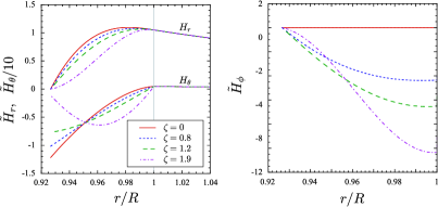
Figure 1: The three components, ${\tilde{H}}_{r}\equiv R^{3}H_{r}/\mu_{b}$ (for $\theta=0$), ${\tilde{H}}_{\theta}\equiv R^{2}H_{\theta}/\mu_{b}$ (for $\theta=\pi/2$) and ${\tilde{H}}_{\phi}\equiv R^{2}H_{\phi}/\mu_{b}$ (for $\theta=\pi/2$) of the magnetic field for a stellar model with $1.4M_{\odot}$. The different lines correspond to different values of the constant $\zeta$ with $\zeta_{max}=1.9$. Note also that ${\tilde{H}}_{\theta}$ is scaled by a factor ten.

3 Numerical results

In this paper, we adopted polytropic equations of state (EoS) described by the following relations

$$p=Kn_{0}m_{b}\left(\frac{n}{n_{0}}\right)^{\Gamma}\ \mbox{and}\ \ \ \rho=nm_{b}+\frac{p}{\Gamma-1},$$ (17)

where $m_{b}=1.66\times 10^{-24}$ g and $n_{0}=0.1$ fm^-3, and we have set $\Gamma=2.46$ and $K=0.00936$ by fitting the tabulated data for EoS A (Pandharipande, 1971). With this equation of state and with the fixed value of the density at $r=R_{c}$, $\rho=2.4\times 10^{14}$ g/cm³, the maximum mass is $M_{max}\simeq 1.654M_{\odot}$. Here we study two representative stellar models; one with $M=1.4M_{\odot}$ and the other is the one with the maximum allowed mass for this EoS i.e. the one with $M=1.654M_{\odot}$. For these two stellar models, the radius, the relative crust thickness, and the compactness are $R=10.35$ km, $\Delta r/R=7.34$ %, and $M/R=0.200$ for the model with $M=1.4M_{\odot}$ while the model with $M=1.654M_{\odot}$ has $R=8.95$ km, $\Delta r/R=4.15$ %, and $M/R=0.273$. Finally, for simplicity the shear modulus in the crust, $\mu$, is assumed to be given by a relation of the formula $\mu=v_{s}^{2}\rho$, where $v_{s}$ is the speed of shear waves with a typical value $v_{s}\simeq 10^{8}$ cm/s (Schumaker & Thorne, 1983). In general the frequencies of torsional oscillations depend on the EoS in the crust region since the shear modulus also depend on the EoS. However, in Sotani et al. (2007a) we have used two different realistic EoS for the crust and our results show that the freuqencies of fundamental torsional oscillations are almost independent of them. Anyway in this paper, as first approximation, we use the above simple formula for shear modulus.

We study axial perturbations in the Cowling approximation of the previous stellar models. We focus only on these type of oscillations of the crust (torsional) since they do not induce density perturbations, which means that significantly lower energy is needed for their excitation. On the other hand the absence of density perturbations leads to minimal metric perturbations which justifies our choice in using the Cowling approximation. Under these assumptions the perturbation equations are reduced to equation (51) in Sotani et al. (2007a). By studying this equation one can observe that, if the background magnetic fields are axisymmetric, the axisymmetric torsional oscillations are independent from the component $H_{\phi}$ of the magnetic field. Thus we can calculate the eigen-frequencies by using the perturbation equations (69) and (70) in Sotani et al. (2007a) with exactly the same boundary conditions, such as ${\cal Y}_{,r}=0$ at the basis of crust ($r=R_{c}$) and at the stellar surface ($r=R$), where ${\cal Y}(r)$ describes the angular displacement of the stellar material. However, we have to replace $j_{1}$ in equation (70) in Sotani et al. (2007a) by $\tilde{j}_{1}=j_{1}+\zeta^{2}e^{-2\Phi}a_{1}/(4\pi)$, because for the elimination of the term of ${a_{1}}^{\prime\prime}$ we have used equation (12).

The numerical results are shown in Figure 2, where the fundamental $\ell=2$ torsional modes are plotted as function of the normalized magnetic field $B/B_{\mu}$ ($B_{\mu}=4\times 10^{15}$ Gauss). ¿From these figures, it is clear that the frequencies depend weakly on the presence of the toroidal magnetic fields, even if the strength of the toroidal field increases i.e. the value of $\zeta$ becomes larger. This weak dependence can be understood if we recall that the magnetic field lines of the toroidal component are parallel to the direction of fluid motion. But the most important result is that, although it seems that qualitatively the effect of the magnetic field is similar to the results in Sotani et al. (2007a), there is a significant quantitative difference: the influence of the magnetic field on the axisymmetric torsional frequencies becomes apparent for considerably lower strengths of the magnetic field, i.e. already for $B/B_{\mu}\approx 0.1$. Notice that the results in Sotani et al. (2007a) show that the effect of the magnetic field can be seen for $B/B_{\mu}\,\raisebox{-3.44444pt}{$\stackrel{{\scriptstyle\textstyle>}}{{\sim}}$ }1$. It is natural that when the magnetic field is confined in the crust, magnetic field becomes considerably stronger than the one that permeates the whole star for the same strength of the exterior magnetic field. Actually, since the magnetic field is confined in the crust which has thickness $\Delta r\sim 0.03-0.12R\approx 0.5-1.5$km, the density of magnetic field lines becomes higher. Also if we compare the results for the two stellar models under discussion we observe that thinner is the crust, then earlier the effect of the magnetic field becomes pronounced. For example, for the model with $M=1.654M_{\odot}$ ($\Delta r/R=4.15$ %) the effect of magnetic field is apparent for $B/B_{\mu}\approx 0.07$. For the other model ($M=1.4M_{\odot}$ and $\Delta r/R=7.34$ %) the effect of the magnetic field becomes pronounced later, i.e., $B/B_{\mu}\approx 0.1$.

The above results are derived by using the same procedure as in Sotani et al. (2007a), i.e. we decompose the system into spherical harmonics and truncate the ($\ell\pm 2$) terms. This truncation could introduce small errors in the results, thus in order to check the validity of our results we have used an alternative technique based on 2D numerical evolutions of the perturbation equation describing the dynamics of the oscillating crust. The 2D method used here is similar to the one described in Sotani et al. (2007b) and the evolution equations were structurally similar although the various background terms have been modified to include terms related to the shear modulus, $\mu$. The 2D evolution was constrained only in the crust and in the first quadrant i.e. $0\leq\theta\leq\pi/2$ and the following boundary conditions have been imposed: (a) ${\cal Y}_{,r}=0$ at $r=R_{c}$ and $R$, (b) ${\cal Y}_{,\theta}=0$ at $\theta=0$, and (c) ${\cal Y}=0$ at $\theta=\pi/2$. The results of the two approaches for $\zeta=0$ are plotted in in Figure 3. The continuous line corresponds to results derived by using the truncated equations and treating the problem as a boundary value one while the thick dots correspond to results produced by the 2D numerical evolution. The agreement between the two approaches is apparent, which suggests that for this type of problems the truncation of the ($\ell\pm 2$) equations does not affect at all the results.

Furthermore, we performed similar calculations for stellar models with different realistic EoS, but the behavior of frequencies, as function of a magnetic field, is similar to that for the EoS A that we use here.

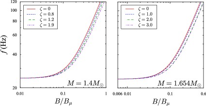
Figure 2: With $M=1.4M_{\odot}$ and $1.654M_{\odot}$, the frequencies of the fundamental torsional modes of $\ell=2$ as functions of $B/B_{\mu}$, where $B_{\mu}=4\times 10^{15}$ Gauss. The different lines correspond to different values of $\zeta$, where $\zeta_{max}\sim 1.9$ for $M=1.4M_{\odot}$ and $\zeta_{max}\sim 3.0$ for $M=1.654M_{\odot}$.

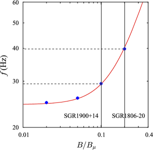
Figure 3: The torsional mode frequencies as functions of the magnetic field strength for $\zeta=0$. The continuous line shows the results from the 1-D truncated mode calculation on which we omitted the coupling to $\ell\pm 2$ equations while the thick dots correspond to results from 2D numerical evolutions of the perturbation equations. In this figure two vertical lines has been drawn corresponding to the estimated magnetic field strengths for the two SGRs that is $B\approx 4\times 10^{14}$ Gauss for SGR 1900+14 and $B\approx 8\times 10^{14}$ Gauss for SGR 1806-20.

4 Constraints on the Magnetic Field Geometry

We have studied the torsional oscillations for the magnetic field distribution where the magnetic fields has been “expelled” from the superfluid core and confined in the crust. We have also assumed that the magnetic field has both poloidal and toroidal components. The study shows that the presence of the toroidal field affects marginally the oscillation frequencies of the torsional modes, which can be explained because the perturbations propagate along the toroidal field lines. The toroidal field might play a more significant role in the case of non-axisymmetric perturbations or if we include the coupling to polar perturbations.

The main results of this work is summarized in Figure 3. Our calculations show that the effect of magnetic field on the torsional modes, when it is confined only in the crust, can be observed for magnetic field strengths below $10^{14}$ Gauss. Moreover, this observation has a significant effect on understanding the geometry of the magnetic field of magnetars. The reason is the following. With this magnetic field configuration there are no additional oscillational frequencies such as Alfvén oscillations (see Sotani et al. (2007b)), because the magnetic field does not exist in the core. Thus the $\ell=2$ torsional oscillation is lowest oscillational frequency. On the other hand the estimated magnetic field strengths are of the order of a few times $10^{14}$ Gauss (Hurley et al., 1999; Kouveliotou et al., 1998) or even higher (Nakagawa et al., 2007). This suggest that if the magnetic field was constrained to the crust the lowest possible frequency for the signals from SGR 1806-20 is about 40 Hz. Then, this magnetic field distribution can not explain the observed frequencies 18, 26 and 29 Hz. So this type of magnetic field geometry cannot be present in the observed magnetars and most probably it has to be excluded in general for the case of strongly magnetized neutron stars. Alternative scenarios which might include coupling with the polar modes should be excluded since crustal perturbations of polar type are typically of considerably higher frequencies (Strohmayer, 1991; Vavoulidis et al., 2007) and cannot explain all three frequencies.

Appendix A Poloidal and toroidal fields permeating the star

In this appendix we study the effect on the torsional mode spectrum of the toroidal component added on the poloidal magnetic field configuration studied in Sotani et al. (2007a). In this case the magnetic field permeates the whole star but we study only the oscillations of the crustal part of the star. Although this is somehow a truncation of the full problem, it may be a good approximation in studying the effect of the toroidal component (see the next paragraph for an argument in favour of this). Following Sotani et al. (2007a), the equilibrium configuration of the magnetic field is constructed by imposing the regularity condition, $a_{1}\simeq\alpha_{c}r^{2}$, at the stellar center, and by requiring the continuity of $a_{1}$ with the analytic exterior solution (13). The contribution of the toroidal field is set to zero for $r\geq R$. The components of the magnetic field are plotted in Figure 4 in a similar fashion as in Figure 1.

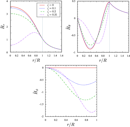
Figure 4: The three components, ${\tilde{H}}_{r}\equiv R^{3}H_{r}/\mu_{b}$ (for $\theta=0$), ${\tilde{H}}_{\theta}\equiv R^{2}H_{\theta}/\mu_{b}$ (for $\theta=\pi/2$) and ${\tilde{H}}_{\phi}\equiv R^{2}H_{\phi}/\mu_{b}$ (for $\theta=\pi/2$) of the magnetic field for a stellar model with $1.4M_{\odot}$. The different lines correspond to different values of the constant $\zeta$ with $\zeta_{max}=0.31$.

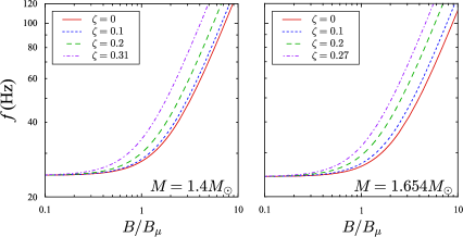
Figure 5: The frequencies of the fundamental torsional modes with $\ell=2$ as functions of $B/B_{\mu}$ with $M=1.4M_{\odot}$ and $1.654M_{\odot}$. The different lines correspond to different values of $\zeta$, where $\zeta_{max}\sim 0.31$ for $M=1.4M_{\odot}$ and $\zeta_{max}\sim 0.27$ for $M=1.654M_{\odot}$.

The torsional oscillation frequencies are calculated following the same procedure as in Sotani et al. (2007a), i.e., 1-D truncated mode calculation using the same boundary conditions, i.e., ${\cal Y}_{,r}=0$ at $r=R_{c}$ and $r=R$. Actually, the boundary condition at $r=R_{c}$ is not quite correct because in this way we ignore the coupling with the fluid core (Sotani et al., 2007c). Thus the proper boundary condition is $H^{r}H_{r}{\cal Y}^{(-)}_{,r}=\left[\mu+H^{r}H_{r}\right]{\cal Y}^{(+)}_{,r}$, which can be written as ${\cal Y}^{(+)}_{,r}/{\cal Y}^{(-)}_{,r}\approx\beta^{2}/(\beta^{2}+1)$, where $\beta=B/B_{\mu}$. ¿From this relation it is evident that for magnetic fields with strength around $B/B_{\mu}\simeq 0.1-0.3$ the coupling with the fluid core is not so important for the study of pure crust torsional oscillations. The corrections to our approximate boundary condition arise only for $B/B_{\mu}\,\raisebox{-3.44444pt}{$\stackrel{{\scriptstyle\textstyle>}}{{\sim}}$ }1$. Thus approximately we adopt the simple boundary condition ${\cal Y}_{,r}=0$ at the basis of crust, which will be used to demonstrate the effect of the toroidal component on the spectrum of torsional oscillations.

In Figure 5 we show the frequencies of the fundamental $\ell=2$ torsional modes as function of the normalized magnetic field strengh, $B/B_{\mu}$. As mentioned in Sotani et al. (2007a), the effect of magnetic field on torsional modes becomes important for $B\sim B_{\mu}$. This is expected since for $B>B_{\mu}$ the Alfvén speed, $u_{A}\equiv B/(4\pi\rho)^{1/2}$, becomes larger than the shear speed, $u_{s}\equiv(\mu/\rho)^{1/2}$. ¿From these figures, it is clear that the presence of the toroidal magnetic field affects weakly the frequencies of the torsional oscillations.

Concluding, the presence of a toroidal magnetic field component does not affect significantly the spectrum of the crust oscillations neither in the case when the poloidal field permeates the star nor when it is confined in the crust. This suggests that although we are able to exclude the presence of crust confined magnetic fields in magnetars, most probably we will not be able via the QPOs observations to identify the presence of a toroidal component in the magnetic field.

References

- Arras et al. (2004) Arras P., Cumming A., Thompson C., 2004, ApJ, 608, L49
- Braithwaite & Spruit (2006) Braithwaite J., Spruit H.C., 2006, A&A, 450, 1097
- Duncan & Thompson (1992) Duncan R.C, Thompson C., 1992, ApJ, 392, L9
- Geppert et al. (2006) Geppert U., Küker M., Page D., 2006, A&A, 457, 937
- Glampedakis & Andersson (2006) Glampedakis K., Andersson N., 2006, Phys. Rev. D, 74, 044040
- Glampedakis et al. (2006) Glampedakis K., Samuelsson L., Andersson N., 2006, MNRAS, 371, L74
- Haberl et al. (2006) Haberl F., Turolla R., de Vries C., 2006, A&A, 441, 597
- Hurley et al. (1999) Hurley K., et al., 1999, Nature, 397, L41
- Konno et al. (1999) Konno K., Obata T., Kojima Y., 1999, A&A, 352, 211
- Kouveliotou et al. (1998) Kouveliotou C., et al., 1998, Nature, 393, L235
- Levin (2006) Levin Y., 2006, MNRAS, 368, L35
- Levin (2007) Levin Y., 2006, MNRAS, 377, 159
- Nakagawa et al. (2007) Nakagawa Y.E., Yoshida A., Yamaoka K., preprint (astro-ph/0710.3816)
- Pandharipande (1971) Pandharipande V.R., 1971, Nucl. Phys. A, 178, 123
- Pons & Geppert (2007) Pons J.A., Geppert U., preprint (astro-ph/0703267)
- Ruderman (2005) Ruderman M., preprint (astro-ph/0510623)
- Samuelsson & Andersson (2007) Samuelsson L., Andersson N., 2007, MNRAS, 374, 256
- Schumaker & Thorne (1983) Schumaker B.L., Thorne K.S., 1983, MNRAS, 203, 457
- Sedrakian & Cordes (1998) Sedrakian A., Cordes J.M., 1998, ApJ, 502, 378
- Showpe et al. (2005) Showpe A., et. al., 2005, A&A, 441, 597
- Sotani et al. (2007a) Sotani H., Kokkotas K.D., Stergioulas N., 2007a, MNRAS, 375, 261
- Sotani et al. (2007b) Sotani H., Kokkotas K.D., Stergioulas N., 2007b MNRAS in press (astro-ph/0710.1113)
- Sotani et al. (2007c) Sotani H., Kokkotas K.D., Stergioulas N., Vavoulidis M., 2007c preprint (astro-ph/0611666).
- Strohmayer (1991) Stohmayer T.E., 1991, ApJ, 372, 573
- Strohmayer & Watts (2006) Stohmayer T.E., Watts A.L., 2006, ApJ, 653, 593
- Vavoulidis et al. (2007) Vavoulidis M., Kokkotas K.D., Stavridis A., MNRAS in press (gr-qc/0712.1263)