Controlling spatiotemporal chaos in excitable media using an array of control points

Abstract

The dynamics of activation waves in excitable media can give rise to spiral turbulence, the resulting spatiotemporal chaos being associated with empirical biological phenomena such as life-threatening disturbances in the natural rhythm of the heart. In this paper, we propose a spatially extended but non-global scheme using an array of control points for terminating such spatiotemporally chaotic excitations. A low-amplitude control signal is applied sequentially at each point on the array, resulting in a traveling wave of excitation in the underlying medium which drives away the turbulent activity. Our method is robust even in the presence of significant heterogeneities in the medium, which have often been an impediment to the success of other control schemes.

Excitable media are a class of models for a wide range of physical, chemical and biological systems that show spontaneous formation of spatial patterns, such as spiral waves Keener . These spiral waves, under certain conditions, may become unstable and break up, giving rise to spatiotemporal chaos. Such phenomena have been seen to occur in a large variety of natural systems described by excitable media, e.g., through interactions between chemical concentration waves in the Belusov-Zhabotinsky reaction Zaik70 and CO oxidation on Pt(110) surface Jaku90 , cyclic AMP waves involved in the organization of multicellular morphogenesis in Dictyostelium Sieg95 , intracellular calcium waves in Xenopus oocytes Lech91 , intercellular calcium waves in brain slices Harr98 ; Huan04 , and propagating electrical activity in the pregnant uterus Lamm97 and cardiac tissue Gray98 ; Witk98 . The last example is of particular importance as spatiotemporally varying patterns of excitation have been implicated in clinically significant disturbances of the natural rhythm of the heart, which are termed as arrhythmias. In fibrillation, a potentially life-threatening arrhythmia, there is complete loss of coordination between different regions of the heart due to spatially extended chaotic activity Winfree . The resulting cessation in the mechanical pumping action necessary for blood circulation, can lead to death within minutes unless the condition is terminated promptly. Conventional defibrillation is done by applying a large electrical shock across the heart, which is not only extremely painful, but can also damage cardiac tissue. Thus, devising a low-amplitude control method for spatiotemporal chaos in excitable media is an exciting challenge, as well as, having potential clinical relevance Christini01 ; Gauthier02 ; Pumir07 .

Low-amplitude control of chaos in excitable media needs to take into account certain special features of such systems, which hinder the straightforward application of methods successful in other chaotic systems. In particular, there exists a threshold for the stimulation, only on exceeding which excitation occurs as indicated by a characteristic action potential. Thus, the control signal amplitude needs to be above a lower bound to effect discernible changes in the medium, ruling out simple proportional feedback schemes. The other complicating factor is the existence of a recovery period immediately following excitation, during which the medium will not respond to a normal supra-threshold stimulus. This implies that two excitation wavefronts will annihilate on collision, as neither can penetrate the other, their wavebacks being in the recovery phase. This recovery period is distinguished into absolute, during which the cell is insensitive to any perturbation, and relative, when a larger than normal stimulus can excite the cell, the amplitude depending on the exact phase of recovery. Therefore, the amplitude and timing of the control signal needs to be appropriately chosen, so that it results in a response from the medium. Note that, the excited state is metastable, and the cell eventually recovers to the resting state associated in different biological systems with a characteristic resting transmembrane potential ($\simeq-84$ mV for cardiac myocyte cells). Thus, the control of spatiotemporal chaos in excitable media is essentially a problem of synchronizing the excitation phase of every cell, so that the entire system returns to the resting state, resulting in the termination of all activity.

Chaos control schemes for excitable media may be broadly classified into Sinha06 : (i) global, where the control signal is applied to all points of the system, (ii) local, where only a small localized region of the system is subject to control, and (iii) spatially extended but non-global schemes. Non-global methods use less power and also are relatively easier to implement practically, needing fewer control points. However, strictly local control methods almost always involve very high-frequency stimulation Zhang05 , that can by itself lead to reentrant waves in the presence of inhomogeneities PanfK93 ; Shajahan . Moreover, the effect of local stimulation at a point can affect the rest of the system only through diffusion. As wavefronts annihilate on collision, control-induced waves are restricted to the local neighborhood of the stimulation point during spiral turbulence, with the existing excited fragments closer to the control point shielding chaotic activity further away. By using a spatially extended but non-global scheme Sinha01 one can potentially avoid these drawbacks. In this paper, we terminate chaos in excitable media by applying spatiotemporally varying stimulation along an array of control points. The control signal appears to propagate along the array, triggering an excitation wavefront in the underlying medium, that is regenerated after each collision with chaotic fragments and in the process eliminating all existing activity. Stimulating each point once (or at most, twice) is seen to successfully control chaos in almost all instances. Although an array of control points have been used earlier to prevent the breakup of a single spiral Rappel99 , to the best of our knowledge this is the first instance showing control of fully developed spatiotemporal chaos in excitable media using only a finite number of control points without repeated stimulations at high frequency.

The spatiotemporal dynamics of excitation in several biological systems can be described by:

$$\partial{V}/\partial{t}=\frac{-I_{ion}+I_{ext}(x,y,t)}{C_{m}}+D\nabla^{2}V,$$ (1)

where $V$ (mV) is the transmembrane potential, $C_{m}$ = 1 $\mu$F cm^-2 is the transmembrane capacitance, $D$ (cm²s^-1) is the diffusion constant, $I_{ion}$ ($\mu$A cm^-2) is the transmembrane ionic current density and $I_{ext}(x,y,t)$ is the space- and time-dependent external stimulus current density applied for control on a 2-dimensional surface. For the specific functional form of $I_{ion}$, we used the Luo-Rudy I (LR1) action potential model Luo , where, it is assumed to be composed of six distinct currents, each of them being determined by several time-dependent ion-channel gating variables $\xi$ whose time-evolution is described by differential equations $\frac{d\xi}{dt}=\frac{\xi_{\infty}-\xi}{\tau_{\xi}}$. The parameters in these equations are the steady-state values of $\xi$, $\xi_{\infty}=\alpha_{\xi}/(\alpha_{\xi}+\beta_{\xi})$, and the time constants, $\tau_{\xi}=1/(\alpha_{\xi}+\beta_{\xi})$, which are governed by the voltage-dependent rate constants for the opening and closing of the channels, $\alpha_{\xi}$ and $\beta_{\xi}$, themselves complicated functions of $V$. In order to verify the model independence of our results and to carry out three-dimensional simulations, we have also used a simpler description of the action potential, as given by Panfilov (PV) Panfilov93 ; Panfilov98 : $I_{ion}=f(V)-g$, where $f$ is a piecewise linear approximation of a cubic function and $g$ is an effective membrane conductance evolving with time as $\frac{dg}{dt}=\epsilon(V,g)(kV-g)$. The time-constant $\epsilon$ is a function of both $V$ and $g$ and the parameters used are same as that in Ref. Sinha01 . The models are solved using a forward-Euler scheme, the system being discretized on a spatial grid with spacing $\delta x$ (=0.0225 cm for LR1, = 0.05 cm for PV). The simulation domain is a square lattice of $L\times L$ points in two dimensions or a cuboid with $L\times L\times L_{z}$ points in three dimensions. For the LR1 simulations, $L$ = 400, while for PV, $L$ = 256 (for 2-d) and $L=128,L_{z}=8$ (for 3-d). The standard five-point and seven-point difference stencils are used for the Laplacian in two and three dimensions, respectively. The time step for integration is chosen to be $\delta t$ = 0.01 ms (for LR1) and = 0.11 ms (for PV). No-flux boundary conditions are implemented at the edges of the simulation domain. The initial spatiotemporally chaotic state is obtained by creating a broken wavefront which evolves into a spiral wave and is then allowed to become unstable, eventually breaking up into multiple wavelets (in LR1 this process takes, on average, 200 ms).

We now focus on the control term $I_{ext}(x,y,t)$. For a 2-d domain of size $L\times L$ we consider

$$I_{ext}=I(x,y,t)\delta(x-md)\delta(y-nd),$$ (2)

where, the delta function is defined as $\delta(z)=1$ if $z=0$, and $=0$, otherwise, $d$ is the spatial interval between points in an array where the control signal is applied and $m,n$ are integers in the interval $[0,L/d]$. The current density $I(x,y,t)=I_{0}$ for $t\in[\sqrt{x^{2}+y^{2}}/v,(\sqrt{x^{2}+y^{2}}/v)+\tau]$, and $=0$ otherwise, corresponds to a rectangular control pulse of amplitude $I_{0}$ of duration $\tau$ that is travelling with velocity $v$. At the onset of control ($t=0$), the point at $(0,0)$ is stimulated, followed a short duration later by the points at $(0,d)$ and $(d,0)$, and this process continues as the control pulse proceeds like a traveling wave across the array. At each control point, the stimulation may excite the underlying region depending on its recovery phase. An excited region can in turn spread the effect of the stimulation to the surrounding regions through diffusion. Fig. 1 shows this process of secondary wave generation at the stimulated control points, creating a sustained excitation wavefront. Note that, any portion of this stimulated wavefront in the medium that is broken through collision with chaotic fragments, can be regenerated by subsequent control points. Hence, there is effectively an unbroken wavefront that travels through the medium, sweeping away the spatiotemporal chaos and leaving the system in a recovering state. As each control point needs to impose order over a region of size $\sim d^{2}$ to eliminate spatiotemporal chaos, this highlights the critical role of $d$. Indeed, for large $v$, the method approaches global control as $d\rightarrow 0$, while for $d\sim L$ the control stimulation is confined to a single, localized region. This implies that as $d$ increases, terminating chaos becomes increasingly difficult. For example, in LR1 model, chaos control fails for $d\geq 13$.

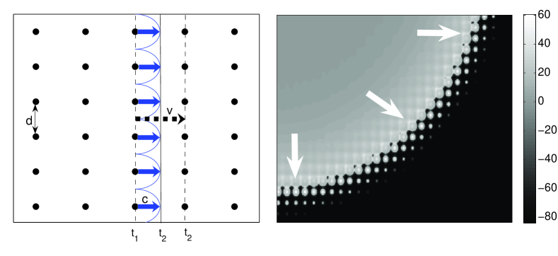
Figure 1: (left) Schematic diagram and (right) pseudo-gray-scale plot of the transmembrane potential $V$ for the two-dimensional LR1 model, showing the propagation of the control-induced excitation wavefront. The control signal traveling with velocity $v$ stimulates at time $t_{1}$ a column of points (spaced $d$ apart) from which secondary excitations traveling with velocity $c$ are generated. At time $t_{2}$ the control signal stimulates the next column of points, which the induced excitation wave may or may not have reached depending on the relative values of $v$ and $c$ [$v/c=4$ in (right)].

Before reporting the simulation results, we consider the role played by the traveling wave nature of the control pulse. The success of the proposed method depends on the control signal velocity, $v$, relative to the velocity of the excitation wavefront propagating via diffusion, $c$ (= 60.75 cm s^-1 for LR-1, = 50.9 cm s^-1 for PV, for the parameters used here). When $v\rightarrow 0$, the control method reduces to a local scheme regardless of $d$, as the effect of the external stimulation can only propagate in the system via diffusion. On the other hand, when $v$ is very large, all the control points are stimulated almost simultaneously. While the traveling wave nature of the control pulse allows propagation of stimulation independent of diffusion through the excitable medium, for $v\simeq c$ the excitation propagating by diffusion reinforces the external stimulation at each control point. Further, for a control signal propagating with a finite velocity (thus engaging only a few points at any given time), the energy applied per unit time to the medium is much lower than that for simultaneous stimulation of all the control points (i.e., $v\rightarrow\infty$).

For a system undergoing chaotic activity, the medium will at any time be at an extremely heterogeneous state, with certain regions excited and other regions partially or fully recovered. The vital condition for successful termination of chaos is that after the passage of the control-stimulated wave there should not remain any unexcited region which is partially recovered and can be subsequently activated by diffusion from a decaying excitation front. This places a lower bound on the control signal parameters, i.e., the signal amplitude $I_{0}$ and its duration $\tau$. If either is decreased below this bound, the external stimulation is unable to excite certain partially recovered regions. If these regions have neighboring chaotic fragments, whose activity is slowly decaying after collision with the control-induced wave, then, there will be a diffusion current from the latter. Depending on the phase of recovery, this may be sufficient to stimulate activity in the partially recovered regions, thereby re-initiating spatiotemporal chaos after the control signal has passed through.

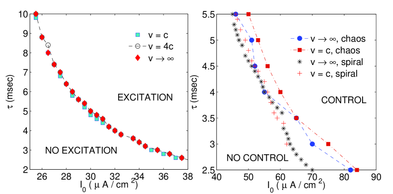
Figure 2: Strength-duration curves for LR1 model (in a two-dimensional domain with $L=400$) when control stimulation is applied on (left) quiescent homogeneous medium and (right) medium with existing excitation activity, either a single spiral or spatiotemporal chaos. In both figures, control is applied over a grid of points which are spaced apart by $d=10$. Different curves correspond to different control signal velocities $v$, relative to $c$, the excitation wavefront velocity in the medium. For values of $I_{0}$ and $\tau$ above the curves, the external stimulation results in (left) excitation of the domain or (right) control of existing activity.

To understand in detail the lower bound on the external stimulation parameters $I_{0}$ and $\tau$, we first look at the condition for exciting a completely homogeneous medium in the resting state. The stimulation at each point must exceed the local threshold in order to generate an action potential. This could be achieved either directly through an external current $I_{ext}$ or indirectly through diffusion from a neighboring excited region. Fig. 2 (left) shows the result of applying control signals with different $I_{0}$ and $\tau$ at points which are spaced a distance $d$ apart. The resulting strength-duration curve Gedd70 ; Gold97 indicates that the response of the system is not sensitively dependent on the propagation velocity $v$ of the control signal along the grid. As $d$ decreases, excitation is possible at lower values of $I_{0}$ and $\tau$, the minimum being for the case when all points are subject to direct external stimulation ($d\rightarrow 0$). This is because the entire applied current $I_{0}$ at any point is used to raise its state above the threshold, no part being lost to neighboring regions through diffusion.

For systems with existing activity, such as self-sustaining spiral waves or spatiotemporal chaos, the regions in the relative recovery period can be excited by stimuli larger than that needed for a fully recovered medium. Hence, the strength-duration curve for control of such a system will shift towards higher values of $I_{0}$ and $\tau$ (Fig. 2, right). We observe that the minimum external stimulus required for control does not vary significantly if the medium is undergoing fully developed spatiotemporal chaos as opposed to having a single spiral wave. Further, the velocity of the control signal along the array is not critical to the success in eliminating existing activity, provided $v$ is not significantly smaller than $c$. Note that, if $v$ is sufficiently small or $d$ increases beyond a critical value, the control fails, as the effect of the control signal is confined to the region immediately surrounding the stimulated point.

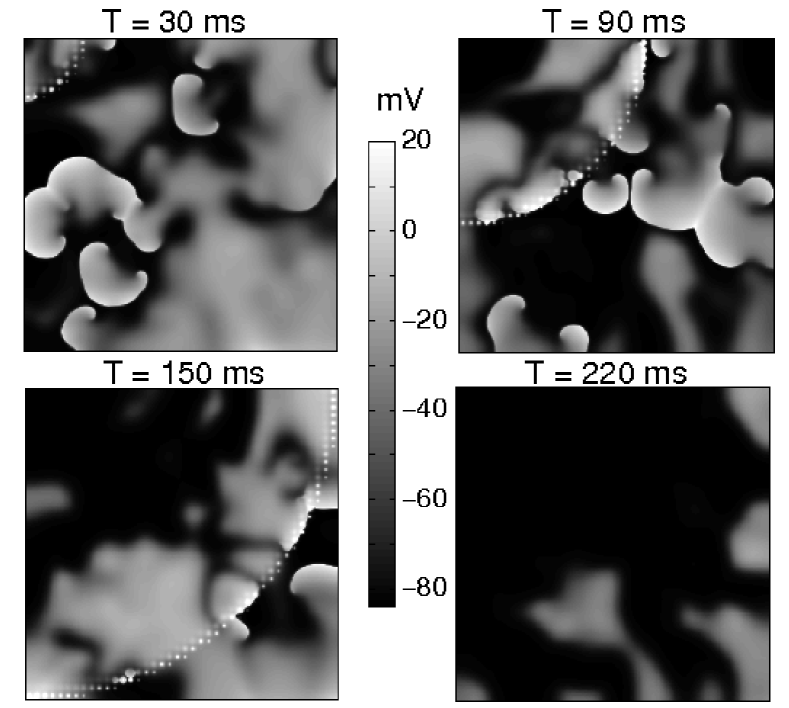
Figure 3: Pseudo-gray-scale plots of the transmembrane potential $V$ for the two-dimensional LR1 model ($L=400$) showing the elimination of all chaotic activity within 300 ms after initiation of control. A single wave of control stimulus ($I_{0}=75$ $\mu$A/cm², $\tau=3$ ms) begins at the top left corner ($T=0$) and travels across the domain with velocity $v=c$. This results in stimulating the region around the control points (spaced apart by $d=10$) in a sequential manner, creating a stimulated wavefront seen as an arc consisting of excited points in the panels above.

Fig. 3 shows the successful termination of spatiotemporal chaos in the LR1 model using a control signal that travels across the 2-dimensional domain while exciting points in the medium that are spaced apart by $d=10$. We verified that the control scheme is not model dependent by using it to eliminate spatiotemporal chaotic activity in the PV model. As most systems in reality have depth, it is crucial to verify that the method is successful in controlling chaos in a 3-dimensional domain, even when the external stimulus is applied only on one surface. This latter restriction follows from the fact that, in most practical situations it may not be possible (or desirable) to penetrate the medium physically in order to apply control signals inside the bulk. We confirmed that our method works in thin slices of excitable media of size $L\times L\times L_{z}$ ($L_{z}\ll L$), when the array of control points is placed on one of the $L\times L$ surfaces (Fig. 4). Even in cases where a single control-stimulated wave across the medium is unable to terminate all activity, we notice that it results in driving the chaotic activity further towards the boundaries and away from the origin of control stimulation. Thus, using multiple waves through application of control signals at intervals which are larger than the recovery period of the medium, the chaos in the bulk of 3-dimensional systems is successfully terminated.

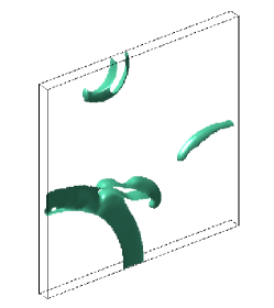
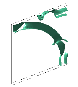
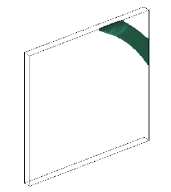
Figure 4: The effect of applying control on a single surface of a 3-dimensional domain using the PV model ($L$ = 128 and $L_{z}=8$). Two waves of control signal ($I_{0}=10$, $\tau=16.5$ ms, $v=c$) are applied 165 ms apart resulting in termination of spatiotemporal chaos. The interval between control points, $d\rightarrow 0$. The panels show isosurface plots at $T=242$ ms (left), 308 ms (center) and 341 ms (right).

We have checked that small distortions in the regular array of control points does not result in the failure of our method. Similarly, starting the control signal at different points of origin (and indeed, using a planar wave rather than a curved wave) does not affect the efficacy of the scheme. Further, our method is robust in the presence of conduction inhomogeneities (such as inexcitable obstacles) that tend to destabilise local control schemes. Fig. 5 shows successful control of chaos when the medium contains a large region of slow conduction, i.e., an extremely small value of $D$ compared to the rest of the medium.

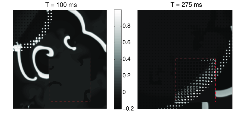
Figure 5: Pseudo-gray-scale plots of the transmembrane potential $V$ for the two-dimensional PV model ($L=256$) showing chaos control in the presence of a conduction inhomogeneity (of size $110\times 110$, indicated by the broken lines). Inside this region, $D_{inhomogen}=0.01D$, the diffusion constant of the rest of the medium. A single pulse of control stimulus ($I_{0}=8$, $\tau=17$ ms, $v=c$) is applied over an array of control points spaced apart by $d=8$, resulting in termination of all activity by $T=350$ ms.

In this paper, we have presented a novel control scheme involving external stimulation applied over an array of points, that is successful in terminating spatiotemporal chaos in both simplified as well as realistic models of biological excitable media. The control signal amplitude is varied both spatially and temporally, such that it appears as a propagating wave along the array of control points. This results in a stimulated wavefront in the excitable medium, that, depending on the propagation velocity of the control signal and the space interval between control points, eliminates all existing activity. Our method requires very low-amplitude control currents applied for short durations at a finite number of points, each point being stimulated once (or at most, twice) in most situations. Further, it is successful in terminating chaos in the bulk of a three-dimensional medium even when applied only on one surface. The use of significantly lower number of control points than that necessary for global control methods, makes the proposed scheme more suitable for practical implementation.

We thank the IMSc Complex Systems Project and IFCPAR (Project 3404-4) for financial support.

References

- (1) J. Keener and J. Sneyd, Mathematical Physiology (Springer, New York, 1998).
- (2) A.N. Zaikin and A.M. Zhabotinsky, Nature (London) 225, 535 (1970).
- (3) S. Jakubith, H.H. Rotermund, W. Engel, A. von Oertzen and G. Ertl, Phys. Rev. Lett. 65, 3013 (1990).
- (4) F. Siegert and C.J. Weijer, Curr. Biol. 5, 937 (1995).
- (5) J. Lechleiter, S. Girard, E. Peralta and D. Clapham, Science 252, 123 (1991).
- (6) M.E. Harris-White, S.A,. Zanotti, S.A. Frautschy and A.C. Charles, J. Neurophysiol. 79, 1045 (1998).
- (7) X. Huang, W.C. Troy, Q. Yang, H. Ma, C.R. Laing, S.J. Schiff and J.-Y. Wu, J. Neurosci. 24, 9897 (2004).
- (8) W.J.E.P. Lammers, Pflügers Arch. 433, 287 (1997).
- (9) R.A. Gray, A.M. Pertsov and J. Jalife, Nature (London) 392, 75 (1998).
- (10) F.X. Witkowski, L.J. Leon, P.A. Penkoske, W.R. Giles, M.L. Spano, W.L. Ditto and A.T. Winfree, Nature (London) 392, 78 (1998).
- (11) A.T. Winfree, When Time Breaks Down (Princeton University Press, Princeton, NJ, 1987).
- (12) D.J. Christini, K.M. Stein, S.M. Markowitz, S. Mittal, D.J. Slotwiner, M.A. Scheiner, S. Iwai and B.B. Lerman, Proc. Natl. Acad. Sci. USA 98, 5827 (2001).
- (13) D.J. Gauthier, G.M. Hall, R.A. Oliver, E.G. Dixon-Tulloch, P.D. Wolf and S. Bahar, Chaos 12, 952 (2002).
- (14) A. Pumir, V. Nikolski, M. Hörning, A. Isomura, K. Agladze, K. Yoshikawa, R. Gilmour, E. Bodenschatz and V. Krinsky, Phys. Rev. Lett., in press.
- (15) S. Sinha and S.Sridhar, in Handbook of Chaos Control (Eds. E. Schöll and H-G. Schuster) Weinheim: Wiley-VCH Verlag, 2007. (also at arxiv:0710.2265)
- (16) H. Zhang, Z. Cao, N.J. Wu, P.H. Ying and G. Hu, Phys. Rev. Lett. 94, 188301 (2005).
- (17) A.V. Panfilov and J.P. Keener, J. Theor. Biol. 163, 439 (1993).
- (18) T.K. Shajahan et al, to be published.
- (19) S. Sinha, A. Pande and R. Pandit, Phys. Rev. Lett. 86, 3678 (2001).
- (20) W-J Rappel, F. Fenton and A. Karma, Phys. Rev. Lett. 83, 456 (1999).
- (21) C.H. Luo and Y.Rudy, Circ.Res 68, 1501 (1991).
- (22) A.V. Panfilov and P. Hogeweg, Phys. Lett. A 176, 211 (1993).
- (23) A.V. Panfilov, Chaos 8, 57 (1998).
- (24) L.A. Geddes, W.A. Tacker, J. Mcfarlane and J. Bourland, Circ. Res. 27, 551 (1970).
- (25) M.R. Gold and S.R. Shorofsky, Circulation 96, 3517 (1997).