Theoretical study on isotopic shift in angle-resolved photoemission spectra of Bi₂Sr₂CaCu₂O₈

Abstract

We develop a path-integral theory to study the angle-resolved photoemission spectra (ARPES) of high-$T_{c}$ superconductors based on a two-dimensional model for the CuO₂ conduction plane, including both electron-electron ($e$-$e$) and electron-phonon ($e$-ph) interactions. Comparing our result with the experimental one of Bi₂Sr₂CaCu₂O₈, we find that the experimentally observed isotopic band shift in ARPES is due to the off-diagonal quadratic $e$-ph coupling, whereas the presence of $e$-$e$ repulsion partially suppresses this effect.

1 Introduction

The study of high-$T_{c}$ superconductivity is one of the most attractive realms in the last two decades. Since the angle-resolved photoemission spectroscopy (ARPES) directly probes the electronic occupied states, it has become an important technique to investigate the electronic properties of cuprates[1]. Recently, the oxygen isotope effect has been detected with ARPES in Bi₂Sr₂CaCu₂O₈ (Bi2212) by two groups[2, 3], and a common feature is noticed that the spectra are shifted with the ¹⁶O/¹⁸O substitution, providing direct evidence for electron-phonon ($e$-ph) coupling in this material. However, since the first report by Gweon et al.[2], this isotopic band shift has become an controversial issue[4], as the observed shift is up to 40 meV, much larger than the isotopic energy change of oxygen phonon, $\sim$ 5 meV[5]. Very recently, Douglas et al.[3] repeat the experiment, but find the shift is only 2$\pm$3 meV. Thus it turns out to be an interesting problem whether the large shift observed by Gweon et al. is possible or not in the cuprates. In this paper we shall look into this isotope induced band shift from a theoretical point of view.

In the CuO₂ plane of cuprates, as shown in Fig. 1, the electronic transfer is affected by the vibration of oxygen atoms between the initial and final Cu sites, resulting in an off-diagonal type $e$-ph coupling. In order to have an insight into the isotope effect of Bi2212, we start from a half-filled Hamiltonian including the electron-electron ($e$-$e$) repulsion and the above mentioned off-diagonal $e$-ph coupling ($\hbar=1$ and $k_{B}=1$ throughout this paper):

$$H = -\sum_{\langle l,l^{\prime}\rangle,\sigma}t(l,l^{\prime})(a^{{\dagger}}_{l\sigma}a_{l^{\prime}\sigma}+a^{{\dagger}}_{l^{\prime}\sigma}a_{l\sigma})+U\sum_{l}n_{l\uparrow}n_{l\downarrow}+{\omega_{0}\over 2}\sum_{\langle l,l^{\prime}\rangle}\left(-{1\over\lambda}\frac{\partial^{2}}{\partial q^{2}_{ll^{\prime}}}+q^{2}_{ll^{\prime}}\right),$$ (1)

where $a^{{\dagger}}_{l\sigma}$ ($a_{l\sigma}$) is the creation (annihilation) operator of an electron with spin $\sigma$ at the Cu site $l$ on a square lattice (see in Fig. 1). The electrons hop between two nearest neighboring Cu sites, denoted by $\langle l,l^{\prime}\rangle$, with a transfer energy $t(l,l^{\prime})$. $U$ is the strength of Coulomb repulsion between two electrons on the same Cu site with opposite spins. The oxygen phonon is assumed to be of the Einstein type with a frequency $\omega_{0}$ and a mass $m$. $\lambda$ ($\equiv 1+\Delta m/m$) is the mass change factor of phonon due to the isotope substitution. In the third term, $q_{ll^{\prime}}$ is the dimensionless coordinate operator of the oxygen phonon locating between the nearest-neighboring Cu sites $l$ and $l^{\prime}$, and the sum denoted by ${\langle l,l^{\prime}\rangle}$ just means a summation over all the phonon sites in the lattice.

Figure 1: A Schematic plot of CuO₂ conduction plane in cuprates. The copper atom (white circle) is on the $l$-th site of a simple square lattice. The oxygen atom (black circle) is located between the nearest-neighboring Cu sites, and $q_{ll^{\prime}}$ denotes its displacement from the equilibrium position.

In the conduction plane of CuO₂, the electronic hopping integral $t(l,l^{\prime})$ can be expanded to the second order terms with respect to the phonon displacements $q_{ll^{\prime}}$ as

$$t(l,l^{\prime})=t_{0}+sq^{2}_{ll^{\prime}},$$ (2)

where $t_{0}$ is the bare hopping energy and $s$ the off-diagonal quadratic $e$-ph coupling constant. Here we note the linear $e$-ph coupling does not occur owing to the lattice symmetry of present model. Whereas the inter-site $e$-$e$ interaction is included in the screened values of $t_{0}$ and $s$.

2 Path-integral Monte Carlo

In this section, we develop a path-integral theory for a model with both $e$-$e$ and $e$-ph interactions. By making use of the Trotter’s decoupling formula, the Boltzmann operator is written as,

$$e^{-\beta H}=\lim_{L\rightarrow\infty}\left(e^{-\Delta H}\cdots e^{-\Delta H}\right).$$ (3)

Applying the Hubbard-Stratonovitch transformation[6] and the Gaussian integral formula[7], we decouple the two-body parts, so that the $e$-$e$ and $e$-ph correlated terms are replaced by a two-fold summation over the auxiliary spin and lattice configurations, which is the so-called path-integral. In this way, the Boltzmann operator is rewritten into the path-integral form as,

$$e^{-\beta H} \rightarrow \int{\mathcal{D}}x\left(T_{+}\exp\left\{-\int_{0}^{\beta}d\tau\left[h(\tau,x_{m},x_{q})+\Omega(x_{q})\right]\right\}\prod_{l}\left[|x_{q}(l,\theta)\rangle\langle x_{q}(l,0)|\right]\right),$$ (4)

$$h(\tau,x_{m},x_{q}) \equiv -\sum_{\langle l,l^{\prime}\rangle,\sigma}\left[t_{0}+sx^{2}_{q}(l,l^{\prime},\tau)\right]\left[a^{{\dagger}}_{l\sigma}(\tau)a_{l^{\prime}\sigma}(\tau)+a^{{\dagger}}_{l^{\prime}\sigma}(\tau)a_{l\sigma}(\tau)\right]$$ (5)

$$-\sqrt{U\over\Delta}\sum_{l}x_{m}(l,\tau)[n_{l\uparrow}(\tau)-n_{l\downarrow}(\tau)],$$

$$\Omega(x_{q}) \equiv \sum_{\langle l,l^{\prime}\rangle}\left\{{\lambda\over 2\omega_{0}}\left[{\partial x_{q}(l,l^{\prime},\tau)\over\partial\tau}\right]^{2}+{1\over 2}\omega_{0}x^{2}_{q}(l,l^{\prime},\tau)\right\}.$$ (6)

Here, $x_{m}$ and $x_{q}$ correspond to the auxiliary spin and lattice field, respectively, and $\int{\mathcal{D}}x$ symbolically denotes the integrals over the path $x$ synthesized by $x_{m}$ and $x_{q}$. $\Delta$ is the time interval of the Trotter’s formula, $\beta\equiv 1/T$, and $T$ is the absolute temperature. $T_{+}$ in Eq. (4) is the time ordering operator.

Then we define the time evolution operator [$\equiv R(\tau,x)$] as

$$R(\tau,x)=T_{+}\exp\left[-\int_{0}^{\tau}d\tau^{\prime}h(\tau^{\prime},x_{m},x_{q})\right].$$ (7)

In terms of the Boltzmann operator (4) and time evolution operator (7), we define the free energy [$\equiv\Phi(x)$] of the given path as

$$e^{-\beta\Phi(x)}=e^{-\int_{0}^{\beta}d\tau\Omega(x_{q})}{\rm Tr}\left[R(\beta,x)\right].$$ (8)

While, the partition function ($\equiv Z$) and total free energy ($\equiv\Phi$) are given as

$$Z=e^{-\beta\Phi}=\int{\mathcal{D}}xe^{-\beta\Phi(x)}.$$ (9)

According to Refs. [6] and [7], we also define the one-body Green’s function [$\equiv G_{\sigma}(l\tau,l^{\prime}\tau^{\prime},x)$] on a path $x$ as

$$G_{\sigma}(l\tau,l^{\prime}\tau^{\prime},x)=-\mbox{sign}(\tau-\tau^{\prime})\langle T_{+}\vec{a}_{l\sigma}(\tau)\vec{a}^{{\dagger}}_{l^{\prime}\sigma}(\tau^{\prime})\rangle_{x},$$ (10)

where $\vec{a}_{l\sigma}(\tau)$ is the Heisenberg representation of $a_{l\sigma}$. It is really time-dependent and defined by

$$\vec{a}_{l\sigma}(\tau)\equiv R^{-1}(\tau,x)a_{l\sigma}R(\tau,x).$$ (11)

Meanwhile, the ordinary Green’s function [$\equiv G_{\sigma}(l,\tau)$] can be obtained by the path-integral as

$$G_{\sigma}(l-l^{\prime},\tau-\tau^{\prime})={1\over Z}\int{\mathcal{D}}xe^{-\beta\Phi(x)}G_{\sigma}(l\tau,l^{\prime}\tau^{\prime},x).$$ (12)

This path-integral is evaluated by the quantum Monte Carlo (QMC) simulation method.

If the QMC data of Green’s function $G_{\sigma}(l,\tau)$ is obtained, we can immediately calculate its Fourier component [$\equiv G_{\sigma}({\bf k},\tau)$] as

$$G_{\sigma}({\bf k},\tau)={1\over N}\sum_{l}G_{\sigma}(l,\tau)e^{-i{\bf k}\cdot{\bf R}_{l}},$$ (13)

where $\bf k$ is the momentum of the outgoing photo-electron. From this Fourier component $G_{\sigma}({\bf k},\tau)$, we derive the spectral function [$\equiv A_{\sigma}({\bf k},\omega)$] by solving the integral equation

$$G_{\sigma}({\bf k},\tau)=-\int^{\infty}_{-\infty}d\omega\frac{e^{-\tau\omega}}{1+e^{-\beta\omega}}A_{\sigma}({\bf k},\omega).$$ (14)

Finally, the normalized spectral intensity is obtained as,

$$I({\bf k},\omega)=\frac{\sum_{\sigma}A_{\sigma}({\bf k},\omega)f(\omega)}{\int d\omega\sum_{\sigma}A_{\sigma}({\bf k},\omega)f(\omega)},$$ (15)

where the Fermi-Dirac function $f(\omega)=1/[\exp(\beta\omega)+1]$ is imposed.

3 Results and Discussions

We now present the QMC results on a 4$\times$4 square lattice, where $t_{0}$ is set as the unit of energy, and $\omega_{0}$=1.0 is used. For the QMC simulation, we impose a little large isotopic mass enhancement, $\lambda_{0}$=1 and $\lambda$=2, to suppress the numerical error. In this calculation, we determine the binding energy $\epsilon_{\bf k}$ by the moment analysis of the spectral intensity as $\epsilon_{\bf k}=\int d\omega I({\bf k},\omega)\omega$. Correspondingly, the isotope induced band shift is calculated by $\Delta\epsilon_{\bf k}\equiv\epsilon_{\bf k}(\lambda)-\epsilon_{\bf k}(\lambda_{0})$.

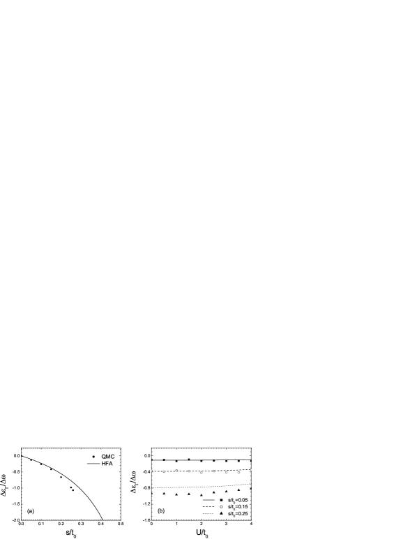
Figure 2: (a) The variation of $\Delta\epsilon_{\Gamma}/\Delta\omega$ with $s$ on a 4$\times$4 square lattice, when $U$=2.0, $\beta$=10, $\lambda_{0}$=1, $\lambda$=2. The filled circles are from QMC, and the solid curve from HFA as a guide for eyes. (b) The variations of $\Delta\epsilon_{\Gamma}/\Delta\omega$ with $U$ on a 4$\times$4 square lattice at $\beta$=10, $\lambda_{0}$=1 and $\lambda$=2. Three different values of $s$ are used to show the $s$-dependence of $\Delta\epsilon_{\Gamma}/\Delta\omega$. The discrete symbols are the results of QMC, and continuous curves by HFA as a reference.

In Fig. 2(a), we plot the ratio $\Delta\epsilon_{\Gamma}/\Delta\omega$ versus $s$, at $U$=2.0 and $\beta$=10, where $\Delta\epsilon_{\Gamma}$ is the band shift at the $\Gamma$ point of Brillouin zone [${\bf k}_{\Gamma}$=(0,0)], and $\Delta\omega$ is the isotopic change of phonon energy. The filled circles are calculated by QMC, and the solid curve by the mean-field theory with Hartree-Fork approximation (HFA) as a guide for eyes. Here both theories figure out an increase of $\Delta\epsilon_{\Gamma}/\Delta\omega$ with $s$, which means if the $e$-ph coupling is strong enough, a large band shift can be generated in the cost of a small $\Delta\omega$. In Fig. 2(b), the ratio $\Delta\epsilon_{\Gamma}/\Delta\omega$ versus $U$ are shown for three different $s$’s, where the discrete symbols and continuous curves are the QMC and HFA results, respectively. It can be seen that the ratio $\Delta\epsilon_{\Gamma}/\Delta\omega$ increases with $s$. Meanwhile, for a fixed $s$, the ratio declines slightly as $U$ increases. This behavior indicates that the band shift is owing to the $e$-ph coupling, whereas the presence of $U$ partially reduces this effect. In terms of Figs. 2(a) and 2(b), one can see the band shift is actually a measure of the $e$-ph coupling strength in the system. If the result of Ref. [2] is correct, the $e$-ph coupling must be strong in Bi2212. On the contrary, Ref. [3] shows that the coupling cannot be very large.

4 Conclusion

In summary, by using the path-integral QMC method, we study the isotopic shift in the ARPES of Bi2212 based on a model including both $e$-$e$ and off-diagonal quadratic $e$-ph interactions. Our calculation demonstrates that the band shift is primarily triggered by the $e$-ph coupling, while the presence of $e$-$e$ repulsion tends to suppress this effect.

References

References

- [1] Damascelli A, Hussain Z and Shen Z -X 2003 Rev. Mod. Phys. 75 473
- [2] Gweon G -H, Sasagawa T, Zhou S Y, Graf J, Takagi H, Lee D -H and Lanzara A 2004 Nature 430 187
- [3] Douglas J F et al. 2007 Nature 446 E5
- [4] Maksimov E G, Dolgov O V and Kulić M L 2005 Phys. Rev. B 72 212505
- [5] Martin A A and Lee M J 1995 Physica C 254 222
- [6] Tomita N and Nasu K 1997 Phys. Rev. B 56 3779
- [7] Ji K, Zheng H and Nasu K 2004 Phys. Rev. B 70 085110