Bright OB stars in the Galaxy

Abstract

Context. B-type supergiants represent an important phase in the evolution of massive stars. Reliable estimates of their stellar and wind parameters, however, are scarce, especially at mid and late spectral subtypes.

Aims. We apply the NLTE atmosphere code FASTWIND to perform a spectroscopic study of a small sample of Galactic B-supergiants from B0 to B9. By means of the resulting data and incorporating additional datasets from alternative studies, we investigate the properties of OB-supergiants and compare our findings with theoretical predictions.

Methods. Stellar and wind parameters of our sample stars are determined by line profile fitting, based on synthetic profiles, a Fourier technique to investigate the individual contributions of stellar rotation and “macro-turbulence” and an adequate approach to determine the Si abundances in parallel with micro-turbulent velocities.

Results. Due to the combined effects of line- and wind-blanketing, the temperature scale of Galactic B-supergiants needs to be revised downward, by 10 to 20%, the latter value being appropriate for stronger winds. Compared to theoretical predictions, the wind properties of OB-supergiants indicate a number of discrepancies. In fair accordance with recent results, our sample indicates a gradual decrease in $v_{\infty}$ over the bi-stability region, where the limits of this region are located at lower $T_{\rm eff}$ than those predicted. Introducing a distance-independent quantity $Q^{\prime}$ related to wind-strength, we show that this quantity is a well defined, monotonically increasing function of $T_{\rm eff}$ $outside$ this region. $Inside$ and from hot to cool, $\dot{M}$ changes by a factor (in between 0.4 and 2.5) which is much smaller than the predicted factor of 5.

Conclusions. The decrease in $v_{\infty}$ over the bi-stability region is $not$ over-compensated by an increase of $\dot{M}$ , as frequently argued, provided that wind-clumping properties on both sides of this region do not differ substantially.

1 Introduction

Hot massive stars are key objects for studying and understanding many exciting phenomena in the Universe such as re-ionisation and $\gamma$-ray bursters. Due to their powerful stellar winds hot massive stars are important contributors to the chemical and dynamical evolution of galaxies, and in the distant Universe they dominate the integrated UV radiation in young galaxies.

While the number of Galactic O and early B stars with reliably determined stellar and wind parameters has progressively increased during the last few years (e.g., Herrero et al. 2002; Repolust et al. 2004; Garcia & Bianchi 2004; Bouret et al. 2005; Martins et al. 2005; Crowther et al. 2006), mid and late B supergiants (SGs) are currently under-represented in the sample of stars investigated so far. Given the fact that B-SGs represent an important phase in the evolutionary sequence of massive stars, any study aiming to increase our knowledge of these stars would be highly valuable, since it would allow several important issues to be addressed (see below).

Compared to O-type stars the B-SG spectra are more complicated due to a larger variety of atomic species being visible, the most important among which is Silicon, the main temperature indicator in the optical domain. Thus, the reproduction of these spectra by methods of quantitative spectroscopy is a real challenge for state-of-the art model atmosphere codes, since it requires a good knowledge of the physics of these objects, combined with accurate atomic data. In turn, any discrepancy that might appear between computed and observed spectral features would help to validate the physical assumptions underlying the model calculations as well as the accuracy of the adopted atomic models and data.

Numerical simulations of the non-linear evolution of the line-driven flow instability (for a review, see Owocki 1994), with various degrees of approximation concerning the stabilising diffuse, scattered radiation field (Owocki & Puls 1996, 1999) as well as more recent simulations concentrating on the outer wind regions (Runacres & Owocki 2002, 2005), predict that hot star winds are not smooth but structured, with clumping properties depending on the distance to the stellar surface. However, recent observational studies of clumping in O-SGs have revealed inconsistencies both between results originating from different wind diagnostics, such as UV resonance lines, H_α and the IR-/radio-excess (Fullerton et al. 2006; Puls et al. 2006), and between theoretical predictions and observed constraints on the radial stratification of the clumping factor (Bouret et al. 2005; Puls et al. 2006). In addition, there are observational results which imply that clumping might depend on wind density. Because of their dense winds, B-SGs might provide additional clues to clarify these points.

Due to their high luminosities, BA-SGs can be resolved and observed, both photometrically and spectroscopically, even in rather distant, extragalactic stellar systems (e.g., Kudritzki et al. 1999; Bresolin et al. 2002; Urbaneja et al. 2003; Bianchi & Efremova 2006). This fact makes them potential standard candles, allowing us to determine distances by means of purely spectroscopic tools using the wind-momentum luminosity relationship (WLR, Kudritzki et al. 1995). Even though certain discrepancies between predicted and observed wind momenta of early B0 to B3 subtypes have been revealed (Crowther et al. 2006), relevant information about later subtypes is still missing.

During the last years, the quantitative analyses of spectra in the far-UV/UV and optical domains (e.g., Herrero et al. 2002; Bianchi & Garcia 2002; Crowther et al. 2002; Bouret et al. 2003; Repolust et al. 2004; Massey et al. 2004; Heap et al. 2006) have unambiguously shown that the inclusion of line-blocking and blanketing and wind effects (if present) significantly modifies the temperature scale of O-stars (for a recent calibration at solar metallicity, see Markova et al. 2004; Martins et al. 2005). Regarding B-SGs, particularly of later subtype, this issue has not been addressed so far, mostly due to lacking $T_{\rm eff}$ estimates.

The main goal of this study is to test and to apply the potential of our NLTE atmosphere code FASTWIND (Puls et al. 2005) to provide reliable estimates of stellar and wind parameters of SGs with temperatures ranging from 30 to 11 kK. By means of these data and incorporating additional datasets from alternative studies, we will try to resolve the questions outlined above.

In Sects. 2 and 3, we describe the stellar sample and the underlying observational material used in this study. In Sect. 4 we outline our procedure to determine the basic parameters of our targets, highlighting some problems faced during this process. In Sect. 5 the effects of line blocking/blanketing on the temperature scale of B-SGs at solar and SMC metallicities will be addressed, and in Sect. 6 we investigate the wind properties for Galactic B-SGs (augmented by O-and A-SG data), by comparison with theoretical predictions. Particular emphasis will be given to the behaviour of the mass-loss rate over the so-called bi-stability jump. Sect. 7 gives our summary and implications for future work.

Table 1: Galactic B-SGs studied in this work, together with adopted photometric data. For multiple entries, see text.

Object	spectral	member-	d	$V$	$B-V$	$(B-V)_{\rm 0}$	$M_{\rm V}$
(HD#)	type	ship
185 859	B0.5 Ia						-7.0*
190 603	B1.5 Ia+		1.57c	5.62	0.760	-0.16	-8.21
				5.62	0.54$\pm$0.02		-7.53
206 165	B2 Ib	Cep OB2	0.83a	4.76	0.246	-0.19	-6.19
198 478	B2.5 Ia	Cyg OB7	0.83a	4.81	0.571	-0.12	-6.93
				4.84	0.40$\pm$0.01		-6.37
191 243	B5 Ib	Cyg OB3	2.29a	6.12	0.117	-0.12	-6.41
			1.73b				-5.80
199 478	B8 Iae	NGC 6991	1.84d	5.68	0.408	-0.03	-7.00
212 593	B9 Iab						-6.5*
202 850	B9 Iab	Cyg OB4	1.00a	4.22	0.098	-0.03	-6.18

^a Humphreys (1978); ^b Garmany & Stencel (1992); ^c Barlow & Cohen (1977); ^d Denizman & Hack (1988)
^∗ from calibrations (Humphreys & McElroy 1984)

2 Observations and data reduction

High-quality optical spectra were collected for eight Galactic B-type SGs of spectral types B0.5 to B9 using the Coudé spectrograph of the NAO 2-m telescope of the Institute of Astronomy, Bulgarian Academy of Sciences. The observations were carried out using a BL632/14.7 grooves  mm^-1 grating in first order, together with a PHOTOMETRICS CCD (1024 x 1024, 24$\mu$) as a detector. This configuration produces spectra with a reciprocal dispersion of $\sim$0.2 Å pixel^-1 and an effective resolution of $\sim$ 2.0 pixels, resulting in a spectral resolution of $\sim$ 15 000 at H_α .

The signal-to-noise (S/N) ratio, averaged over all spectral regions referring to a given star, has typical values of 200 to 350, being lower in the blue than in the red.

We observed the wavelength range between 4 100 and 4 900 Å, where most of the strategic lines of H, He and Si ions are located, together with the region around H_α. Since our spectra sample about 200 Å, five settings were used to cover the ranges of interest. These settings are as follows:

1. From 4110 to 4310 Å (covering Si II $\lambda\lambda$4128, 4131 , Si IV $\lambda$4116 and He II $\lambda$4200).

2. From 4315 to 4515 Å (He I $\lambda\lambda$4387, 4471 and H_γ ).

3. From 4520 to 4720 Å (Si III $\lambda\lambda$4553, 4568, 4575, He I $\lambda$4713 and He II $\lambda\lambda$4541, 4686).

4. The region around H_β including Si III $\lambda\lambda$4813, 4820, 4829 and He I $\lambda$4922.

5. The region around H_α including He I $\lambda$6678 and He II $\lambda\lambda$6527, 6683.

To minimise the effects of temporal spectral variability (if any), all spectra referring to a given star were taken one after the other, with a time interval between consecutive exposures of about half an hour. Thus, we expect our results to be only sensitive to temporal variability of less than 2 hours.

The spectra were reduced following standard procedures and using the corresponding IRAF routines.

3 Sample stars

Table 1 lists our stellar sample, together with corresponding spectral and photometric characteristics, as well as association/cluster membership and distances, as adopted in the present study. For hotter and intermediate temperature stars, spectral types and luminosity classes (Column 2) were taken from the compilation by Howarth et al. (1997), while for the remainder, data from $SIMBAD$ have been used.

Since $HIPPARCOS$ based distances are no longer reliable in the distance range considered here (e.g., de Zeeuw et al. 1999; Schröder et al. 2004), we have adopted photometric distances collected from various sources in the literature (Column 4). In particular, for stars which are members of OB associations, we drew mainly from Humphreys (1978) but also consulted the lists published by Garmany & Stencel (1992) and by Barlow & Cohen (1977). In most cases, good agreement between the three datasets was found, and only for Cyg OB3 did the distance modulus provided by Humphreys turned out to be significantly larger than that provided by Garmany & Stencel. In this latter case two entries for $d$ are given in Table 1.

Apart from those stars belonging to the OB associations, there are two objects in our sample which have been recognised as cluster members: HD 190 603 and HD 199 478. The former was previously assigned as a member of Vul OB2 (e.g. Lennon et al. 1992), but this assignment has been questioned by McErlean et al. (1999) who noted that there are three aggregates at approximately 1, 2 and 4 kpc in the direction of HD 190 603. Since it is not obvious to which of them (if any) this star belongs, they adopted a somewhat arbitrary distance of 1.5 kpc. This value is very close to the estimate of 1.57 kpc derived by Barlow & Cohen (1977), and it is this latter value which we will use in the present study. However, in what follows we shall keep in mind that the distance to HD 190 603 is highly uncertain. For the second cluster member, HD 199 478, a distance modulus to its host cluster as used by Denizman & Hack (1988) was adopted.

Visual magnitudes, $V$, and $B-V$ colours (Column 5 and 6) have been taken from the HIPPARCOS Main Catalogue (I/239). While for the majority of sample stars the HIPPARCOS photometric data agree quite well (within 0.01 to 0.04 mag both in $V$ and $B-V$) with those provided by SIMBAD, for two of them (HD 190 603 and HD 198 478) significant differences between the two sets of $B-V$ values were found. In these latter cases two entries for $B-V$ are given, where the second one represents the mean value averaged over all measurements listed in SIMBAD).

Absolute magnitudes, M_V (Column 8), were calculated using the standard extinction law with $R=3.1$ combined with intrinsic colours, $(B-V)_{\rm 0}$, from Fitzpatrick & Garmany (1990) (Column 7) and distances, $V$ and $B-V$ magnitudes as described above. For the two stars which do not belong to any cluster/association (HD 185 859 and HD 212 593), absolute magnitudes according to the calibration by Humphreys & McElroy (1984) have been adopted.

For the majority of cases, the absolute magnitudes we derived, agree within $\pm$0.3 mag with those provided by the Humphreys-McElroy calibration. Thus, we adopted this value as a measure for the uncertainty in M_V for cluster members (HD 199 478) and members of spatially more concentrated OB associations (HD 198 478 in Cyg OB7, see Crowther et al. 2006). For other stars with known membership, a somewhat larger error of $\pm$0.4 mag was adopted to account for a possible spread in distance within the host association. Finally, for HD 190 603 and those two stars with calibrated M_V, we assumed a typical uncertainty of $\Delta$M_V = $\pm$0.5 mag, representative for the spread in M_V of OB stars within a given spectral type (Crowther 2004).

4 Determination of stellar and wind parameters

The analysis presented here was performed with FASTWIND, which produces spherically symmetric, NLTE, line-blanketed model atmospheres and corresponding spectra for hot stars with winds. While detailed information about the latest version used here can be found in Puls et al. (2005), we highlight only those points which are important for our analysis of B stars.

• In addition to H and He, Silicon is used as an explicit element (i.e., by means of a detailed model atom and using a comoving frame transport for the bound-bound transitions). All other elements (e.g., C, N, O, Fe, Ni etc.) are treated as background elements, where the major difference (compared to the explicit ones) relates to the line transfer, which is performed within the Sobolev approximation.

• A detailed description of the Silicon atomic model can be found in Trundle et al. (2004).

• Since previous applications of FASTWIND have concentrated on O and early B stars, we briefly note that correct treatment of cooler stars requires sufficiently well described iron group ions of stages II/III, whose lines are dominating the background opacities for these objects. Details of the corresponding model atoms and line-lists (from superstructure, Eissner et al. 1974; Nussbaumer & Storey 1978, augmented by data from Kurucz 1992) can be found in Pauldrach et al. (2001). In order to rule out important effects from still missing data, we have constructed an alternative dataset which uses all Fe/Ni II/III lines from the Kurucz line-list. Corresponding models (in particular temperature structure and emergent fluxes) turned out to remain almost unaffected by this alteration, so we are confident that our original database is fairly complete, and can be used for calculations roughly down to 10 kK.

• A consistent temperature stratification utilising a flux-correction method in the lower wind and the thermal balance of electrons in the outer part is calculated, with a transition point between the two approaches located roughly at a Rossland optical depth of $\tau_{\rm R}\approx 0.5$ (in dependence of wind density).

To allow for an initial assessment of the basic parameters, a coarse grid of models was generated using this code (appropriate for the considered targets). The grid involves 270 models covering the temperature range between 12 and 30 kK (with increments of 2 kK) and including $\log g$ values from 1.6 to 3.4 (with increments of 0.2 dex). An extended range of wind-densities, as combined in the optical depth invariant $Q$ (=$\dot{M}$ /($v_{\infty}$ $R_{\star}$ )^1.5, cf. Puls et al. 1996) has been accounted for as well, to allow for both thin and thick winds.

All models have been calculated assuming solar Helium ($Y_{\rm He}$ = 0.10, with $Y_{\rm He}=N({\rm He})/N({\rm H})$) and Silicon abundance (log (Si/H) = -4.45 by number, cf. Grevesse & Sauval 1998 and references therein), and a micro-turbulent velocity, $v_{\rm mic}$ , of 15 km s^-1 for hotter and 10 km s^-1 for cooler subtypes, with a border line at 20 kK.

By means of this model grid, initial estimates on $T_{\rm eff}$ , $\log g$ and $\dot{M}$ were obtained for each sample star. These estimates were subsequently used to construct a smaller subgrid, specific for each target, to derive the final, more exact values of the stellar and wind parameters (including Y_He, log (Si/H) and $v_{\rm mic}$ ).

Radial velocities

To compare observed with synthetic profiles, radial velocities and rotational speeds of all targets have to be known. We started our analysis with radial velocities taken from the General Catalogue of Mean Radial Velocities (III/213, Barbier-Brossat & Figon 2000). These values were then modified to obtain better fits to the analysed absorption profiles. In doing so we gave preference to Silicon rather than to Helium or Hydrogen lines since the latter might be influenced by (asymmetrical) wind absorption/emission. The finally adopted $V_{\rm r}$ -values which provide the “best” fit to most of the Silicon lines are listed in Column 3 of Table 2. The accuracy of these estimates is typically $\pm$ 2km s^-1 .

Table 2: Radial velocities (from Si), projected rotational velocities, macro- and micro-turbulent velocities (all in km s^-1 ) and Si abundances, given as log [$N$(Si)/$N$(H] + 12, of the sample stars as determined in the present study. The number in brackets refers to the number of lines used to derive $v\sin i$ and $v_{\rm mac}$ .

Object	Sp	$V_{\rm r}$	$v\sin i$	$v_{\rm mac}$	$v_{\rm mic}$	Si abnd
HD 185 859	B0.5 Ia	12	62(5)	58(3)	18	7.51
HD 190 603	B1.5 Ia+	50	47(8)	60(3)	15	7.46
HD 206 165	B2 Ib	0	45(7)	57(3)	8	7.58
HD 198 478	B2.5 Ia	8	39(9)	53(3)	8	7.58
HD 191 243	B5 Ib	25	38(4)	37(3)	8	7.48
HD 199 478	B8 Iae	-12	41(4)	40(3)	8	7.55
HD 212 593	B9 Iab	-13	28(3)	25(3)	7	7.65
HD 202 850	B9 Iab	13	33(3)	33(3)	7	7.99

4.1 Projected rotational velocities and macro-turbulence

As a first guess for the projected rotational velocities of the sample stars, $v\sin i$ , we used values obtained by means of the Spectral type - $v\sin i$  calibration for Galactic B-type SGs provided by Abt et al. (2002). However, during the fitting procedure it was found that (i) these values provide poor agreement between observed and synthetic profiles and (ii) an additional line-broadening agent must be introduced to improve the quality of the fits. These findings are consistent with similar results from earlier investigations claiming that absorption line spectra of O-type stars and B-type SGs exhibit a significant amount of broadening in excess to the rotational broadening (Rosenhald 1970; Conti & Ebbets 1977; Lennon et al. 1993; Howarth et al. 1997). Furthermore, although the physical mechanism responsible for this additional line-broadening is still not understood we shall follow Ryans et al. (2002) and refer to it as “macro-turbulence”.

Figure 1: Projected rotational (left panel) and macro-turbulent (right panel) velocities of OB-SGs (spectral types refer to O-stars, i.e., 10 corresponds to B0 and 20 to A0). Data derived in the present study are marked with diamonds while crosses refer to published data (Dufton et al. 2006; Simon-Diaz & Herrero 2007).

Since the effects of macro-turbulence are similar to those caused by axial rotation, (i.e., they do not change the line strengths but “only” modify the profile shapes) and since stellar rotation is a key parameter, such as for stellar evolution calculation (e.g., Meynet & Maeder 2000, Hirschi et al. 2005 and references therein), it is particularly important to distinguish between the individual contributions of these two processes.

There are at least two possibilities to approach this problem: either exploiting the goodness of the fit between observed and synthetic profiles (Ryans et al. 2002) or analysing the shape of the Fourier transforms (FT) of absorption lines (Gray 1973, 1975; Simon-Diaz & Herrero 2007). Since the second method has been proven to provide better constraints (Dufton et al. 2006), we followed this approach to separate and measure the relative magnitudes of rotation and macro-turbulence.

The principal idea of the FT method relates to the fact that in Fourier space the convolutions of the ”intrinsic line profile” (which includes the natural, thermal, collisional/Stark and microturbulence broadening) with the instrumental, rotational and macro-turbulent profiles, become simple products of the corresponding Fourier components, thus allowing the contributions of the latter two processes to be separated by simply dividing the Fourier components of the observed profile by the components of the thermal and instrumental profile.

The first minimum of the Fourier amplitudes of the obtained residual transform will then fix the value of $v\sin i$  while the shape of the first side-lobe of the same transform will constrain $v_{\rm mac}$.

The major requirements to obtain reliable results from this method is the presence of high quality spectra (high S/N ratio and high spectral resolution) and to analyse only those lines which are free from strong pressure broadening but are still strong enough to allow for reliable $v\sin i$  estimates.

For the purpose of the present analysis, we have used the implementation of the FT technique as developed by Simon-Diaz & Herrero (2007) (based on the original method proposed by Gray 1973, 1975) and applied it to a number of preselected absorption lines fulfilling the above requirements. In particular, for our sample of early B subtypes, the Si III multiplet around 4553 Å but also lines of O II and N II were selected, whereas for the rest the Si II doublet around 4130 Å and the Mg II line at $\lambda$4481 were used instead.

The obtained pairs of ($v\sin i$ , $v_{\rm mac}$ ), averaged over the measured lines, were then used as input parameters for the fitting procedure and subsequently modified to improve the fits. The finally adopted values of $v\sin i$  and $v_{\rm mac}$  are listed in Columns 4 and 5 of Table 2, respectively. Numbers in brackets refer to the number of lines used for this analysis. The uncertainty of these estimates is typically less than $\pm$10 km s^-1, being largest for those stars with a relatively low rotational speed, due to the limitations given by the resolution of our spectra ($\sim$35 km s^-1 ). Although the sample size is small, the $v\sin i$  and $v_{\rm mac}$  data listed in Table 2 indicate that:

$\bullet$ in none of the sample stars is rotation alone able to reproduce the observed line profiles (width and shape).

$\bullet$ both $v\sin i$  and $v_{\rm mac}$  decrease towards later subtypes (lower $T_{\rm eff}$ ), being about a factor of two lower at B9 than at B0.5.

$\bullet$ independent of spectral subtype, the size of the macro-turbulent velocity is similar to the size of the projected rotational velocity.

$\bullet$ also in all cases, $v_{\rm mac}$  is well beyond the speed of sound.

Compared to similar data from other investigations for stars in common (e.g. Rosenhald 1970; Howarth et al. 1997), our $v\sin i$  estimates are always smaller, by up to 40%, which is understandable since these earlier estimates refer to an interpretation in terms of rotational broadening alone.

On the other hand, and within a given spectral subtype, our estimates of $v\sin i$  and $v_{\rm mac}$  are consistent with those derived by Dufton et al. (2006) and Simon-Diaz & Herrero (2007) (see Figure 1). From these data it is obvious that both $v\sin i$  and $v_{\rm mac}$ appear to decrease (almost monotonically) in concert, when proceeding from early-O to late B-types.

4.2 Effective temperatures, $T_{\rm eff}$ 

For B-type stars the primary temperature diagnostic at optical wavelengths is Silicon (Becker & Butler 1990; Kilian et al. 1991; McErlean et al. 1999; Trundle et al. 2004) which shows strong lines from three ionisation stages through all the spectral types: Si III/Si IV for earlier and Si II/Si III for later subtypes, with a “short” overlap at B1.5 - B2. To evaluate $T_{\rm eff}$ (and $\log g$ ), to a large extent we employed the method of line profile fitting instead of using fit diagrams (based on EWs), since in the latter case the corresponding estimates rely on interpolations and furthermore do not account for the profile shape. Note, however, that for certain tasks (namely the derivation of the Si-abundance together with the micro-turbulent velocity), EW-methods have been applied (see below).

In particular, to determine $T_{\rm eff}$ we used the Si II features at $\lambda\lambda$4129, 4131, the Si III features at $\lambda\lambda$4553, 4568, 4575 and at $\lambda\lambda$4813, 4819, 4828, with a preference on the first triplet (see

Figure 2: Effects of micro-turbulence on the strength of Si IV 4116/Si III 4553 (left panel) and Si II 4128/Si III 4553 (right panel) equivalent width ratios for B-type SGs. $V_{\rm mic}$ ranging from 4 to 18 km s^-1 , with increments of 4 km s^-1 . Triangles refer to the lowest value of $v_{\rm mic}$, squares to the highest (see text).

below) and the Si IV feature at $\lambda$4116. In addition, for stars of spectral type B2 and earlier the Helium ionisation balance was exploited as an additional check on $T_{\rm eff}$ , involving He I transitions at $\lambda\lambda$4471, 4713, 4387, 4922 and He II transitions at $\lambda\lambda$4200, 4541, 4686.

4.2.1 Micro-turbulent velocities and Si abundances

Though the introduction of a non-vanishing micro-turbulent velocity can significantly improve the agreement between synthetical profiles and observations (McErlean et al. 1998; Smith & Howarth 1998), it is still not completely clear whether such a mechanism (operating on scales below the photon mean free path) is really present or whether it is an artefact of some deficiency in the present-day description of model atmospheres (e.g., McErlean et al. 1998; Villamariz & Herrero 2000 and references therein).

Since micro-turbulence can strongly affect the strength of Helium and metal lines, its inclusion into atmospheric models and profile functions can significantly modify the derived stellar abundances but also effective temperatures and surface gravities (the latter two parameters mostly indirectly via its influence on line blanketing: stronger $v_{\rm mic}$ implies more blocking/back-scattering, and thus lower $T_{\rm eff}$ .)

Whereas Villamariz & Herrero (2000) showed the effects of $v_{\rm mic}$ to be relatively small for O-type stars, for B-type stars this issue has only been investigated for early B1-B2 giants (e.g., Vrancken et al. 2000) and a few, specific BA supergiants (e.g. Urbaneja 2004; Przybilla et al. 2006). Here, we report on the influence of micro-turbulence on the derived effective temperatures for the complete range of B-type SGs. For this purpose we used a corresponding sub-grid of FASTWIND models with $v_{\rm mic}$ ranging from 4 to 18 km s^-1 (with increments of 4 km s^-1 ) and $\log Q$ values corresponding to the case of relatively weak winds. Based on these models we studied the behaviour of the SiIV4116/SiIII4553 and SiII4128/SiIII4553 line ratios and found these ratios to be almost insensitive to variations in $v_{\rm mic}$ (Fig. 2), except for the case of SiII/SiIII beyond 18 kK where differences of about 0.3 to 0.4 dex can be seen (and are to be expected, due to the large difference in absolute line-strengths caused by strongly different ionisation fractions). Within the temperature ranges of interest (18 $\leq$ $T_{\rm eff}$  $\leq$ 28 kK for SiIV/SiIII and 12 $\leq$ $T_{\rm eff}$  $\leq$ 18 kK for SiII/SiIII), however, the differences are relatively small, about 0.15 dex or less, resulting in temperature differences lower than 1 000 K, i.e., within the limits of the adopted uncertainties (see below).

Based on these results, we relied on the following strategy to determine $T_{\rm eff}$, $v_{\rm mic}$  and Si abundances. As a first step, we used the FASTWIND model grid as described previously (with $v_{\rm mic}$ =10 and 15 km s^-1 and “solar” Si abundance) to put initial constraints on the stellar and wind parameters of the sample stars. Then, by varying $T_{\rm eff}$  (but also $\log g$ , $\dot{M}$  and velocity-field parameter $\beta$) within the derived limits and by changing $v_{\rm mic}$ within $\pm$5 km s^-1 to obtain a satisfactory fit to most of the strategic Silicon lines, we fixed $T_{\rm eff}$ /$\log g$ and derived rough estimates of $v_{\rm mic}$. Si abundances and final values for $v_{\rm mic}$ resulted from the following procedure: for each sample star a grid of 20 FASTWIND models was calculated, combining four abundances and five values of micro-turbulence (ranging from 10 to 20 km s^-1 or from 4 to 12 km s^-1, to cover hot and cool stars, respectively). By means of this grid, we determined those abundance ranges which reproduce the observed individual EWs (within the corresponding errors) of several previously selected Si lines from different ionisation stages. Subsequently, we sorted out the value of $v_{\rm mic}$ which provides the best overlap between these ranges,

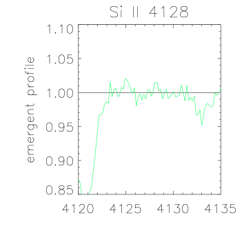
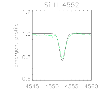
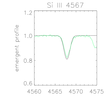
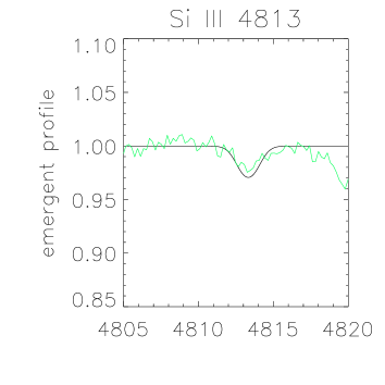
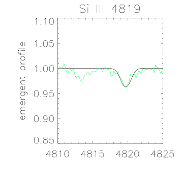
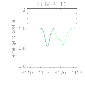
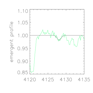
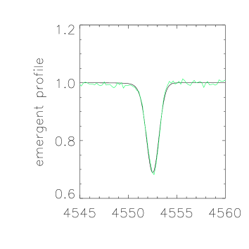
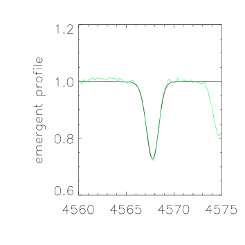
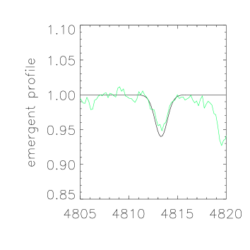
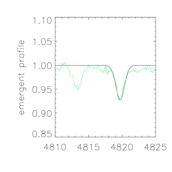
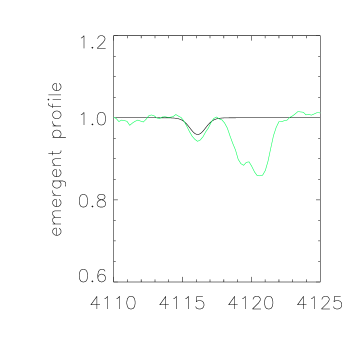
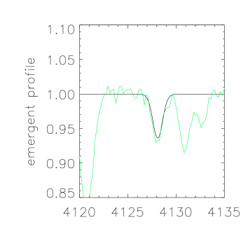
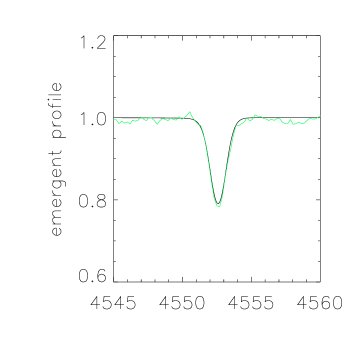
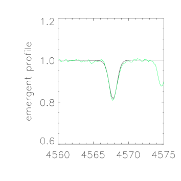
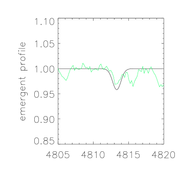
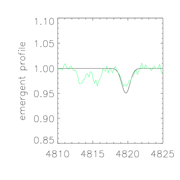
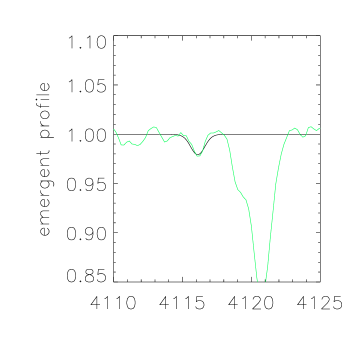
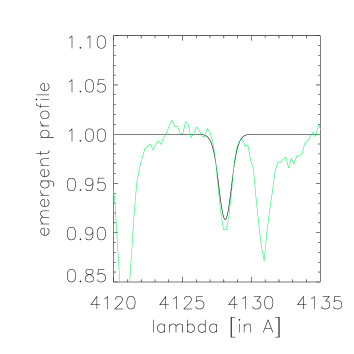
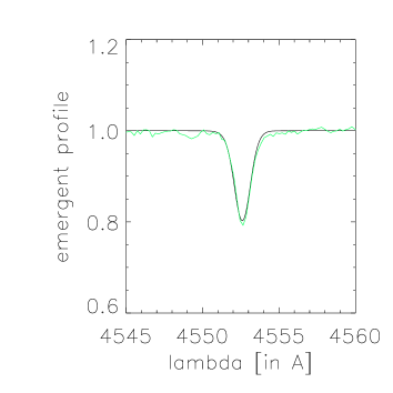
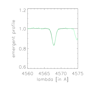
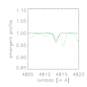
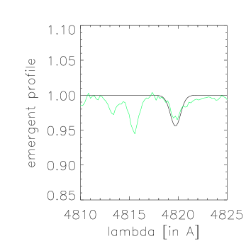
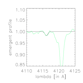
Figure 3: Examples for the quality of our final (“best”) Silicon line-profile fits. From top to bottom: HD 185 859 (B0.5Ia), HD 190 603 (B1.5Ia+), HD 206 165 (B2Ib) and HD 198 478 (B2.5Ia). Note the systematic discrepancy between synthetic and observed profiles of the Si III lines at $\lambda\lambda$4813,4819.

i.e., defines a unique abundance together with appropriate errors (for more details, see e.g. Urbaneja 2004; Simon-Diaz et al. 2006 and references therein).

Our final results for $v_{\rm mic}$ were almost identical (within about $\pm$1 km s^-1 ) to those derived from the “best” fit to Silicon. Similarly, for all but one star, our final estimates for the Si abundance are quite similar to the initially adopted “solar” one, within $\leq\pm$0.1 dex, and only for HD 202 850 an increase of 0.44 dex was found. Given that Si is not involved in CNO nuclear processing, the latter result is difficult to interpret. On the one hand, fitting/analysis problems are highly improbable, since no unusual results have been obtained for the other late B-SG, HD 212 593. Indeed, the overabundance is almost “visible” because the EWs of at least 2 of the 3 strategic Si lines are significantly larger (by about 20 to 40%) in HD 202 850 than in HD 212 593. On the other hand, the possibility that this star is metal rich seems unlikely given its close proximity to our Sun. Another possibility might be that HD 202 850 is a Si star, though its magnetic field does not seem particularly strong (but exceptions are still known, e.g. V 828 Her B9sp, EE Dra B9, Bychkov et al. 2003). A detailed abundance analysis may help to solve this puzzling feature.

Finally, we have verified that our newly derived Si abundances (plus $v_{\rm mic}$ -values) do not affect the stellar parameters (which refer to the initial abundances), by means of corresponding FASTWIND models. Though an increase of 0.44 dex (the exceptional case of HD 202 850) makes the Si-lines stronger, this strengthening does not affect the derived $T_{\rm eff}$, since the latter parameter depends on line ratios from different ionisation stages, being thus almost independent of abundance. In each case, however, the quality of the Silicon line-profile fits has been improved, as expected.

In Column 6 and 7 of Table 2 we present our final values for $v_{\rm mic}$  and Si abundance. The error of these estimates depends on the accuracy of the measured equivalent widths (about 10%) and is typically about $\pm$2 km s^-1 and $\pm$0.15 dex for $v_{\rm mic}$  and the logarithmic Si abundance, respectively. A closer inspection of these data indicates that the micro-turbulent velocities of B-type SGs might be closely related to spectral type (see also McErlean et al. 1999), being highest at earlier (18 km s^-1 at B0.5) and lowest at later B subtypes (7 km s^-1 at B9). Interestingly, the latter value is just a bit larger than the typical values reported for A-SGs (3 to 8 km s^-1 , e.g., Venn 1995), thus implying a possible decline in micro-turbulence towards even later spectral types.

4.2.2 Silicon line profiles fits – a closer inspection

During our fitting procedure, we encountered the problem that the strength of the Si III multiplet near 4813 Å was systematically over-predicted (see Fig. 3 for some illustrative examples). Though this discrepancy is not very large (and vanishes if $T_{\rm eff}$ is modified within ($\pm$500 K), this discrepancy might point to some weaknesses in our model assumptions or data. Significant difficulties in reproducing the strength of Si III multiplets near 4553 and 4813 Å have also been encountered by McErlean et al. (1999) and by Becker & Butler (1990). While in the former study both multiplets were found to be weaker in their lowest-gravity models with $T_{\rm eff}$  beyond 22 500 K, in the latter study the second multiplet was overpredicted, by a factor of about two.

The most plausible explanation for the problems encountered by McErlean et al. (1999) (which are opposite to ours) is the neglect of line-blocking/blanketing and wind effects in their NLTE model calculations, as already suggested by the authors themselves. The discrepancies reported by Becker & Butler (1990), on the other hand, are in qualitative agreement to our findings, but much more pronounced (a factor of two against 20 to 30%). Since both studies use the same Si III model ion whilst we have updated the oscillator strengths of the multiplet near 4553 Å(!) drawing from the available atomic databases, we suggest that it is these improved oscillator strengths in conjunction with modern stellar atmospheres which have reduced the noted discrepancy.

Regardless of these improvements, the remaining discrepancy must have an origin, and there are at least two possible explanations: (i) too small an atomic model for Si III (cutoff effects) and/or (ii) radially stratified micro-turbulent velocities (erroneous oscillator strengths cannot be excluded, but are unlikely, since all atomic databases give similar values).

The first possibility was discussed by Becker & Butler (1990) who concluded that this defect cannot be the sole origin of their problem, since the required corrections are too large and furthermore would affect the other term populations in an adverse manner. Because the discrepancy found by us has significantly decreased since then, the possibility of too small an atomic model can no longer be ruled out though. Future work on improving the complete Si atom will clarify this question.

In our analyses, we have used the same value of $v_{\rm mic}$  for all lines in a given spectrum, i.e., assumed that this quantity does not follow any kind of stratification throughout the atmosphere, whilst the opposite might actually be true (e.g. McErlean et al. 1999; Vrancken et al. 2000; Trundle et al. 2002, 2004; Hunter et al. 2006). If so, a micro-turbulent velocity being a factor of two lower than inferred from the “best” fit to Si III 4553 and the Si II doublet would be needed to reconcile calculated and observed strengths of the 4813 Å multiplet. Such a number does not seem unlikely, given the difference in line strengths, but clearly further investigations are necessary (after improving upon the atomic model) to clarify this possibility (see also Hunter et al. 2006 and references therein).

Considering the findings from above, we decided to follow Becker & Butler (1990) and to give preference to the Si III multiplet near 4553 Å throughout our analysis. Since this multiplet is observable over the whole B star temperature range while the other (4813 Å) disappears at mid-B subtypes, such a choice has the additional advantage of providing consistent results for the complete sample, from B0 to B9.

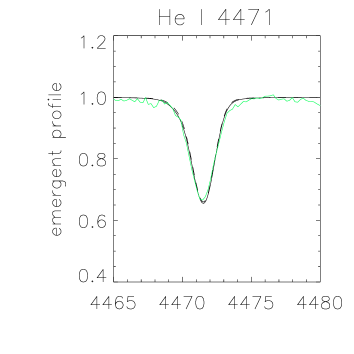
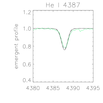
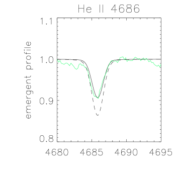
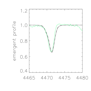
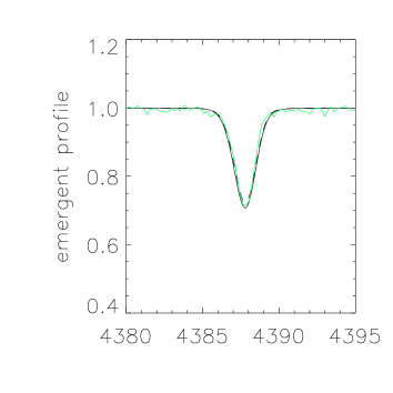
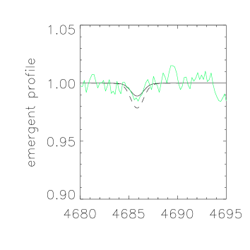
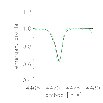
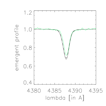
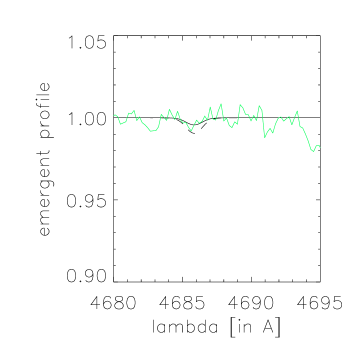
Figure 4: Observed and synthetic Helium line-profiles, calculated at the upper ($T_{\rm eff}$ + $\Delta$$T_{\rm eff}$ : dashed) and lower ($T_{\rm eff}$ - $\Delta$$T_{\rm eff}$ : solid) limit of the corresponding $T_{\rm eff}$ determined from the “best” fits to strategic Silicon lines. From top to bottom: HD 185 859 (B0.5Ia), HD 190 603 (B1.5Ia+) and HD 206 165 (B2Ib).

4.2.3 Helium line-profiles fits and Helium abundance

As pointed out in the beginning of this section, for early-B subtypes, the Helium ionisation balance can be used to determine $T_{\rm eff}$. Consequently, for the three hottest stars in our sample we used He I and He II lines to derive independent constraints on $T_{\rm eff}$, assuming helium abundances as discussed below. Interestingly, in all these cases satisfactory fits to the available strategic Helium lines could be obtained in parallel with Si IV and Si III (within the adopted uncertainties, $\Delta$$T_{\rm eff}$ =$\pm$500K). This result is illustrated in Fig. 4, where a comparison between observed and synthetic Helium profiles is shown, the latter being calculated at the upper and lower limit of the $T_{\rm eff}$ range derived from the Silicon ionisation balance. Our finding contrasts Urbaneja (2004) who reported differences in the stellar parameters beyond the typical uncertainties, if either Silicon or Helium was used independently.

Whereas no obvious discrepancy between He I singlets and triplets (“He I singlet problem”, Najarro et al. 2006 and references therein) has been seen in stars of type B1.5 and earlier, we faced several problems when trying to fit Helium in parallel with Silicon in stars of mid and late subtypes (B2 and later).

In particular, and at “normal” helium abundance ($Y_{\rm He}$ =0.1$\pm$0.02), the singlet line at $\lambda$4387 is somewhat over-predicted for all stars in this subgroup, except for the coolest one - HD 202 850. At the same time, the triplet transitions at $\lambda\lambda$4471 and 4713 have been under-predicted (HD 206 165, B2 and HD 198 478, B2.5), well reproduced (HD 191 243, B5 and HD 199 478, B8) or over-predicted (HD 212 593, B9). Additionally, in half of these stars (HD 206 165, HD 198 478, and HD 199 478) the strength of the forbidden component of He I 4471 was over-predicted, whereas in the other half this component was well reproduced. In all cases, however, these discrepancies were not so large as to prevent a globally satisfactory fit to the available He I lines in parallel with Silicon. Examples illustrating these facts are shown in Fig. 5. Again, there are at least two principle possibilities to solve these problems: to adapt the He abundance or/and to use different values of $v_{\rm mic}$ , on the assumption that this parameter varies as a function of atmospheric height (cf. Sect. 4.2.2).

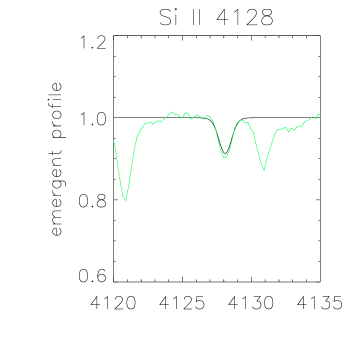
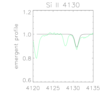
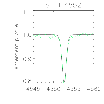
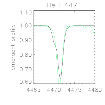
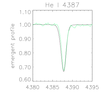
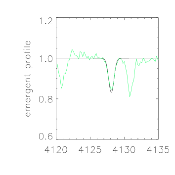
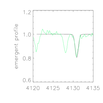
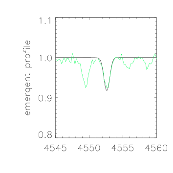
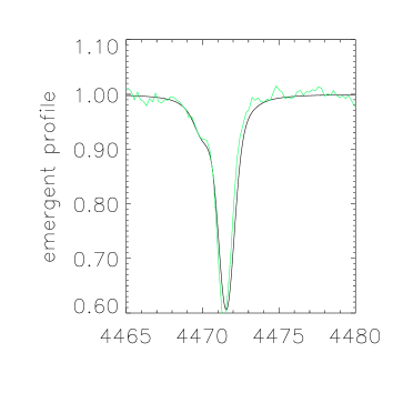
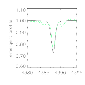
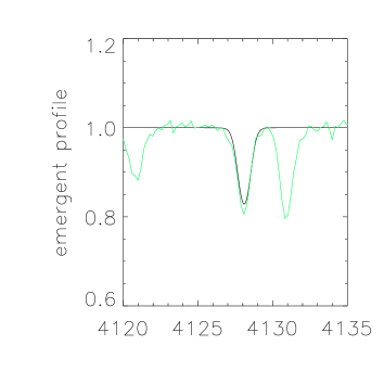
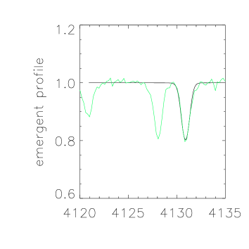
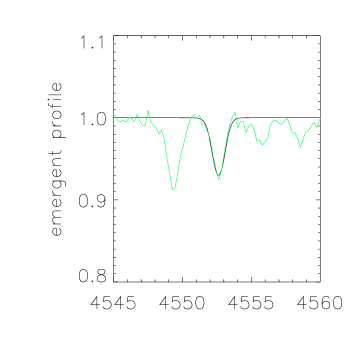
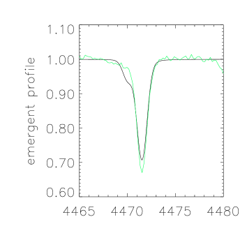
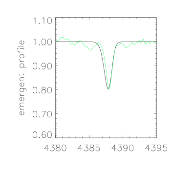
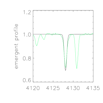
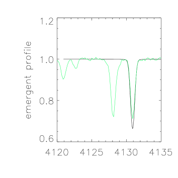
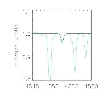
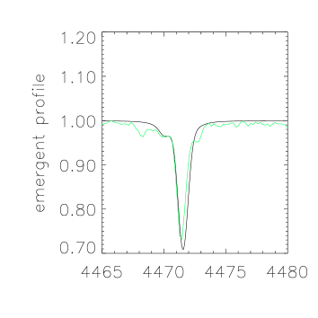
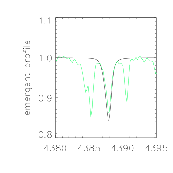
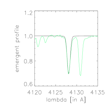
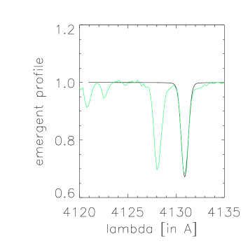
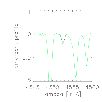
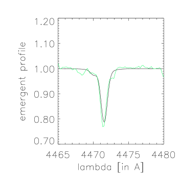
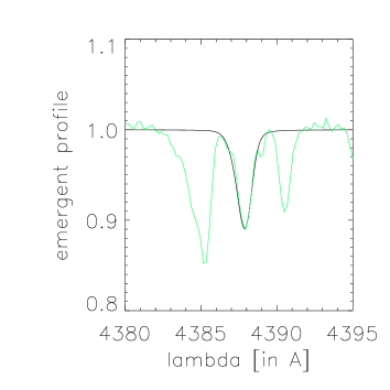
Figure 5: Final (“best”) fits to Silicon and Helium lines. From top to bottom: HD 198 478 (B2.5), HD 191 243 (B5Ib), HD 199 478 (B8ae), HD 212 593 (B9 Iab) and HD 202 850 (B9 Iab). Note that the forbidden component in the blue wing of He I $\lambda$4471 is over-predicted in a number of cases, and that the synthetic He I singlet at $\lambda$4387 is systematically too strong.

Helium abundance.

For all sample stars a “normal” helium abundance, $Y_{\rm He}$ = 0.10, was adopted as a first guess. Subsequently, this value has been adjusted (if necessary) to improve the Helium line fits. For the two hottest stars with well reproduced Helium lines (and two ionisation stages being present!), an error of only $\pm$0.02 seems to be appropriate because of the excellent fit quality. Among those, an overabundance in Helium ($Y_{\rm He}$ = 0.2) was found for the hypergiant HD 190 603, which might also be expected according to its evolutionary stage.

In mid and late B-type stars, on the other hand, the determination of $Y_{\rm He}$ was more complicated, due to problems discussed above. Particularly for stars where the discrepancies between synthetic and observed triplet and singlet lines were opposite to each other, no unique solution could be obtained by varying the Helium abundance, and we had to increase the corresponding error bars (HD 206 165 and HD 198 478). For HD 212 593, on the other hand (where all available singlet and triplet lines turned out to be over-predicted), a Helium depletion by 30 to 40% would be required to reconcile theory with observations.

All derived values are summarised in Column 8 of Table 3, but note that alternative fits of similar quality are possible for those cases where an overabundance/depletion in He has been indicated, namely by using a solar Helium content and $v_{\rm mic}$  being a factor of two larger/lower than inferred from Silicon: Due to the well known dichotomy between abundance and micro-turbulence (if only one ionisation stage is present), a unique solution is simply not possible, accounting for the capacity of the diagnostic tools used here.

Column 4 of Table 3 lists all effective temperatures as derived in the present study. As we have seen, these estimates are influenced by several processes and estimates of other quantities, among which are micro- and macro-turbulence, He and Si abundances, surface gravity and mass-loss rate (where the latter two quantities are discussed in the following). Nevertheless, we are quite confident that, to a large extent, we have consistently and partly independently (regarding $v_{\rm mic}$ , $v_{\rm mac}$ and Si abundances) accounted for these influences. Thus, the errors in our $T_{\rm eff}$ estimates should be dominated by uncertainties in the fitting procedure, amounting to about $\pm$500 K. Of course, these are differential errors assuming that physics complies with all our assumptions, data and approximations used within our atmosphere code.

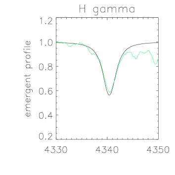
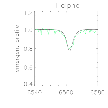
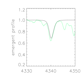
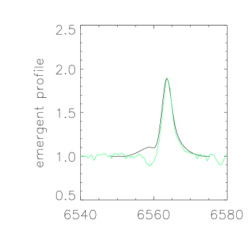
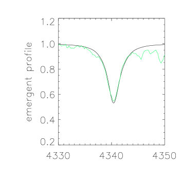
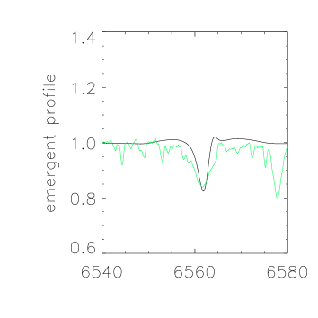
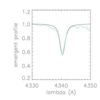
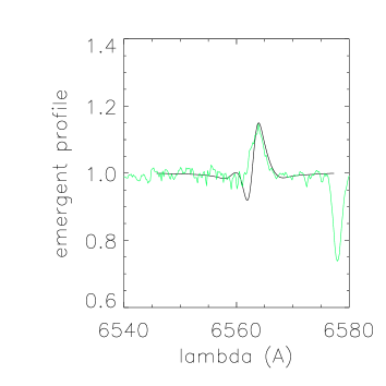
Figure 6: Fit quality for H_γ and H_α, for early and mid subtypes. From top to bottom: HD 185 859 (B0.5Ia), HD 190 603 (B1.5Ia+), HD 206 165 (B2Ib) and HD 198 478 (B2.5).

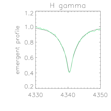
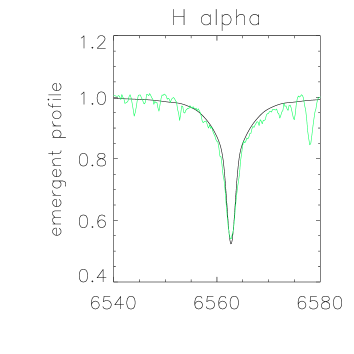
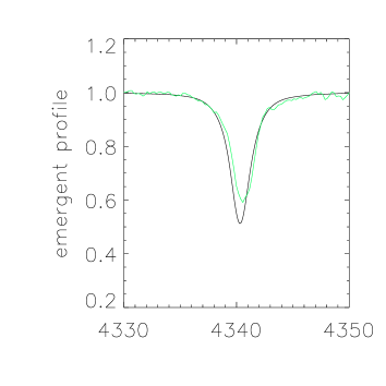
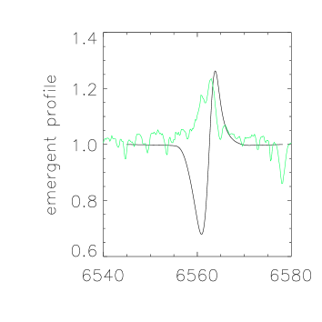
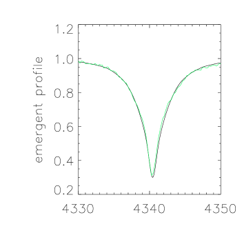
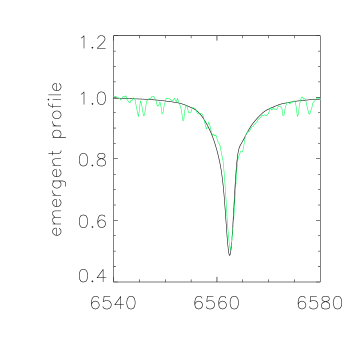
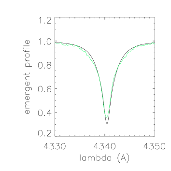
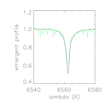
Figure 7: As for Fig. 6, but for late B subtypes. From top to bottom: HD 191 243 (B5Ib), HD 199 478 (B8ae), HD 212 593 (B9Iab) and HD 202 850 (B9Iab).

4.3 Surface gravity

Classically, the Balmer lines wings are used to determine the surface gravity, $\log g$, where only higher members (H_γ and H_δ when available) have been considered in the present investigation to prevent a bias because of potential wind-emission effects in H_α and H_β . Note that due to stellar rotation the $\log g$  values derived from such diagnostics are only $effective$ values. To derive the true gravities, $\log g_{\rm true}$, required to calculate masses, one has to apply a centrifugal correction (approximated by $v\sin i$ ²/$R_{\star}$ ), though for all our sample stars this correction was found to be typically less than 0.03 dex.

Corresponding values for effective and corrected surface gravities are listed in Columns 5 and 6 of Table 3. The error of these estimates was consistently adopted as $\pm$ 0.1 dex due to the rather good quality of the fits and spectra (because of the small centrifugal correction, corresponding errors can be neglected) except for HD 190 603 and HD 199 478 where an error of $\pm$0.15 dex was derived instead. This point is illustrated in Figs 6 and 7 where our final (“best”) fits to the observed H_γ profiles are shown. Note that the relatively large discrepancies in the cores of HD 190 603 and HD 199 478 might be a result of additional emission/absorption from large-scale structures in their winds (Rivinius et al. 1997; Markova et al. 2007), which cannot be reproduced by our models (see also Sec. 4.5 below). At least for HD 190 603, an alternative explanation in terms of too large a mass-loss rate (clumping effects in H_α ) is possible as well.

4.4 Stellar radii, luminosities and masses

The input radii used to calculate our model grid have been drawn from evolutionary models. Of course, these radii are somewhat different from the finally adopted ones (listed in Column 7 of Table 3) which have been derived following the procedure introduced by Kudritzki (1980) (using the de-reddened absolute magnitudes from Table 1 and the theoretical fluxes of our models). With typical uncertainties of $\pm$500 K in our $T_{\rm eff}$ and of $\pm$0.3 to 0.5 mag in M_V , the error in the stellar radius is dominated by the uncertainty in M_V , and is of the order of $\Delta$log $R_{\star}$ = $\pm$0.06…0.10, i.e., less than 26% in $R_{\star}$.

Luminosities have been calculated from the estimated effective temperatures and stellar radii, while masses were inferred from the “true” surface gravities. These estimates are given in Columns 9 and 10 of Table 3, respectively. The corresponding errors are less then $\pm$0.21 dex in $\log L/L_{\odot}$ and $\pm$0.16 to 0.25 dex in log $M_{\star}$ .

The spectroscopically estimated masses of our SG targets range from 7 to 53 $M_{\odot}$ . Compared to the evolutionary masses from Meynet & Maeder (2000) and apart from two cases, our estimates are generally lower, by approximately 0.05 to 0.38 dex, with larger differences for less luminous stars. While for some stars the discrepancies are less than or comparable to the corresponding errors (e.g., HD 185 859, HD 190 603 first entry, HD206 165), they are significant for some others (mainly at lower luminosities) and might indicate a “mass discrepancy”, in common with previous findings (Crowther et al. 2006; Trundle et al. 2005).

4.5 Wind parameters

Terminal velocities.

For the four hotter stars in our sample, individual terminal velocities are available in the literature, determined from UV P Cygni profiles (Lamers et al. 1995; Prinja et al. 1990; Howarth et al. 1997). For these stars, we adopted the estimates from Howarth et al. (1997). Interestingly, the initially adopted value of 470 km s^-1 for $v_{\infty}$ of HD 198 478 did not provide a satisfactory fit to H_α, which in turn required a value of about 200 km s^-1. This is at the lower limit of the “allowed” range, since the photospheric escape velocity, $v_{\rm esc}$, is of the same order. Further investigations, however, showed that at a different observational epoch the H_α profile of HD 198 478 indeed has extended to about 470 km s^-1 (Crowther et al. 2006). Thus, for this object we considered a rather large uncertainty, accounting for possible variations in $v_{\infty}$.

Regarding the four cooler stars, on the other hand, we were forced to estimate $v_{\infty}$ by employing the spectral type - terminal velocity calibration provided by Kudritzki & Puls (2000), since no literature values could be found and since archival data do not show saturated P Cygni profiles which could be used to determine $v_{\infty}$ . In all but one of these objects (HD 191 243, first entry), the calibrated $v_{\infty}$ -values were lower than the corresponding escape velocities, and we adopted $v_{\infty}$ = $v_{\rm esc}$ to avoid this problem.

The set of $v_{\infty}$ -values used in the present study is listed in Column 11 of Table 3. The error of these data is typically less than 100 km s^-1 (Prinja et al. 1990) except for the last four objects where an asymmetric error of -25/+50% was assumed instead, allowing for a rather large insecurity towards higher values.

Velocity exponent $\beta$.

In stars with denser winds (H_α in emission) $\beta$ can be derived from H_α with relatively high precision and in parallel with the mass loss rate, due to the strong sensitivity of the H_α profile shape on this parameter (but see below). On the other hand, for stars with thin winds (H_α in absorption) the determination of $\beta$ from optical spectroscopy alone is (almost) impossible and a typical value of $\beta=1$ was consistently adopted, but lower and larger values have been additionally used to constrain the errors. Note that for two of these stars we actually found indications for values larger than $\beta$=1.0 (explicitly stated in Table 3).

Mass-loss rates,

$\dot{M}$, have been derived from fitting the observed H_α profiles with model calculations. The obtained estimates are listed in column 13 of Table 3. Corresponding errors, accumulated from the uncertainties in $Q$, $R_{\star}$ and $v_{\infty}$ , are typically less than $\pm$0.16 dex for the three hotter stars in our sample and less than $\pm$0.26 dex for the rest, due to more insecure values of $v_{\infty}$ and $Q$.

Table 3: Final results for our sample of Galactic B-SGs: Stellar and wind parameters adopted ($\rightarrow$M_V ) and derived using FASTWIND. $T_{\rm eff}$ in kK, $R_{\star}$ in $R_{\odot}$ , $M_{\star}$ in $M_{\odot}$ , $v_{\infty}$ in km s^-1 , $\dot{M}$ in $10^{-6}{\rm M_{\odot}/yr}$. $D_{\rm mom}$ (in cgs-units) denotes the modified wind-momentum rate. High precision $\beta$-values are given bold-faced. For non-tabulated errors, see text.

Object	Sp	MV	$T_{\rm eff}$	$\log g$	$\log g_{\rm true}$	$R_{\star}$	$Y_{\rm He}$	$\log L/L_{\odot}$	$M_{\star}$	$v_{\infty}$	$\beta$	log $\dot{M}$	$\log D_{\rm mom}$
HD 185 859	B0.5 Ia	-7.00	26.3	2.95	2.96	35	0.10$\pm$0.02	5.72	41${}^{\rm+27}_{\rm-16}$	1 830	1.1$\pm$0.1a)	-5.82$\pm$0.13	29.01$\pm$0.20
HD 190 603	B1.5 Ia+	-8.21	19.5	2.35	2.36	80	0.20$\pm$0.02	5.92	53${}^{\rm+41}_{\rm-23}$	485	2.9$\pm$0.2	-5.70$\pm$0.16	28.73$\pm$0.22
		-7.53			2.36	58		5.65	28${}^{\rm+21}_{\rm-12}$			-5.91$\pm$0.16	28.45$\pm$0.22
HD 206 165	B2 Ib	-6.19	19.3	2.50	2.51	32	0.10 - 0.20	5.11	12${}^{\rm+7}_{\rm-4}$	640	1.5${}^{\rm+0.2}_{\rm-0.1}$ a)	-6.57$\pm$0.13	27.79$\pm$0.17
HD 198 478	B2.5 Ia	-6.93	17.5	2.10	2.12	49	0.10 - 0.20	5.31	11${}^{\rm+5}_{\rm-3}$	200…470	1.3$\pm$0.1	-6.93…-6.39	26.97…27.48
		-6.37			2.12	38		5.08	7${}^{\rm+3}_{\rm-2}$			-7.00…-6.46	26.84…27.36
HD 191 243	B5 Ib	-5.80	14.8	2.60	2.61	34	0.09$\pm$0.02	4.70	17${}^{\rm+9}_{\rm-6}$	470	0.8…1.5	-7.52${}^{\rm+0.26}_{\rm-0.20}$	26.71${}^{\rm+0.27}_{\rm-0.23}$
		-6.41			2.60	46		4.96	31${}^{\rm+17}_{\rm-11}$			-7.30${}^{\rm+0.25}_{\rm-0.17}$	27.00${}^{\rm+0.25}_{\rm-0.21}$
HD 199 478	B8 Iae	-7.00	13.0	1.70	1.73	68	0.10$\pm$0.02	5.08	9${}^{\rm+5}_{\rm-3}$	230	0.8…1.5	-6.73…-6.18	27.33…27.88
HD 212 593	B9 Iab	-6.50	11.8	2.18	2.19	59	0.06 - 0.10	4.79	19${}^{\rm+13}_{\rm-8}$	350	0.8…1.5	-7.04${}^{\rm+0.25}_{\rm-0.19}$	27.18${}^{\rm+0.28}_{\rm-0.24}$
HD 202 850	B9 Iab	-6.18	11.0	1.85	1.87	54	0.09$\pm$0.02	4.59	8${}^{\rm+4}_{\rm-3}$	240	0.8…1.8	-7.22${}^{\rm+0.25}_{\rm-0.17}$	26.82${}^{\rm+0.25}_{\rm-0.20}$

^a) H_α (though in absorption) indicates $\beta>1$.

The errors in $Q$ itself have been determined from the fit-quality to H_α and from the uncertainty in $\beta$ (for stars of thin winds), while the contribution from the small errors in $T_{\rm eff}$ have been neglected. Since we assume an unclumped wind, the actual mass-loss rates of our sample stars might, of course, be lower. In case of small-scale clumping, this reduction would be inversely proportional to the square root of the effective clumping factor being present in the H_α forming region (e.g., Puls et al. 2006 and references therein). In Figures 6 and 7 we present our final (“best”) H_α fits for all sample stars. Apparent problems are:

$\bullet$ The P Cygni profile of H_α seen in HD 190 603 (B1.5 Ia+) is not well fitted. The model fails to reproduce the depth and the width of the absorption trough. This (minor) discrepancy, however, has no effect on the derived $\dot{M}$ and $\beta$, because these parameters are mainly determined by the emission peak and the red emission wing of the line which are well reproduced.

$\bullet$ In two sample stars, HD 198 478 and HD 199 478, the observations show H_α in emission whilst the models predict profiles of P Cygni-type. At least for HD 198 478, a satisfactory fit to the red wing and the emission peak became possible, since the observed profile is symmetric with respect to rest wavelength, thus allowing us to estimate $\beta$ and $\dot{M}$ within our assumption of homogeneous and spherically symmetric winds (see below). For $\dot{M}$, we provide lower and upper limits in Table 3, corresponding to the lower and upper limits of the adopted $v_{\infty}$ (see also Sect. 6.1). For HD 199 478, on the other hand, $\beta$ is more insecure due to the strong asymmetry in the profile shape, leading to a larger range in possible mass loss rates and wind momenta.

$\bullet$ The H_α profile of HD 202 850, the coolest star in our sample, is not well reproduced: the model predicts more absorption in the core than is actually observed.

The most likely reason for our failure to reproduce certain profile shapes for stars with dense winds is our assumption of smooth and spherically symmetric atmospheres. Besides the open question of small-scale clumping (which can change the H_α morphology quite substantially, cf. Puls et al. 2006), the fact that in two of the four problematic cases convincing evidence has been found for the presence of time-dependent large-scale structure (HD 190 603, Rivinius et al. 1997) or deviations from spherical symmetry and homogeneity (HD 199 478, Markova et al. 2007) seems to support such a possibility. Note that similar problems in reproducing certain H_α profile shapes in B-SGs have been reported by Kudritzki et al. (1999, from here on KPL99), Trundle et al. (2004), Crowther et al. (2006) and Lefever et al. (2007).

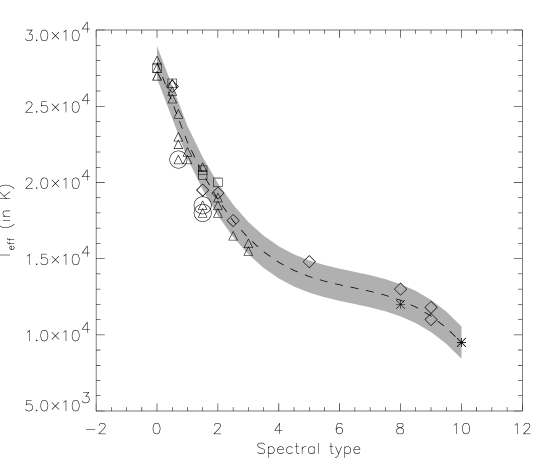
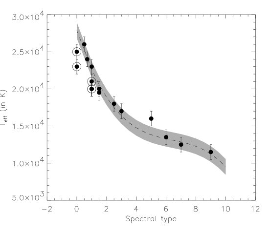
Figure 8: Left: Comparison of effective temperatures as derived in the present study with data from similar investigations. Diamonds - our data; triangles - data from Crowther et al. (2006); squares - Urbaneja (2004); asterisks - Przybilla et al. (2006). Large circles mark the three objects with strongest winds, which simultaneously show the largest deviation in $T_{\rm eff}$ from the mean (all from the sample by Crowther et al.). The dashed line represents a 3rd order polynomial fit to the data accounting for the individual errors in $T_{\rm eff}$ , and the grey-shaded area denotes the corresponding standard deviation. Spectral types refer to B-stars (i.e., “-1” corresponds to O9, and “10” to A0).
Right: $T_{\rm eff}$ estimates for GROUP I stars from Lefever et al. (2007), as a function of spectral type. The error bars correspond to $\pm$1 000 K, and the dashed line/shaded area refer to the fit on the left. Large circles mark data points which deviate significantly from this regression (see text).

A comparison of present results with such from previous studies (Crowther et al. 2006; Barlow & Cohen 1977) for three stars in common indicates that the parameters derived by Crowther et al. (2006) for HD 190 603 and HD 198 478 are similar to ours (accounting for the fact that higher $T_{\rm eff}$ and M_V result in larger $\log g$ and $\dot{M}$, respectively, and vice versa). The mass-loss rates from Barlow & Cohen (1977) (derived from the IR-excess!) for HD 198 478 and HD 202 850, on the other hand, are significantly larger than ours and those from Crowther et al., a problem already faced by Kudritzki et al. (1999) in a similar (though more simplified) investigation. This might be either due to certain inconsistencies in the different approaches, or might point to the possibility that the IR-forming region of these stars is more heavily clumped than the H_α forming one.

5 The $T_{\rm eff}$  scale for B-SGs – comparison with other investigations

5.1 Line-blanketed analyses

Besides the present study, two other investigations have determined the effective temperatures of Galactic B-type SGs by methods similar to ours, namely from Silicon and Helium (when possible) ionisation balances, employing state of the art techniques of quantitative spectroscopy on top of high resolution spectra covering all strategic lines. Crowther et al. (2006) have used the non-LTE, line blanketed code CMFGEN (Hillier & Miller 1998) to determine $T_{\rm eff}$ of 24 supergiants (luminosity classes Ia, Ib, Iab, Ia+) of spectral type B0-B3 with an accuracy of $\pm$1 000 K, while Urbaneja (2004) employed FASTWIND (as done here) and determined effective temperatures of five early B (B2 and earlier) stars of luminosity classes Ia/Ib with an (internal) accuracy of $\pm$500 K. In addition, Przybilla et al. (2006) have recently published very precise temperatures (typical error of $\pm$200 K) of four BA SGs (among which one B8 and two A0 stars), again derived by means of a line-blanketed non-LTE code, in this case in plane-parallel geometry neglecting wind effects.

Motivated by the good correspondence between data from FASTWIND and CMFGEN (which has also been noted by Crowther et al. 2006), we plotted the effective temperatures of all four investigations, as a function of spectral type (left panel of Fig. 8). Overplotted (dashed line) is a 3rd order polynomial regression to these data, accounting for the individual errors in $T_{\rm eff}$ , as provided by the different investigations. The grey-shaded area denotes the standard deviation of the regression. Obviously, the correspondence between the different datasets is (more than) satisfactory: for a given spectral subtype, the dispersion of the data does not exceed $\pm$1000 K. There are only three stars (marked with large circles), all from the sample of Crowther et al., which make an exception, showing significantly lower temperatures: HD 190 603, HD 152 236 and HD 2 905. Given their strong P Cygni profiles seen in H_α and their high luminosities - note that the first two stars are actually hypergiants - this result should not be a surprise though (higher luminosity $\rightarrow$ denser wind $\rightarrow$ stronger wind blanketing $\rightarrow$ lower $T_{\rm eff}$ ).

Very recently, Lefever et al. (2007) published a study with the goal to test whether the variability of a sample of 28 periodically pulsating, Galactic B-type SGs is compatible with opacity driven non-radial pulsations. To this end, they analysed this sample plus 12 comparison objects, also by means of FASTWIND, thus providing additional stellar and wind parameters of such objects. In contrast to both our investigation and those mentioned above, Lefever et al. could not use the Si (He) ionisation balance to estimate $T_{\rm eff}$ , but had to rely on the analysis of one ionisation stage alone, either Si II or Si III, plus two more He I lines ($\lambda$4471 and $\lambda$6678). The reason for doing so was the (very) limited spectral coverage of their sample (though at very high resolution), with only one representative Silicon ionisation stage observed per object.

Given the problems we faced during our analysis (which only appeared because we had a much larger number of lines at our disposal) and the fact that Lefever et al. were not able to independently estimate Si abundances and $v_{\rm mic}$ of their sample stars (as we have done here), the results derived during this investigation are certainly prone to larger error bars than those obtained by methods where all strategic lines could be included (see Lefever et al. for more details).

The right-hand panel of Fig. 8 displays their temperature estimates for stars from the so-called GROUP I (most precise parameters), overplotted by our regression from the left panel. The error bars correspond to $\pm$1 000 K quoted by the authors as a nominal error. While most of their data are consistent (within their errors) with our regression, there are also objects (marked again with large circles) which deviate significantly.

Interestingly, all outliers situated below the regression are stars of early subtypes (B0/B1), which furthermore show P Cygni profiles with relatively strong emission components in H_α (except for HD 15 043 which exhibits H_α in absorption), a situation that is quite similar to the one observed on the left of this figure. (We return to this point in the next section.)

On the other hand, there are two stars of B5-type with same $T_{\rm eff}$ , which lie above the regression, i.e., seem to show “overestimated” temperatures. The positions of these stars within the $T_{\rm eff}$ -spectral type plane have been extensively discussed by Lefever et al. (2007) who suggested that the presence of a radially stratified micro-turbulent velocity (as also discussed by us) or a Si abundance being lower than adopted (solar) might explain the overestimate (if so) of their temperatures. Note, however, that the surface gravity of HD 108 659 (=2.3), one of the Lefever et al. B5 targets, seems to be somewhat large for a SG but appropriate for a bright giant. Thus, it might still be that the “overestimated” temperature of HD 108 659 is a result of its misclassification as a SG whilst actually it is a bright giant. This possibility, however, cannot be applied to the other B5 target, HD 102 997, which has $\log g$ of 2.0 (and M_V of -7.0), i.e., is consistent with its classification as a supergiant.

Interestingly, the surface gravity of “our” B5 star, HD 191 243 ($\log g$ =2.6), appears also to be larger than what is typical for a supergiant of B5 subtype. With a distance modulus of 2.2 kps (Humphreys 1978), the absolute magnitude of HD 191 243 would be more consistent with a supergiant classification, but with d=1.75 kpc (Garmany & Stencel 1992) a luminosity class II is more appropriate. Thus, this star also seems to be misclassified.

Figure 9: Differences between “unblanketed” and “blanketed” effective temperatures for the combined sample (this work, Urbaneja 2004, Crowther et al. 2006, Przybilla et al. 2006 and GROUP I objects from Lefever et al. 2007), as a function of spectral type (left panel) and as a function of $\log Q$ for individual subtypes, B0 to B3 (right panel). Unblanketed $T_{\rm eff}$  are from McErlean et al. (1999).
Left: Large circles denote the same objects as in Fig. 8. The data point indicating a significant negative temperature difference corresponds to the two B5 stars (at same temperature) from the Lefever et al. sample.
Right: The size of the symbols corresponds to the size of the peak emission seen in H_α . Filled circles mark data from CMFGEN, open circles those from FASTWIND.

5.2 Temperature revisions due to line-blanketing and wind effects

In order to estimate now the effects of line-blocking/blanketing together with wind effects in the B supergiant domain (as has been done previously for the O-star domain, e.g., Markova et al. 2004; Repolust et al. 2004; Martins et al. 2005), we have combined the different datasets as discussed above into one sample, keeping in mind the encountered problems.

Figure 9, left panel, displays the differences between “unblanketed” and “blanketed” effective temperatures for this combined sample, as a function of spectral type. The “unblanketed” temperatures have been estimated using the $T_{\rm eff}$ -Spectral type calibration provided by McErlean et al. (1999), based on unblanketed, plane-parallel, NLTE model atmosphere analyses. Objects enclosed by large circles are the same as in Fig. 8, i.e., three from the analysis by Crowther et al., and seven from the sample by Lefever et al. As to be expected and as noted by previous authors on the basis of smaller samples (e.g., Crowther et al. 2006; Lefever et al. 2007), the “blanketed” temperatures of Galactic B-SGs are systematically lower than the “unblanketed” ones. The differences range from about zero to roughly 6 000 K, with a tendency to decrease towards later subtypes (see below for further discussion).

The most remarkable feature in Figure 9 is the large dispersion in $\Delta$$T_{\rm eff}$ for stars of early subtypes, B0-B3. Since the largest differences are seen for stars showing P Cygni profiles with a relatively strong emission component in H_α , we suggest that most of this dispersion is related to wind effects.

To investigate this possibility, we have plotted the distribution of the $\Delta$$T_{\rm eff}$ -values of the B0-B3 object as a function of the distant-invariant optical depth parameter $\log Q$ (cf. Sect. 4). Since the H_α emission strength does not depend on $Q$ alone but also on $T_{\rm eff}$ - for same $Q$-values cooler objects have more emission due to lower ionisation - stars with individual subclasses were studied separately to diminish this effect. The right-hand panel of Fig. 9 illustrates our results, where the size of the circles corresponds to the strength of the emission peak of the line. Filled symbols mark data from CMFGEN, and open ones data from FASTWIND. Inspection of these data indicates that objects with stronger H_α emission tend to show larger log $Q$-values and subsequently higher $\Delta$$T_{\rm eff}$ - a finding that is model independent. This tendency is particularly evident in the case of B1 and B2 objects. On the other hand, there are at least three objects which appear to deviate from this rule, but this might still be due to the fact that the temperature dependence of $Q$ has not been completely removed (of course, uncertainties in $\beta$, $T_{\rm eff}$ and $\log g$ can also contribute). All three stars (HD 89 767, HD 94 909 (both B0) and HD 154 043 (B1)) are from the Lefever et al. sample and do not exhibit strong H_α emission but nevertheless the highest $\Delta$$T_{\rm eff}$ among the individual subclasses.

In summary, we suggest that the dispersion in the derived effective temperature scale of early B-SGs is physically real and originates from wind effects. Moreover, there are three stars from the Lefever et al. GROUP I sample (spectral types B0 to B1) whose temperatures seem to be significantly underestimated, probably due to insufficient diagnostics. In our follow-up analysis with respect to wind-properties, we will discard these “problematic” objects to remain on the “conservative” side.

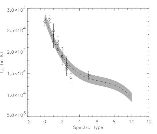
Figure 10: Temperature scale for Galactic B-SG as derived in the present study (dashed, see text), compared to $T_{\rm eff}$ estimates for similar stars in the SMC (from Trundle et al. 2004 (diamonds) and Trundle et al. 2005 (triangles)). The grey area denotes the standard deviation of the regression for Galactic objects. Spectral types account for metallicity effects (from Lennon 1997), see text.

5.3 Comparison of the temperature scales of Galactic and SMC B supergiants

Wanted to obtain an impression of the influence of metallicity on the temperature scale for B-type SGs, by comparing Galactic with SMC data. To this end, we derived a $T_{\rm eff}$ -Spectral type calibration for Galactic B-SGs on basis of the five datasets discussed above, discarding only those (seven) objects from the Lefever et al. sample where the temperatures might be particularly affected by strong winds or other uncertainties (marked by large circles in Fig, 8, right). Accounting for the errors in $T_{\rm eff}$, we obtain the following regression (for a precision of three significant digits)

$$T_{\rm eff}\,=\,27\,800\,-\,6\,000\,{\rm SP}\,+\,878\,{\rm SP}^{2}\,-\,45.9\,{\rm SP}^{3},$$ (1)

where “SP” (0-9) gives the spectral type (from B0 to B9), and the standard deviation is $\pm$1040 K. This regression was then compared to $T_{\rm eff}$ estimates obtained by Trundle et al. (2004) and Trundle et al. (2005) for B-SGs in the SMC.

We decided to compare with these two studies only, because Trundle et al. have used a similar (2004) or identical (2005) version of FASTWIND as we did here, i.e., systematic, model dependent differences between different datasets can be excluded and because the metallicity of the SMC is significantly lower than in the Galaxy, so that metallicity dependent effects should be maximised.

The outcome of our comparison is illustrated in Fig. 10: In contrast to the O-star case (cf. Massey et al. 2004, 2005; Mokiem et al. 2006), the data for the SMC stars are, within their errors, consistent with the temperature scale for their Galactic counterparts. This result might be interpreted as an indication of small or even negligible metallicity effects (both directly, via line-blanketing, and indirectly, via weaker winds) in the temperature regime of B-SGs, at least for metallicities in between solar and SMC (about 0.2 solar) values. Such an interpretation would somewhat contradict our findings about the strong influence of line-blanketing in the Galactic case (given that these effects should be lower in the SMC), but might be misleading since Trundle et al. (2004, 2005) have used the spectral classification from Lennon (1997), which already accounts for the lower metallicity in the SMC. To check the influence of this re-classification, we recovered the original (MK) spectral types of the SMC targets using data provided by Lennon (1997, Table 2), and subsequently compared them to our results for Galactic B-SGs. Unexpectedly, SMC objects still do not show any systematic deviation from the Galactic scale but are, instead, distributed quite randomly around the Galactic mean. Most plausibly, this outcome results from the large uncertainty in spectral types as determined by Azzopardi & Vigneau (1975), such that metallicity effects cannot become apparent for the SMC objects considered here. Nevertheless, we can also conclude that the classification by Lennon (1997) has been done in a perfect way, namely that Galactic and SMC stars of similar spectral type also have similar physical parameters, as expected.

Figure 11: Left: WLR for Galactic B-SGs, based on data from the combined sample: diamonds - our data; triangles - data from Crowther et al. (2006); squares - data from Urbaneja (2004) and plus signs - data from Lefever et al. (2007) (GROUP I, without the three “problematic” objects). The two pairs of symbols connected with dashed lines correspond to the two entries for HD 190 603 and HD 198 478 as listed in Table 2. For the latter object and for HD 199 478, we also provide error bars indicating the rather large uncertainty in their wind-momenta. Specially marked objects are discussed in the text.
Right: Wind-momenta of B-SGs from the left (diamonds and asterisks) are compared with similar data for O-SGs (triangles). Filled diamonds indicate B-type objects with $T_{\rm eff}$ $\geq$21 000 K, asterisks such with $T_{\rm eff}$ $\leq$12 500 K and open diamonds B-types with temperatures in between 12 500 and 21 000 K. The high luminosity solution for HD 190 603 is indicated by a square. Overplotted are the early/mid B - (small plus-signs) and A SG (large plus-signs) data derived by KPL99 and the theoretical predictions from Vink et al. (2000) for Galactic SGs with 27 500$\leq$$T_{\rm eff}$ $\leq$50 000 (dashed-dotted) and with 12 500$\leq$$T_{\rm eff}$ $\leq$ 22 500 (dashed)
Error bars provided in the lower-right corner of each panel represent the typical errors in $\log L/L_{\odot}$ and $\log D_{\rm mom}$ for data from our sample. Maximum errors in $\log D_{\rm mom}$ are about 50% larger.

6 Wind-momentum luminosity relationship

6.1 Comparison with results from similar studies

Using the stellar and wind parameters, the modified wind momenta can be calculated (Table 3, column 14), and the wind-momentum luminosity diagram constructed. The results for the combined sample (to improve the statistics, but without the “problematic” stars from the Lefever et al. GROUP I sample) are shown on the left of Figure 11. Data from different sources are indicated by different symbols. For HD 190 603 and HD 198 478, both alternative entries (from Table 2) are indicated and connected by a dashed line. Before we consider the global behaviour, we first comment on few particular objects.

$\bullet$ The position of HD 190 603 corresponding to $B-V$=0.540 (lower luminosity) appears to be more consistent with the distribution of the other data points than the alternative position with $B-V$=0.760. In the following, we give more weight to the former solution.

$\bullet$ The positions of the two B5 stars suggested as being misclassified (HD 191 243 and HD 108 659, large diamonds) fit well the global trend of the data, implying that these bright giants do not behave differently from supergiants.

$\bullet$ The minimum values for the wind momentum of HD 198 478 (with $v_{\infty}$ =200 km s^-1 ) deviate strongly from the global trend, whereas the maximum ones ($v_{\infty}$ =470 km s^-1 ) are roughly consistent with this trend. For our follow-up analysis, we discard this object because of the very unclear situation.

$\bullet$ HD 152 236 (from the sample of Crowther et al., marked with a large circle) is a hypergiant with a very dense wind, for which the authors adopted $R_{\star}$ = 112 $R_{\odot}$ , which makes this object the brightest one in the sample.

Global features.

From the left of Figure 11, we see that the lower luminosity B-supergiants seem to follow a systematically lower WLR than their higher luminosity counterparts, with a steep transition between both regimes located in between $\log L/L_{\odot}$ =5.3 and $\log L/L_{\odot}$ = 5.6. (Admittedly, most of the early type (high L) objects are Ia’s, whereas the later types concentrate around Iab’s with few Ia/Ib’s.) This finding becomes even more apparent when the WLR is extended towards higher luminosities by including Galactic O supergiants (from Repolust et al. 2004; Markova et al. 2004; Herrero et al. 2002), as done on the right of the same figure.

KPL99 were the first to point out that the offsets in the corresponding WLR of OBA-supergiants depend on spectral type, being strongest for O-SGs, decreasing from B0-B1 to B1.5-B3 and increasing again towards A supergiants. While some of these results have been confirmed by recent studies, others have not (Crowther et al. 2006; Lefever et al. 2007).

To investigate this issue in more detail and based on the large sample available now, we have highlighted the early objects (B0-B1.5, 21 000$\leq$$T_{\rm eff}$ $\leq$27 500 K) in the right-hand panel of Figure 11 using filled diamonds. (Very) Late objects with $T_{\rm eff}$ $\leq$ 12 500 K have been indicated by asterisks, and intermediate temperature objects by open diamonds. Triangles denote O-SGs. Additionally, the theoretical predictions by Vink et al. (2000) are provided via dashed-dotted and dashed lines, corresponding to the temperature regimes of O and B-supergiants, respectively (from here on referred to as “higher” and “lower” temperature predictions). Indeed,

$\bullet$ O-SGs show the strongest wind momenta, determining a different relationship than the majority of B-SGs (see below).

$\bullet$ the wind momenta of B0-B1.5 subtypes are larger than those of B1.5-3, and both follow a different relationship. However, a direct comparison with KPL99 reveals a large discrepancy for mid B1.5-B3 subtypes ($\Delta$$\log D_{\rm mom}$ about 0.5 dex), while for B0-B1.5 subtypes their results are consistent with those from our combined dataset.

$\bullet$ Late B4-B9 stars follow the same relationship as mid subtypes.

Thus, the only apparent disagreement with earlier findings relates to the KPL99 mid-B types, previously pointed out by Crowther et al. (2006), and suggested to be a result of line blocking/blanketing effects not accounted for in the KPL99 analysis. After a detailed investigation of this issue for one proto-typical object from the KPL99 sample (HD 42 087), we are convinced that the neglect of line blocking/blanketing cannot solely account for such lower wind momenta. Other effects must also contribute, e.g., overestimated $\beta$-values, though at least the latter effect still leaves a considerable discrepancy.

On the other hand, a direct comparison of the KPL99 A-supergiant dataset (marked with large plus-signs on the right of Fig. 11) with data from the combined sample shows that their wind momenta seem to be quite similar to those of mid and late B subtypes. Further investigations based on better statistics are required to clarify this issue.

6.2 Comparison with theoretical predictions and the bistability jump

According to the theoretical predictions by Vink et al. (2000), Galactic supergiants with effective temperatures between 12 500 and 22 500 K (spectral types B1 to B9) should follow a WLR different from that of hotter stars (O-types and early B subtypes), with wind momenta being systematically larger. From Figure 11 (right), however, it is obvious that the observed behaviour does not follow these predictions. Instead, the majority of O-SGs (triangles – actually those with H_α in emission, see below) follow the low-temperature predictions (dashed line), while most of the early B0-B1.5 subtypes (filled diamonds) are consistent with the high-temperature predictions (dashed-dotted), and later subtypes (from B2 on, open diamonds) lie below (!), by about 0.3 dex. Only few early B-types are located in between both predictions or close to the low-temperature one.

The offset between both theoretical WLRs has been explained by Vink et al. (2000) due to the increase in mass-loss rate at the bi-stability jump (more lines from lower iron ionization stages available to accelerate the wind), which is only partly compensated by a drop in terminal velocity. The size of the jump in $\dot{M}$, about a factor of five, was determined requiring a drop in $v_{\infty}$ by a factor of two, as extracted from earlier observations (Lamers et al. 1995).

However, more recent investigations (Crowther et al. 2006, see also Evans et al. 2004) have questioned the presence of such a “jump” in $v_{\infty}$ , and argued in favour of a gradual decrease in $v_{\infty}$ /$v_{\rm esc}$ , from $\sim$3.4 above 24 kK to $\sim$1.9 below 20 kK.

In the following, we comment on our findings regarding this problem in some detail, (i) because of the significant increase in data (also at lower $T_{\rm eff}$ ), (ii) we will tackle the problem by a somewhat modified approach and (iii) recently a new investigation of the bistability jump by means of radio mass-loss rates has been published (Benaglia et al. 2007) which gives additional impact and allows for further comparison/conclusions.

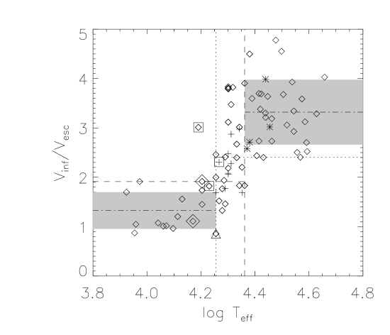
Figure 12: Ratio of $v_{\infty}$ /$v_{\rm esc}$ as a function of log $T_{\rm eff}$ . Diamonds: combined OBA-supergiant sample as in Fig. 11, right panel. Asterisks/plus-signs refer to the early/mid B supergiants from the sample by KPL99. Large diamonds again correspond to the potentially misclassified B5-objects HD 191 243 and HD 108 659. The triangle denotes the hypergiant HD 152 236 and the three squares - the various positions of HD 53 138 as derived by Crowther et al. (2006), Lefever et al. (2007) and KPL99 (references ordered by increasing $T_{\rm eff}$ ). Individual errors extend from 33% to 43%. See text.

First, let us define the “position” of the jump by means of the $v_{\infty}$ /$v_{\rm esc}$ -ratios from the OBA-supergiant sample as defined in the previous section (excluding the “uncertain” object HD 198 478). In Figure 12, two temperature regimes with considerably different values of such ratios have been identified, connected by a transition zone. In the high temperature regime ($T_{\rm eff}$ $>$ 23 kK), our sample provides $v_{\infty}/v_{\rm esc}\approx 3.3\pm 0.7$, whereas in the low temperature one ($T_{\rm eff}$ $<$ 18 kK), we find $v_{\infty}/v_{\rm esc}\approx 1.3\pm 0.4$. (Warning: The latter estimate has to be considered cautiously, due to the large uncertainties at the lower end where $v_{\infty}=v_{\rm esc}$ has been adopted for few stars due to missing diagnostics.) Note that the individual errors for $v_{\infty}/v_{\rm esc}$ are fairly similar, of the order of 33% (for $\Delta$M_V = 0.3, $\Delta$$\log g$ = 0.15 and $\Delta$$v_{\infty}$ /$v_{\infty}$ = 0.25) to 43% (in the most pessimistic case $\Delta$M_V = 1.0), similar to the corresponding Fig. 8 by Crowther et al..

In the transition zone, a variety of ratios are present, thus supporting the findings discussed above. Obviously though, large ratios typical for the high temperature region are no longer present from the centre of the transition region on, so we can define a “jump temperature” of $T_{\rm eff}$ $\approx$ 20,000 K. Nevertheless, we have shifted the border of the high-temperature regime to $T_{\rm eff}$ = 23kK, since at least low ratios are present until then (note the dashed vertical and horizontal lines in Fig. 12). The low temperature border has been defined analogously, as the coolest location with ratios $>2$ (dotted lines).

By comparing our (rather conservative) numbers with those from the publications as cited above, we find a satisfactory agreement, both with respect to the borders of the transition zone as well as with the average ratios of $v_{\infty}$ /$v_{\rm esc}$ . In particular, our high temperature value is almost identical to that derived by Crowther et al. (2006); Kudritzki & Puls 2000 provide an average ratio of 2.65 for $T_{\rm eff}$ $>$ 21 kK), whereas in the low temperature regime we are consistent with the latter investigation (Kudritzki & Puls: 1.4). The somewhat larger value found by Crowther et al. results from missing latest spectral subtypes.

Having defined the behaviour of $v_{\infty}$, we investigate the behaviour of $\dot{M}$ , which is predicted to increase more strongly than $v_{\infty}$ decreases. As we have already seen from the WLR, this most probably is not the case for a statistically representative sample of “normal” B-SGs, but more definite statements become difficult for two reasons. First, both the independent ($\log L$) and the dependent ($\log D_{\rm mom}$ ) variable depend on $R_{\star}$ (remember, the fit quantity is not $\dot{M}$ but $Q$), which is problematic for Galactic objects. Second, the wind-momentum rate is a function of $L$ but not of $T_{\rm eff}$ alone, such that a division of different regimes becomes difficult. To avoid these problems, let us firstly recapitulate the derivation of the WLR, to see the differences compared to our alternative approach formulated below.

From the scaling relations of line-driven wind theory, we have

$$\dot{M} \propto k^{\frac{1}{\alpha^{\prime}}}L^{\frac{1}{\alpha^{\prime}}}(M_{\star}(1-\Gamma))^{1-\frac{1}{\alpha^{\prime}}}$$ (2)

$$v_{\infty} = C_{\infty}v_{\rm esc},\qquad v_{\rm esc}\propto(M_{\star}(1-\Gamma))^{\frac{1}{2}}$$ (3)

where $\alpha^{\prime}$ is the difference between the line force multipliers $\alpha-\delta$ (corresponding to the slope of the line-strength distribution function and the ionisation parameter; for details, see Puls et al. 2000), $k$ - the force-multiplier parameter proportional to the effective number of driving lines and $\Gamma$ - the (distance independent!) Eddington parameter. Note that the relation for $\dot{M}$ is problematic because of its mass-dependence, and that $\dot{M}$ itself depends on distance. By multiplying with $v_{\infty}$ and ($R_{\star}$ /$R_{\odot}$ )^1/2, we obtain the well-known expression for the (modified) wind-momentum rate,

$$D_{\rm mom} = \dot{M}v_{\infty}(R_{\star}/R_{\odot})^{\frac{1}{2}}\propto k^{\frac{1}{\alpha^{\prime}}}C_{\infty}L^{\frac{1}{\alpha^{\prime}}}(M_{\star}(1-\Gamma))^{-\varepsilon}$$ (4)

$$\varepsilon = \frac{1}{\alpha^{\prime}}-\frac{3}{2}$$ (5)

$$\log D_{\rm mom} \approx \frac{1}{\alpha^{\prime}}\log L+D_{0}$$ (6)

$$D_{0} = \frac{1}{\alpha^{\prime}}\log k+\log C_{\infty}+{\rm const}$$ (7)

where we have explicitly included here those quantities which are dependent on spectral type (and metallicity). Remember that this derivation assumes the winds to be unclumped, and that $\varepsilon$ is small, which is true at least for O-supergiants (Puls et al. 2000).

Investigating various possibilities, it turned out that the (predicted) scaling relation for a quantity defined similarly as the optical-depth invariant is particularly advantageous:

$$Q^{\prime} =: \frac{\dot{M}}{R_{\star}^{\frac{3}{2}}}\frac{g_{\rm eff}}{v_{\infty}}\propto\frac{k^{\frac{1}{\alpha^{\prime}}}}{C_{\infty}}T_{\rm eff}^{\frac{4}{\alpha^{\prime}}}g_{\rm eff}^{-\varepsilon},\qquad g_{\rm eff}\propto\frac{M_{\star}(1-\Gamma)}{R_{\star}^{2}}$$ (8)

$$\log Q^{\prime} \approx \frac{4}{\alpha^{\prime}}\log T_{\rm eff}+D_{0}^{\prime}$$ (9)

$$D_{0}^{\prime} = \frac{1}{\alpha^{\prime}}\log k-\log C_{\infty}+{\rm const^{\prime}}$$ (10)

Figure 13: Modified optical depth invariant, $\log Q^{\prime}$ (Eq. 8, as a function of log $T_{\rm eff}$ . Symbols as in Fig. 12, with vertical bars indicating the “transition” region between 18 and 23 kK. Note that the mid B-type supergiants from the KPL99 sample (plus-signs) deviate from the trend displayed by the other objects. Regression for the complete sample (excluding HD 53 138, HD 152 236 and the KPL99 B-supergiants) overplotted in solid; dashed regression similar, but additionally excluding the objects in the transition region (see text).

This relation for the distance independent quantity $Q^{\prime}$ becomes a function of log $T_{\rm eff}$ and $D_{0}^{\prime}$ alone if $\alpha^{\prime}$ were exactly 2/3, i.e., under the same circumstances as the WLR. Obviously, this relation has all the features we are interested in, and we will investigate the temperature behaviour of $\dot{M}$ by plotting log $Q^{\prime}$ vs. log $T_{\rm eff}$ . We believe that the factor $v_{\infty}/g_{\rm eff}$ is a monotonic function on both sides of and through the transition zone, as is also the case for $g_{\rm eff}$ itself. Thus, the $\log Q^{\prime}-\log T_{\rm eff}$ relation should react only on differences in the effective number of driving lines and on the different ratio $v_{\infty}$ /$v_{\rm esc}$ on both sides of the transition region.

Fig. 13 displays our final result. At first glance, there is almost no difference between the relation on both sides of the “jump”, whereas inside the transition zone there is a large scatter, even if not accounting for the (questionable) mid-B star data from KPL99.

Initially, we calculated the average slope of this relation by linear regression, and then the corresponding slope by additionally excluding the objects inside the transition region (dashed). Both regressions give similar results, interpreted in terms of $\alpha^{\prime}$ with values of 0.65 and 0.66 (!), respectively, and with standard errors regarding $\log Q^{\prime}$ of $\pm 0.33$ and $\pm 0.28$ dex.

If the relations indeed were identical on both sides of the jump, we would also have to conclude that the offset, $D_{0}^{\prime}$, is identical on both sides of the transition region. In this case, the decrease in $v_{\infty}$ /$v_{\rm esc}$ within the transition zone has to be more or less exactly balanced by the same amount of a decrease in $k^{\frac{1}{\alpha^{\prime}}}$, i.e., both $\dot{M}$ and $v_{\infty}$ are decreasing in parallel, in complete contradiction to the prediction by Vink et al.

A closer inspection of Fig. 13 (in combination with the corresponding WLR of Fig. 11) implies an alternative interpretation. At the hottest (high luminosity) end, we find the typical division of supergiants with H_α in emission and absorption, where the former display an offset of a factor 2…3 above the mean relation, a fact which has been interpreted to be related to wind-clumping previously.

Proceeding towards lower temperatures, the $Q^{\prime}$ relation becomes well defined between roughly 31kK and the hot side of the transition zone (in contrast to the WLR, which shows more scatter, presumably due to uncertain $R_{\star}$ ). Inside the transition zone and also in the WLR around $\log L/L_{\odot}$ $\approx$ 5.45, a large scatter is present, followed by an apparent steep decrease in $\log Q^{\prime}$ and wind-momentum rate, where the former is located just at the “jump temperature” of 20 kK. Note that the mid-B type objects of the KPL99 sample are located just in this region. From then on, $Q^{\prime}$ appears to remain almost constant until 14 kK, whereas the WLR is rather flat between 5.1 $<$ $\log L/L_{\odot}$ $<$ 5.4, in agreement with the findings by Benaglia et al. (2007, their Fig. 8). At the lowest temperatures/luminosities, both $Q^{\prime}$ and the WLR decrease again, with a similar slope as in the hot star domain. This offers a possibility of a discontinuous behaviour, but, again, in contradiction to what is predicted.

We now quantify the behaviour of the mass-loss rate in the low temperature region (compared to the high temperature one), in a more conservative manner than estimated above, by using both the $\log Q^{\prime}$ relation and the WLR. Accounting for the fact that the corresponding slopes are rather similar on both sides of the transition zone, we define a difference of offsets,

$$\Delta D_{0} \approx \frac{1}{\alpha^{\prime}}\Delta\log k+\Delta\log C_{\infty}$$ (11)

$$\Delta D_{0}^{\prime} \approx \frac{1}{\alpha^{\prime}}\Delta\log k-\Delta\log C_{\infty},$$ (12)

evaluated with respect to “low” minus “high”. From the WLR, we have $\Delta D_{0}<0$, whereas the $Q^{\prime}$ relation implies $\Delta D_{0}^{\prime}\geq 0$, to be cautious. Thus, the change in $\frac{1}{\alpha^{\prime}}\Delta\log k$ (which expresses the difference in log $\dot{M}$ on both sides of the jump, cf. Eq. 2) is constrained by

$$\Delta\log C_{\infty}\leq\frac{1}{\alpha^{\prime}}\Delta\log k<-\Delta\log C_{\infty}.$$ (13)

To be cautious again, we note that $\Delta\log C_{\infty}$ should lie in the range log(1.9/2.4) … log(1.3/3.3) = -0.1 … -0.4, accounting for the worst and the average situation (cf. Fig. 12).

Thus, the scaling factors of mass-loss rates on both sides of the jump (cool vs. hot) differ by

$$0.4{\ldots}0.8\leq k^{\frac{1}{\alpha^{\prime}}}<1.25{\ldots}2.5$$ (14)

i.e., $\dot{M}$ either decreases in parallel with $v_{\infty}$ /$v_{\rm esc}$ or increases marginally.

Wind efficiencies.

Before discussing the implications of these findings, let us come back to the investigations by Benaglia et al. (2007) who recently reported evidence of the possible presence of a local maximum in the wind efficiency, $\eta$ = $\dot{M}$ $v_{\infty}$ /(L/c), around 21 000 K, which would be at least in qualitative agreement with theoretical predictions. In Figure 14, we compare the wind-efficiencies as derived for our combined sample (from H_α ) to corresponding data from their radio measurements (filled dots). The dashed line in the figure displays the theoretical predictions, which, again, are based on the models by Vink et al. (2000).

Figure 14: Wind-efficiency, $\eta$, as a function of $T_{\rm eff}$ , for our combined sample (symbols as in Fig. 12) and objects as analysed by Benaglia et al. 2007 (filled dots, mass-loss rates from radio excess). Eight objects in common have been discarded from the latter sample. Overplotted (dashed) are their theoretical predictions, based on the models by Vink et al. (2000).

There are eight stars in common with our sample for which we display the H_α results only, not to artificially increase the statistics. At least for five of those, all of spectral type B0 to B2, a direct comparison of the H_α and radio results is possible, since same values of $T_{\rm eff}$ , $R_{\star}$ and $v_{\infty}$ have been used to derive the corresponding wind efficiencies. In all but one of these stars, radio and optical mass-loss rates agree within 0.2 dex, which is comparable to the typical uncertainty of the optical data. Translated to potential wind-clumping, this would mean that the outer and inner wind-regions were affected by similar clumping factors, in analogy to the findings for thin O-star winds (Puls et al. 2006). From Fig. 14 now, several issues are apparent:

$\bullet$ As for the wind-momenta and mass-loss rates, also the wind-efficiencies of OB-supergiants do not behave as predicted, at least globally. Instead, they follow a different trend (for $\alpha^{\prime}=2/3$, one expects $\eta\propto T_{\rm eff}^{2}\,(R_{\star}^{0.5}k^{1.5}C_{\infty})$, i.e., a parabola with spectral type dependent offset), where, as we have already seen, the offset at the cool side of the jump is much lower than in the simulations by Vink et al. Actually, this is true for almost the complete B-SGs domain (between 27 and 10 kK).

$\bullet$ Similar as in the observed wind-momentum luminosity diagram (Fig. 11, right panel), some of the O-supergiants do follow the predictions, while others show wind-efficiencies which are larger by up to a factor of two. Note that this result is supported by both H_α and radio diagnostics. If this discrepancy were interpreted in terms of small-scale clumping, we would have to conclude that the winds of these objects are moderately clumped, even at large distances from the stellar surface.

$\bullet$ Within the transition zone, a large scatter towards higher values of $\eta$ is observed, which, if not due to systematic errors in the adopted parameters, indeed might indicate the presence of a local maximum, thus supporting the findings of Benaglia et al. (2007). From a careful investigation of the distribution of stellar radii, terminal velocities and mass-loss rates, we believe that this local bump does not seem to be strongly biased by such uncertainties, but is instead due to a real increase in $\dot{M}$ .

6.3 Discussion

Regarding a comparison with theoretical models, the major conclusion to be drawn from the previous section is as follows. In addition to the well-known factor of two discrepancies for dense O-SG winds, the most notable disagreement (discarding local effects within the transition zone for the moment) is found in the low $T_{\rm eff}$ /low $L$ B-SG domain, confirming the analysis by Crowther et al. (2006). The predictions by Vink et al. clearly require the decrease in $v_{\infty}$ to be overcompensated by an increase in $\dot{M}$ throughout the complete mid/late B-star regime, whereas our analysis has shown that this is not the case. At best, $\dot{M}$ increases by the same amount as $v_{\infty}$ decreases, though a reduction of $\dot{M}$ seems to be more likely, accounting for the fact that the upper limit in Eq. 14 is a rather conservative estimate.

Since the calculation of absolute mass-loss rates and wind-momenta is a difficult task and depends on a number of uncertainties (see below), let us firstly consider the possibility that at least the predictions regarding the relative change in $\dot{M}$ (from hot to cool objects) are correct, and that clumping affects this prediction only marginally.

In this case, the most simple explanation for the detected discrepancy is that cooler objects are less clumped than hotter ones. Since Vink et al. predict an increase in $\dot{M}$ of a factor of five, this would imply that the clumping factors for hotter objects are larger by factors of 4 (most optimistic case) to 156 (worst case) compared to those of cooler ones. Given our present knowledge (see Fullerton et al. 2006, Puls et al. 2006 and references therein), this is not impossible, but raises the question about the physical origin of such a difference. This hypothesis would also imply that all B-SG mass-loss rates are overpredicted, though to a lesser extent for cooler subtypes.

In the alternative, and maybe more reasonable scenario that the clumping properties of OBA supergiants were not too different, we would have to conclude that at least the low temperature predictions suffer from unknown defects. Note, however, that a potential “failure” of these predictions does not invalidate the radiation driven wind theory itself. The actual mass-loss rates depend on the effective number of driving lines, and, at least in principle, this number should decrease towards lower $T_{\rm eff}$ , due to an increasing mismatch between the position of these lines and the flux maximum (e.g., Puls et al. 2000). In Vink’s models, it increases instead because Fe iii has many more lines than Fe iv, and because these lines are distributed over a significant spectral range. The absolute number of these lines and their strengths, however, depend on details of the available data (not forgeting the elemental abundances, Krticka & Kubat 2007), a consistent description of the ionisation/excitation equilibrium and also on other, complicating effects (e.g., the diffuse radiation field diminishing the line acceleration in the lower wind, Owocki & Puls 1999, and the potential influence of microturbulence, Lucy 2007), which makes quantitative predictions fairly ambiguous. Moreover, if the winds were clumped, this would influence the hydrodynamical simulations, due to a modified ionisation structure.

That there is an effect which is most probably related to the principal bistability mechanism (Pauldrach & Puls 1990) remains undisputed, and is evident from the more or less sudden decrease in $v_{\infty}$ /$v_{\rm esc}$ . Additionally, there is a large probability that at least inside the transition zone a “local” increase of ($\dot{M}$ $v_{\infty}$ ) is present, which would partly support the arguments by Vink et al., though not on a global scale. Furthermore, the scatter of $Q^{\prime}$ (and wind-momentum rate) turned out to be much larger in the transition region than somewhere else. This might be explained by the fact that hydrogen begins to recombine in the wind just in this region, whereas the degree of recombination depends on a multitude of parameters, thus leading to the observed variety of mass-loss rates and terminal velocities. Finally, note that at least the observed hypergiant seems to be consistent with the bistability scenario, which, after all, has been originally “invented” for these kind of objects.

7 Summary and future work

In this study, we have presented a detailed investigation of the optical spectra of a small sample of Galactic B supergiants, from B0 to B9. Stellar and wind parameters have been obtained by employing the NLTE, unified model atmosphere code FASTWIND (Puls et al. 2005), assuming unclumped winds. The major findings of our analysis can be summarised as follows.

1. We confirm recent results (Ryans et al. 2002; Dufton et al. 2006; Simon-Diaz & Herrero 2007) of the presence of a (symmetric) line-broadening mechanism in addition to stellar rotation, denoted as “macro-turbulence”. The derived values of $v_{\rm mac}$ are highly supersonic, decreasing from $\approx$ 60 km s^-1 at B0 to $\approx$ 30 km s^-1 at B9.

2. We determined the Si abundances of our sample stars in parallel with their corresponding micro-turbulent velocities.
(i) For all but one star, the estimated Si abundances were consistent with the corresponding solar value (within $\pm$0.1 dex), in agreement with similar studies (Gies & Lambert 1992; Rolleston et al. 2000; Urbaneja 2004; Przybilla et al. 2006). For HD 202 850, on the other hand, an overabundance of about 0.4 dex has been derived, suggesting that this late-B supergiant might be a silicon star.
(ii) The micro-turbulent velocities tend to decrease towards later B subtypes, from 15 to 20 km s^-1 at B0 (similar to the situation in O-supergiants) to 7 km s^-1 at B9, which is also a typical value for A-SGs.
(iii) The effect of micro-turbulence on the derived effective temperature was negligible as long as Si lines from the two major ions are used to determine it.

3. Based on our $T_{\rm eff}$ estimates and incorporating data from similar investigations (Crowther et al. 2006; Urbaneja 2004; Przybilla et al. 2006; Lefever et al. 2007), we confirm previous results (e.g., Crowther et al. 2006) on a 10% downwards revision of the effective temperature scale of early B-SGs, required after incorporating the effects of line blocking/blanketing. Furthermore, we suggest a similar correction for mid and late subtypes. When strong winds are present, this reduction can become a factor of two larger, similar to the situation encountered in O-SGs (Crowther et al. 2002).

4. To our surprise, a comparison with data from similar SMC objects (Trundle et al. 2004, 2005) did not reveal any systematic difference between the two temperature scales. This result is interpreted as an indication that the re-classification scheme as developed by Lennon (1997) to account for lower metal line strengths in SMC B-SGs also removes the effects of different degrees of line blanketing.

5. Investigating the wind properties of a statistically significant sample of supergiants with $T_{\rm eff}$ between 10 and 45 kK, we identified a number of discrepancies between theoretical predictions (Vink et al. 2000) and observations. In fair accordance with recent results (Evans et al. 2004; Crowther et al. 2006), our sample indicates a gradual decrease in $v_{\infty}$ in the bi-stability (“transition”) region, which is located at lower temperatures than predicted: 18 to 23 kK (present study) against 22.5 to 27 kK.

By means of a $newly$ defined, distance independent quantity, $Q^{\prime}=\dot{M}/R_{\star}^{1.5}\,g_{\rm eff}/v_{\infty})$ we have investigated the behaviour of $\dot{M}$ as a function of $T_{\rm eff}$ . Whereas inside the transition zone a large scatter is present (coupled with a potential local maximum in wind efficiency around 21 kK), $Q^{\prime}$ remains a well defined function with low scatter in the hot and cool temperature region outside the transition zone. Combining the behaviour of $Q^{\prime}$ and the modified wind-momentum rate, the change in $\dot{M}$ over the bi-stability jump (from hot to cool) could be constrained to lie within the factors 0.4 to 2.5, to be conservative. Thus, $\dot{M}$ either decreases in parallel with $v_{\infty}$ /$v_{\rm esc}$ (more probable), or, at most, the decrease in $v_{\infty}$ is just balanced by a corresponding increase in $\dot{M}$ (less probable). This finding contradicts the predictions by Vink et al. (2000) that the decrease in $v_{\infty}$ should be over-compensated by an increase in $\dot{M}$ , i.e., that the wind-momenta should increase over the jump. Considering potential clumping effects, we have argued that such effects will not change our basic result, unless hotter objects turn out to be substantially more strongly clumped than cooler ones. In any case, at least in the low temperature region present theoretical predictions for $\dot{M}$ are too large!

This finding is somewhat similar to the recent “weak-wind problem” for late O-dwarfs, though probably to a lesser extent. Thus, it might be that our understanding of radiation driven winds is not as complete as thought only a few years ago. Thus, it is of extreme importance to continue the effort of constructing sophisticated wind models, including the aforementioned effects (wind-clumping, diffuse radiation field, micro-turbulence), both in terms of stationary and time-dependent simulations. With respect to the objects of the present study, a re-analysis of the “peculiar” mid-type B-supergiants from the KPL99 sample is urgently required as well. Finally, let us (once more) point to the unresolved problem of macro-turbulence, which implies the presence of rather deep-seated, statistically distributed and highly supersonic velocity fields. How can we explain such an effect within our present-day atmospheric models of hot, massive stars?