Structure, Time Propagation and Dissipative Terms for Resonances

Abstract

For odd anharmonic oscillators, it is well known that complex scaling can be used to determine resonance energy eigenvalues and the corresponding eigenvectors in complex rotated space. We briefly review and discuss various methods for the numerical determination of such eigenvalues, and also discuss the connection to the case of purely imaginary coupling, which is ${\mathcal{PT}}$-symmetric. Moreover, we show that a suitable generalization of the complex scaling method leads to an algorithm for the time propagation of wave packets in potentials which give rise to unstable resonances. This leads to a certain unification of the structure and the dynamics. Our time propagation results agree with known quantum dynamics solvers and allow for a natural incorporation of structural perturbations (e.g., due to dissipative processes) into the quantum dynamics.

I INTRODUCTION

Quantum tunneling is one of the intriguing phenomena in quantum mechanics. Since the seminal work of G. Gamow on the theory of the alpha decay of a nucleus Ga1929 , quantum tunneling of a particle trapped in a metastable potential well has been studied in detail in many areas of physics. Indeed, in mathematical terms, the decay width of the corresponding resonance state in an, e.g., cubic potential can be traced back to an instanton configuration which is a solution of the classical equations of motion of a particle moving in the “inverted” potential $-V(q)$ in such a way that the classical action of the particle along its trajectory remains finite even though the time domain covered by its trajectory is the entire space $\mathbbm{R}$. Here, the instanton configuration covers the domain naturally associated with the tunneling process from a relative minimum of the potential to a point where a horizontal line would emerge from the “tunnel” potential. An approximation to the width can be obtained by considering the fluctuations around the classical path, and by a subsequent evaluation of the Fredholm determinant describing the fluctuations. This is quite analogous to the case of double-well-like potentials ZJJe2004i ; ZJJe2004ii , where the instanton configuration describes an oscillatory motion covering a trajectory oscillating between the two degenerate maxima of the inverted potential.

At the same time, the structure of the potentials depends very much on the complex phase of the coupling constant. Let us assume a metastable potential approximated by a one-dimensional harmonic oscillator perturbed by a cubic term $\sqrt{g}\,q^{3}$, where $g$ is the coupling constant. For purely imaginary $\sqrt{g}={\mathrm{i}}\beta$, with $\beta\in\mathbbm{R}$, the Hamiltonian is invariant under the composed application of a parity transformation and a time reversal and thus called $\mathcal{PT}$-symmetric. In some sense, the $\mathcal{PT}$-symmetric case is a natural generalization of hermiticity (or even self-adjointness) to the complex domain, and it will be verified here that a number of concepts known to be applicable to “stable” anharmonic oscillators are applicable to the $\mathcal{PT}$-symmetric cubic potential as well.

Coming back to the case of real coupling parameter $\sqrt{g}$, we note that known methods for the numerical determination of resonance energies and widths include the diagonalization of a complex rotated Hamiltonian matrix, Borel resummation BorelPhi4 ; BeWu1969 ; BeWu1973 in complex directions of the parameters, and strong-coupling expansions. These three methods will be discussed and contrasted here as they are important for the construction of an adiabatic, complex transformed time propagation algorithm that is also described in this article. Namely, we attempt to solve the problem of how to propagate a wave packet that moves under the influence of a potential with metastable resonances and which may thus even “escape” to the classical region of attraction where the potential assumes large negative values, without the need for a temporally adjusted numerical grid and without the need for the introduction of transparent boundary conditions. Moreover, we attempt to construct this algorithm using complex resonance eigenstates, thus giving a manifest interpretation to the complex resonance state and energies within the time propagation method, including the back-transformation of the complex rotated and propagated states to the normal coordinate representation.

This paper is organized as follows. In Sec. II, we recall some basic definitions related to the cubic potential, to perturbative and strong-coupling expansions and to the method of complex scaling. Also, corresponding numerical investigations are discussed. In Sec. III, we discuss a method for time propagation in the cubic potential, which leads to the above mentioned desired unification. Finally, a summary is presented in Sec. IV. An appendix is devoted to the discussion of potential applications of the algorithms discussed here within a solid-state physics context. In the entire article, we attempt to follow a rather detailed style in the presentation and hope that the reader will not find the level of detail excessive.

II COMPLEX RESONANCE ENERGIES VERSUS REAL $\bm{\mathcal{PT}}$–SYMMETRIC SPECTRUM FOR THE CUBIC OSCILLATOR

II.1 Orientation

Although our analysis can easily be generalized to quintic and other “odd” potentials with metastable resonances, we start for simplicity with the one–dimensional Hamiltonian of the cubic potential in the normalization

$$H_{\rm c}\,=\,-\frac{1}{2}\,\frac{\partial^{2}}{\partial q^{2}}+\frac{1}{2}\,q^{2}+\sqrt{g}\,q^{3}\,,$$ (1)

which recovers the harmonic oscillator spectrum $E_{N}=N+{\textstyle{1\over 2}}$ in the limit of a vanishing coupling constant $g\to 0$, where $N$ is a nonnegative integer and constitutes the quantum number of the state. For nonvanishing $g$, the operator (1) is not self–adjoint, and it does not possess a spectrum of discrete, real energy eigenvalues. For real and positive $g$, the cubic Hamiltonian (1) possesses resonances, i.e. poles of the resolvent $(H_{\rm c}-E)^{-1}$ which is a priori defined as a holomorphic function for ${\rm Im}\,E>0$. The poles (resonances) become apparent in the meromorphic analytic continuation of the resolvent to ${\rm Im}\,E<0$. The resonance energy eigenvalues are of the form

$$E_{N}(g)={\rm Re}[E_{N}(g)]-{\mathrm{i}}\,\frac{\Gamma_{N}(g)}{2}\,.$$ (2)

By contrast, for purely imaginary coupling $\sqrt{g}={\rm i}\,\beta$, the Hamiltonian (1) is ${\mathcal{P}T}$-symmetric, i.e. it is invariant under a simultaneous parity transformation $q\to-q$ and a time reversal operation $t\to-t$, the latter being equivalent to an explicit complex conjugation of the Hamiltonian and thus to the replacement $\beta\to-\beta$.

Based on numerical evidence, it has been conjectured around 1985 by D. Bessis and one of us (J. Z.–J.) in private communications that the spectrum of the ${\mathcal{P}T}$-symmetric Hamiltonians of odd anharmonic oscillators should consist of real eigenvalues, even if these Hamiltonians are obviously not self-adjoint. C. M. Bender and others have recently studied ${\mathcal{P}T}$-symmetric Hamiltonians quite intensively (see, e.g., Refs. BeBo1998 ; BeBoMe1999 ; BeWe2001 ; BeDuMeSi2001 ; BeBrJo2002 ). Note, in particular, that even the quartic anharmonic oscillator with negative coupling becomes a ${\mathcal{P}T}$-symmetric Hamiltonian with real spectrum when endowed with appropriate boundary conditions imposed on the wave function as a function of a complex coordinate, as detailed in Eq. (4) of Ref. BeBoJoMeSi2001 . The conjecture has recently been supported on mathematical grounds (see Refs. Sh2002cmp ; DoDuTa2001i ; DoDuTa2001ii ; DoDuTa2005 ). Important further contributions to the development of the theory of ${\mathcal{P}T}$-symmetric quantum mechanics have been summarized in Refs. BeBo1998 ; BeBoMe1999 ; BeBrJo2002 .

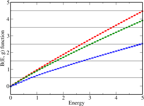
Figure 1: (color online.) Energy dependence of the function $B(E,g)$ for the $\mathcal{PT}$-symmetric case. Results are presented for the coupling parameters $\sqrt{g}={\rm i}\beta$ with $\beta=1/10$ (red circles), $\beta=1/5$ (green squares) and $\beta=1$ (blue triangles).

Table 1: Ground-state energy of the cubic Hamiltonian for the $\mathcal{PT}$-symmetric case $\sqrt{g}={\rm i}\,\beta$. Results have been obtained by the diagonalization of the complex-transformed Hamiltonian in the basis of the harmonic oscillator wavefunctions (“exact” values) and by solving the quantization condition given in Eq. (7). The apparently “converged” decimals for the solutions of $B(E,g)={\textstyle{1\over 2}}$ are underlined.

$\beta\,\,\,$	$E_{0}(g)$	Solution of $B(E,g)={\textstyle{1\over 2}}$
$1/10$	0.512 538 145	0.512 538 145
$1/8$	0.518 760 345	0.518 760 344(1)
$1/6$	0.530 781 759	0.530 781 77(1)
$1/4$	0.558 372 124	0.558 377(4)
$1/2$	0.645 877 080	0.645 7(3)

II.2 Imaginary coupling parameter and real energies

The discussion in this section is a priori relevant only for the case $\sqrt{g}={\mathrm{i}}\beta$, with $\beta\in\mathbbm{R}$, but we will keep a general $g$ in the first considerations, because the general formulas (as a function of $g$) will be useful later in this article. First, we recall that, as explained in Refs. ZJJe2004i ; ZJJe2004ii , the spectrum of anharmonic oscillators can be described in many cases by two functions $B$ and $A$. Respectively, these are related to the perturbative expansion about the minima of the potential and to the tunneling of the quantal particle from one degenerate or quasi-degenerate minimum (if it exists) to the other degenerate or quasi-degenerate minimum of the potential. Specifically, around Eq. (3.31) of Sec. 3 of Ref. ZJJe2004i , it is explained how, in the case of integrable systems, a “perturbative $B$ function” can be obtained from the perturbative expansion of the logarithmic derivative of the wave function, which fulfills a differential equation of the Riccati type and which is subject to a uniqueness condition which gives rise to the integer $N$ on the right-hand side of Eq. (4). Using techniques outlined in Ref. ZJ1984jmp , the function $B(E,g)$ can be easily determined for the cubic potential, and the first terms read as follows,

$$B(E,g) = E+g\left(\frac{7}{16}+\frac{15}{4}\,E^{2}\right)+g^{2}\left(\frac{1365}{64}\,E+\frac{1155}{16}\,E^{3}\right)+\mathcal{O}(g^{3})\,.$$ (3)

By formulating the initial perturbation as $\sqrt{g}\,q^{3}$, we have obtained a perturbative expansion for $B$ which involves integer powers in the coupling constant. As usual, the perturbative expansion for the $N$th energy level can be obtained by inverting the condition

$$B(E,g)=N+{\textstyle{1\over 2}}\,,$$ (4)

and we obtain the standard Rayleigh–Schödinger perturbation theory (RSPT) series for the $N$th level of the cubic potential,

$$E_{N}(g)=\sum\limits_{k=0}^{\infty}E^{(0)}_{N,K}\,g^{k}\,,$$ (5)

where $K$ is the order of perturbation theory, and the leading perturbative coefficients read as follows, for a general level with quantum number $N$,

$$E^{(0)}_{N,0}= \;N+{\textstyle{1\over 2}}\,,$$ (6a)

$$E^{(0)}_{N,1}= \;-\left[\frac{7}{16}+\frac{15}{4}\left(N+{\textstyle{1\over 2}}\right)^{2}\right]\,,$$ (6b)

$$E^{(0)}_{N,2}= \;-\left[\frac{1155}{64}\left(N+{\textstyle{1\over 2}}\right)+\frac{705}{16}\left(N+{\textstyle{1\over 2}}\right)^{3}\right]\,,$$ (6c)

$$E^{(0)}_{N,3}= \;-\left[\frac{101479}{2048}+\frac{209055}{256}\left(N+{\textstyle{1\over 2}}\right)^{2}+\frac{115755}{128}\left(N+{\textstyle{1\over 2}}\right)^{4}\right]\,.$$ (6d)

The minus signs are explicitly indicated to illustrate that all perturbative coefficients are negative for all levels, except for the leading term $N+{\textstyle{1\over 2}}$, which stems from the unperturbed harmonic oscillator.

If perturbation theory determines the energy eigenvalues completely in the $\mathcal{PT}$-symmetric case and there are no instanton configurations to consider, then the quantization condition (4) can be reformulated as

$$\frac{1}{\Gamma\left({\textstyle{1\over 2}}-B(E,g)\right)}=0\,,\qquad\sqrt{g}={\mathrm{i}}\,\beta.$$ (7)

This quantization condition is formulated such as to display the analogy to those for more complex potentials like the double well [see Eq. (2) of Ref. JeZJ2001 ], but it lacks the “instanton $A$ function” present in the cited equation. A Bohr–Sommerfeld quantization condition of the form (7) is relevant for stable anharmonic oscillators like, e.g., the quartic one with a perturbation proportional to $g\,q^{4}$ for positive coupling $g$, where there are no instanton configurations to consider and therefore no “instanton $A$ function” present. We now investigate to which extent this quantization condition could be relevant for the cubic anharmonic oscillator.

To this end, we first recall that the cubic Hamiltonian (1) displays ${\mathcal{P}T}$-symmetry for imaginary coupling $\sqrt{g}={\rm i}\beta$. The spectrum of the cubic oscillator becomes real in this case, as a consequence of pseudo–Hermiticity Mo2002 , and the perturbation series (5) becomes an alternating, factorially divergent series in the variable $g=-\beta^{2}$; series of this type are typically Borel-summable. We are therefore led to the conjecture that the quantization condition (7) should describe the energy levels of the cubic Hamiltonian (1), but only for the ${\mathcal{P}T}$-symmetric case $\sqrt{g}={\rm i}\beta$.

As discussed in Sec. II and as shown in our previous paper (Ref. SuLuZJJe2006 ), the direct analysis of the perturbative $B$ function which enters the quantization condition (7), without any detour via the perturbation series (5), can be used to investigate our conjecture formulated above, in order to calculate the energy eigenvalues of the cubic Hamiltonian (1) directly. Here, we explore this approach in the case of imaginary coupling $\sqrt{g}={\rm i}\beta$. To this end, we interpret $B(E,g)$ as a function of $E$ (at fixed $g$) and numerically determine the points at which this function assumes values of the form $N+{\textstyle{1\over 2}}$. According to Eq. (7), these points correspond to the real energy eigenvalues $E_{N}(g)$ of the cubic Hamiltonian in the ${\mathcal{P}T}$-symmetric case. In many cases, direct investigation of the perturbative $B$ function has proved to be numerically more stable than that of the Borel-resummed series (5) (see alse Ref. SuLuZJJe2006 ).

In Fig. 1, for example, we display $B(E,g)$ as a function of the (real) energy argument $E$ for different fixed values of the coupling parameters $g$. Specifically, we consider the cases $\sqrt{g}={\rm i}\beta={\rm i}/10$ (circles), $\sqrt{g}={\rm i}\beta={\rm i}/5$ (squares) and $\sqrt{g}={\rm i}\beta={\rm i}$ (triangles). The points where $B(E,g)=N+{\textstyle{1\over 2}}$ are clearly displayed. The (real) ground-state energy $E_{N}(g)$ for the $\mathcal{PT}$-symmetric case is presented in Table 1 and compared to reference data obtained via a diagonalization of the Hamiltonian matrix. The ground-state energy is well reproduced at $\beta=1/10$ (up to 9 decimal digits). For stronger coupling, there is a larger uncertainty in the determination of the ground–state energy value $E_{N=0}(g)$ because the power series (3) is divergent for all nonvanishing $g$, and, hence, resummation techniques are required for its calculation. In all cases, the function $B(E,g)$ is calculated by means of a generalized Borel–Páde method, similar to Ref. SuLuZJJe2006 . We observe, in higher (Borel) transformation orders, an oscillatory behaviour of the Borel integral, evaluated along complex directions, for larger $g$. These oscillations cannot be overcome when the transformation order is increased and represent a fundamental limit of the convergence of resummed weak-coupling perturbation theory in the case of a large (modulus of the) coupling parameter $g$. All numerical experiments support the conjecture (7) for the $\mathcal{PT}$-symmetric case.

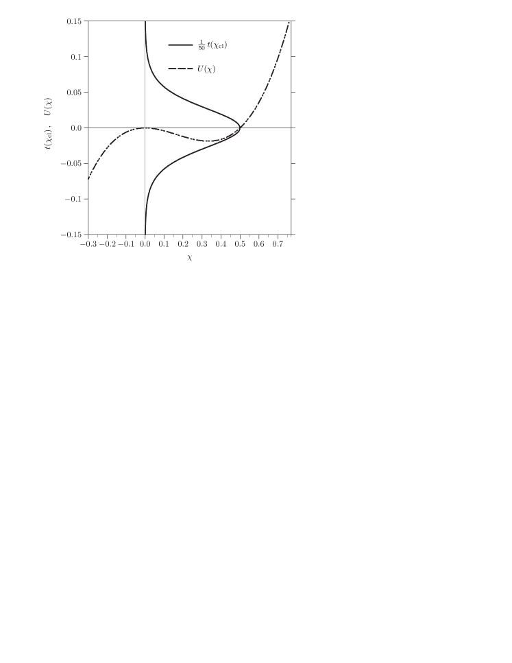
Figure 2: Instanton configuration for the cubic potential. The dashed line is the potential $U(\chi)=\chi^{3}-{\textstyle{1\over 2}}\,\chi^{2}$. The solid line is the worldline of the instanton configuration $\chi_{\rm cl}(t)=[\cosh(t)+1]^{-1}$, which reads in inverted form $t(\chi_{\rm cl})=\pm{\rm arccosh}[(1-\chi_{\rm cl})/\chi_{\rm cl}]$.

II.3 Real coupling parameter and complex resonance energies

We again consider the Hamiltonian (1), but this time for real and positive $g$. First, let us note that the structure of the perturbation series (5) is of course unaffected by a change in the complex phase of the coupling parameter. However, we now have instanton configurations to consider. Let us consider for a moment the classical Euclidean action, corresponding to (1),

$$S[q(t)]=\int{\mathrm{d}}t\,\left[\frac{1}{2}\,\left(\frac{\partial}{\partial t}q(t)\right)^{2}+\frac{1}{2}\,q(t)^{2}+\sqrt{g}\,q(t)^{3}\right]\,.$$ (8)

This action describes the motion of a particle in the potential $-\sqrt{g}\,q(t)^{3}-{\textstyle{1\over 2}}\,q(t)^{2}$. Via the change of variable $q(t)=-\chi(t)/\sqrt{g}$, we obtain the action,

$$S[\chi(t)]=\frac{1}{g}\,\int{\mathrm{d}}t\,\left[\frac{1}{2}\,\left(\frac{\partial}{\partial t}\chi(t)\right)^{2}+\frac{1}{2}\,\chi(t)^{2}-\chi(t)^{3}\right]\,,$$ (9)

for which the (redefined) potential now reads $U(\chi)=\chi^{3}-{\textstyle{1\over 2}}\,\chi^{2}$. The (classical) instanton configuration is (see Fig. 2)

$$\chi_{\rm cl}(t)=\frac{1}{\cosh(t)+1}\,,\qquad S[\chi_{\rm cl}(t)]=\frac{2}{15}\,,$$ (10)

which fulfills $U(\chi_{\rm cl}(t=0))=U({\textstyle{1\over 2}})=0$. An integration about the fluctuations around the instanton path in the partition function using methods described in Ref. ZJ1996 then leads to the known result

$${\rm Im}\,E_{0}(g)\approx-\frac{1}{\sqrt{\pi\,g}}\,\exp\left(-\frac{2}{15\,g}\right)$$ (11)

for the imaginary part of the ground-state energy. Observe that in contrast to the quartic potential, where two degenerate instanton configurations are present because of the reflection symmetry of the quartic potential ZJ1996 , the cubic potential has no reflection symmetry and only one instanton. We conclude that the “instanton $A$ function” for the cubic oscillator should have the leading terms

$$A(E,g)=\frac{2}{15\,g}+\mathcal{O}(g)\,.$$ (12)

However, we stress that the analogue of the quantization condition (7), suitably generalized for odd anharmonic potentials, has not yet appeared in the literature to the best of our knowledge. This problem is currently under investigation. It is clear that a suitable quantization condition should involve the $A$ function in such a way that the decay rate follows naturally by an expansion in both analytic and nonanalytic terms for $g$ small, so that a so-called resurgent expansion Ph1989 ; CaNoPh1993 ; Bo1994 is obtained which allows for the nonanalytic behaviour of the imaginary part of the resonance energy as $g\to 0^{+}$.

If the (generalized) quantization condition for $g>0$ were known, then we could use it in order to calculate complex resonance energies, via a direct resummation of both the perturbative $B$ and the instanton $A$ function, in a similar way as was done for the $\mathcal{PT}$-symmetric case in the previous section. We recall that for the $\mathcal{PT}$-symmetric cubic potential, where we resummed only the $B$ function, and for the Fokker–Planck potential (see Ref. SuLuZJJe2006 ), where we resummed both the $B$ as well as the $A$ function, the direct resummation of the quantization condition did not give a satisfactory numerical accuracy for the energy levels for moderate and large values of the coupling constant. Here, our goal is to describe a numerical method which is applicable to all domains of the coupling constant, and we thus continue here with a comparison of three methods for the calculation of resonance energies, including an evaluation of the domains of their respective applicability.

Method I. We apply complex scaling (see Refs. BaCo1971 ; YaEtAl1978 ), $q\to q\,{\rm e}^{{\rm i}\,\theta}$ to the cubic oscillator, which results in the Hamiltonian

$$H_{\rm c}(\theta) = {\rm e}^{-2i\theta}\left(-\frac{1}{2}\frac{\partial^{2}}{\partial q^{2}}+\frac{1}{2}\,q^{2}\,{\rm e}^{4{\mathrm{i}}\theta}+\sqrt{g}\,q^{3}{\rm e}^{5{\mathrm{i}}\theta}\right)\,.$$ (13)

The diagonalization of this complex scaled operator is carried out in the basis of harmonic oscillator wavefunctions $\{\phi_{n}(q)\}_{n=0}^{N_{\rm max}}$, for large enough $N_{\rm max}$, and the variation of the resonance energies under a suitable increase of $N_{\rm max}$ is used to investigate the numerical uncertainty of the results. This allows us to numerically determine the (complex) resonance energies of the original cubic Hamiltonian (1). As discussed in Refs. YaEtAl1978 ; Al1988 , these resonance energies are independent of $\theta$, provided we choose $\theta$ sufficiently large so that the rotated branch passes the position of the resonance under investigation.

Method II. We resum Rayleigh–Schrödinger perturbation theory (RSPT) in complex directions of the parameters. To this end, we use the standard RSPT series for the cubic potential as given in Eq. (5). Notice that the RSPT series is nonalternating in integer powers of $g$ for real $g$. We then employ the Borel–Padé summation method with the (Laplace) integration in the complex plane, as given by Eqs. (196)–(198) of Ref. CaEtAl2007 . The method has also been discussed in detail elsewhere FrGrSi1985 ; Je2000prd ; CaEtAl2007 , and it has been put on rigorous mathematical grounds recently Ca2000 in the framework of distributional Borel summability. We employ an integration contour (called $C_{+1}$ in the conventions of Ref. CaEtAl2007 ) which leads to a negative sign of the imaginary part of the resonance energy eigenvalue, consistent with Eq. (2). The accuracy obtainable using this weak-coupling method is restricted by oscillations of the transforms in higher orders, which are analogous to those reported in Ref. SuLuZJJe2006 for other applications of the Borel–Padé transforms. Indeed, at a relatively moderate coupling $g=0.6$, the ground-state energy as determined by resummation cannot be calculated to better accuracy than

$$E_{0}(g=0.6)=0.554(1)-0.351(6)\,{\rm i}$$ (14)

by resummation. Note that the oscillations cannot be overcome when the (Borel) transformation order is increased and represent a fundamental limit of the convergence of resummed weak-coupling perturbation theory in the case of a large (modulus of the) coupling parameter $g$. A more accurate result obtained by method I for the same coupling parameter is

$$E_{0}(g=0.6)=0.554\,053\,519-0.351\,401\,778\,{\rm i}\,.$$ (15)

Method III. We employ a strong-coupling expansion in complex coordinates, to complement the weak-coupling perturbative method. Specifically, we employ the so-called Symanzik scaling $q\to q\,g^{-1/10}$ and rewrite the cubic Hamiltonian into a scaled one $H_{\rm c}\to H_{\rm s}$ with the same eigenvalues but a fundamentally different structure,

$$H_{\rm s}\,=\,g^{1/5}\left(H_{\ell}+\frac{q^{2}}{2}\,g^{-2/5}\right)\,,\qquad H_{\ell}=-\frac{1}{2}\frac{\partial^{2}}{\partial q^{2}}+q^{3}\,.$$ (16)

A strong–coupling perturbation expansion can thus be written for each energy $E_{N}(g)$, which reads

$$E_{N}(g)\,=\,g^{1/5}\,\sum\limits_{K=0}^{\infty}L_{N,K}\,g^{-2K/5}\,,$$ (17)

where $L_{N,0}$ is just equal to the $N$th level of $H_{\ell}$. Based on the strong-coupling expansion, it is easy to see that a rotation angle $\theta=\pi/5=36^{\circ}$ is sufficient to uncover all resonance energies of the cubic oscillator, and this angle is therefore chosen for all numerical calculations reported henceforth in the current investigation. The coefficients of the strong-coupling expansion are given in Table 2, and a comparison of the values obtained by method I is made in Fig. 3.

We conclude that the numerical approach (method I) can be verified to high accuracy against both weak and strong-coupling expansions and is found to be the most convenient method to cover all ranges of the coupling constant $g$. Furthermore, the mutual agreement of this numerical method with both the strong and the weak-coupling expansions confirms that an estimation of the numerical uncertainty of the results based on the apparent convergence of the energy levels under an increase of the size of the basis of states appears to be reliable. This observation means that we are, in principle, in a position to use the numerically determined resonance energies and resonance for an adiabatic time propagation algorithm, which will be the subject of the next section of this article.

Table 2: The coefficients $L_{N,K}$ of the strong–coupling expansion (17) of the eigenvalues $E_{N}(g)$ of the cubic potential. For $K=1$, the coefficients are zero. For $K=3$, based on numerical evidence, we conjecture that the coefficient is independent of $N$, purely real and equal to $1/108=0.009259259\dots$

$K$	$N=0$	$N=1$	$N=2$
0	$0.617~{}160~{}050-0.448~{}393~{}023\,{\rm i}$	$2.193~{}309~{}731-1.593~{}532~{}797\,{\rm i}$	$4.036~{}380~{}020-2.932~{}601~{}744\,{\rm i}$
2	$-0.013~{}228~{}193+0.040~{}712~{}191\,{\rm i}$	$-0.022~{}015~{}998+0.067~{}758~{}274\,{\rm i}$	$-0.027~{}024~{}360+0.083~{}172~{}425\,{\rm i}$
3	$0.009~{}259~{}259+0.000~{}000~{}000\,{\rm i}$	$0.009~{}259~{}259+0.000~{}000~{}000\,{\rm i}$	$0.009~{}259~{}259+0.000~{}000~{}000\,{\rm i}$
4	$-0.000~{}294~{}361-0.000~{}905~{}951\,{\rm i}$	$-0.000~{}141~{}177-0.000~{}434~{}499\,{\rm i}$	$-0.000~{}118~{}189-0.000~{}363~{}747\,{\rm i}$

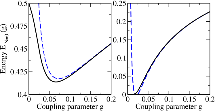
Figure 3: (color online.) The real (left panel) and the imaginary part (right panel) of the exact resonance energy of the ground state for the cubic potential are displayed as a function of $g$ (solid lines). The real part approaches the values ${\textstyle{1\over 2}}$ as $g\to 0$, whereas the imaginary part vanishes in this limit. The exact numerical values are compared to the sum of the first four leading terms of the strong-coupling asymptotics (dashed lines) for large coupling parameter $g$. The strong-coupling asymptotics are defined in Eq. (17), and the coefficients are listed in Table 2. The first four terms of the strong-coupling expansion approximate the exact resonance energies up to surprisingly small values of $g$, but both the real as well as the imaginary part deviate substantially for $g\lesssim 0.025$.

III UNIFYING STRUCTURE AND DYNAMICS

We now attempt to reconcile the structure of the cubic potential with its dynamics in a unified framework, inspired by a number of investigations regarding quantum dynamics formulated in complex coordinates Re1982arpc ; MoiseyevMcCurdy ; WiScWa2006 ; BeGaNa2007 . Notice that the construction of a time propagation algorithm from complex coordinates was explicitly mentioned as a desirable goal a rather long time ago, in Ref. Re1982arpc . Note also that the time propagation of wave packets in a cubic potential is not completely trivial: We consider a particle initially at rest and located at $q(t=0)<-(3\,\sqrt{g})^{-1}$ in the cubic potential $V(q)={\textstyle{1\over 2}}\,q^{2}+\sqrt{g}\,q^{3}$. According to classical mechanics, this particle reaches $q=-\infty$ in a finite time (as is well known), and for quantum mechanics, this means that the component of a wave packet located, loosely speaking, to the left of the cubic well is accelerated toward $q=-\infty$ by the cubic term, consistent with the Ehrenfest theorem, and escapes any (necessarily finite) grid in coordinate space used for the time propagation in a finite time. This “escape mechanism,” which leads to a loss of probability amplitude for any part of the wave packet located in a finite subinterval of coordinate space, affords a physically intuitive explanation for the finite decay width associated with the resonance eigenstates of the cubic potential.

We proceed as follows. Using a basis spanned by the standard harmonic oscillator wavefunctions $\{\phi_{J}(q)\}_{J=0}^{\infty}$, we expand the cubic eigenfunctions $\Phi_{N}(q)$ of the complex scaled Hamiltonian (13), which fulfill $H_{\rm c}(\theta)\,\Phi_{N}(q)=E_{N}\,\Phi_{N}(q)$ with complex $E_{N}$, as follows:

$$\Phi_{N}(q)\,=\,\sum\limits_{J=0}^{\infty}c_{N,J}\,\phi_{J}(q)\,.$$ (18)

Here, the complex coefficients $c_{N,J}$ are found by the diagonalization of the complex scaled Hamiltonian (13). This immediately implies that the eigenfunctions of the (dilationally–transformed) cubic potential are also complex. In Fig. 4, for example, we display the real and imaginary parts of the eigenfunctions of the ground ($N$ = 0) and excited ($N$ = 2) states of the cubic potential with $\sqrt{g}$ = 0.1.

After the evaluation of the eigenfunctions (18), the question may arise whether these function form a complete basis set. In fact, such a question is not completely trivial: it is known MoCeWe1978 ; MoFr1980 ; MoiseyevMcCurdy that for very special values of the dilational parameter $\theta$, an incomplete basis of the Hamiltonian can be obtained (see Sec. 2.5 of Ref. MoiseyevMcCurdy ). In particular, it can be shown that for special, isolated values of $\theta$, the number of linearly independent vectors of the complex-scaled potential may be smaller than the size of the Hamiltonian matrix. We note, however, that any infinitesimally small variation of $\theta$ turns the spectrum into a complete one MoiseyevMcCurdy . Below, therefore, we assume that the set of eigenfunctions (18) form a complete orthonormal basis in the complex–transformed space. That is, they fulfill the condition:

$$\left(\Phi_{N}|\Phi_{M}\right)=\delta_{NM}\,,$$ (19)

where $\left(\cdot|\cdot\right)$ is the so–called $c$–inner product introduced by N. Moiseyev and coworkers MoCeWe1978 ; MoiseyevMcCurdy :

$$\left(\Phi_{N}|\Phi_{M}\right)\,=\,\int\Phi_{N}(q)\,\Phi_{M}(q)\,{\rm d}q\,.$$ (20)

In order to illustrate the properties of the $c$-inner product, we represent the Schrödinger equation as a matrix eigenvalue problem MoiseyevMcCurdy with a Hamiltonian matrix $\bm{H}$, which we denote in boldface notation in order to emphasize that it refers to the matrix obtained after the complex rotation. In such a representation, the “bra” and “ket” eigenstates of the Hamiltonian are given by the ${\bm{\Phi}}^{\cal L}_{j}$ and ${\bm{\Phi}}^{\cal R}_{j}$ row and column eigenvectors which satisfy the matrix equations

$${\bm{H}}{\bm{\Phi}}^{\cal R}_{j}=E_{j}{\bm{\Phi}}^{\cal R}_{j}\,,$$ (21)

and

$$\left({\bm{\Phi}}^{\cal L}_{j}\right)^{\rm t}{\bm{H}}=\left({\bm{H}}^{\rm t}\,{\bm{\Phi}}^{\cal L}_{j}\right)^{\rm t}=E_{j}\left({\bm{\Phi}}^{\cal L}_{j}\right)^{\rm t}\,.$$ (22)

We recall that the eigenvalues of a matrix and its transpose are necessarily the same (as follows from the secular equation), while the corresponding left and right eigenvectors are not necessarily the same. Since the left eigenvectors ${\bm{\Phi}}^{\cal L}_{j}$ are eo ipso transposed and satisfy the eigenvalue equation of the transposed Hamiltonian, it is not necessary to invoke complex conjugation in the definition of the inner product (20). When the Hamiltonian matrix is derived from an originally “purely real” Hamiltonian such as (1) by complex scaling and thus symmetric (${\bm{H}}={\bm{H}}^{\rm t}$), then the right and left vectors are identical, ${\bm{\Phi}}^{\cal L}_{N}={\bm{\Phi}}^{\cal R}_{N}\equiv{\bm{\Phi}}_{N}$. This is the case for the cubic Hamiltonian.

We now return to the eigenfunctions (18) of the cubic Hamiltonian. These wavefunctions, which form a complete basis, may be utilized for the numerical integration of the (single–particle) Schrödinger equation and, hence, for studying the dynamical evolution of the wave packet in the cubic potential. Note, however, that this packet is defined initially in the normal (i.e., not in the scaled) space. The time propagation, therefore, requires first a complex scaling of the initial wave packet:

$$\Psi(q,t=0)\to\Psi(q\,{\rm e}^{{\rm i}\,\theta},t=0)\equiv\Psi_{\rm c}(q,t=0)\,.$$ (23)

After the complex scaling, the initial wave packet can be expanded in the basis of the functions (18)

$$\Psi_{\rm c}(q,t=0)=\sum\limits_{N=0}^{\infty}b_{N}\,\Phi_{N}(q)\,,$$ (24)

where $b_{N}=\left(\Phi_{N}|\Psi_{\rm c}(t=0)\right)$. The propagation of the wave packet $\Psi_{\rm c}(q,t)$ in the complex scaled coordinates is finally given by:

$$\Psi_{\rm c}(q,t)=\sum\limits_{N=0}^{\infty}\,b_{N}\,{\rm e}^{-{\rm i}\,E_{N}\,t}\,\Phi_{N}(q)=\sum\limits_{N=0}^{\infty}b_{N}\,{\rm exp}\left(-\frac{\Gamma_{N}}{2}\,t\right)\,{\rm e}^{-{\rm i}\,{\rm Re}(E_{N})\,t}\,\Phi_{N}(q)\,.$$ (25)

After performing the time propagation, the final function $\Psi_{\rm c}(q,t)$ should be transformed back into the “normal” space, to obtain the wave function $\Psi(q,t)$. The back-transformation proceeds by a simple inversion of the replacement operation (23),

$$\Psi_{\rm c}(q,t)\to\Psi(q,t)\equiv\Psi_{\rm c}(q\,{\rm e}^{-{\rm i}\,\theta},t)\,.$$ (26)

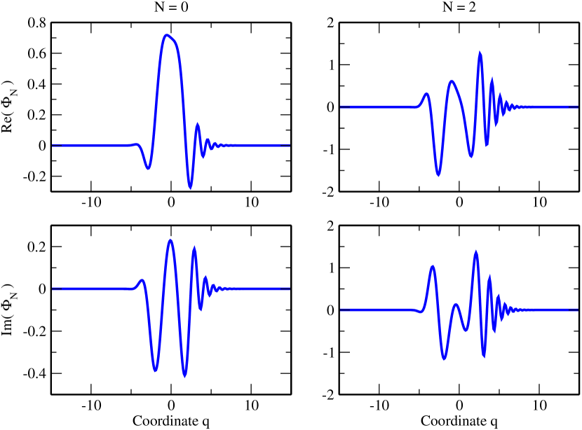
Figure 4: (color online.) Real (top panels) and imaginary (bottom panels) parts of the wavefunction $\Phi_{N}$ of the cubic Hamiltonian as a function of coordinate $q$. Results have been obtained for the ground state $N=0$ and for the second excited state with $N=2$. The coupling used is $\sqrt{g}=0.1$ and the universal complex rotation angle is $\theta=36^{\circ}$. Note that both the real and the imaginary parts of the ground-state wave function have nodes, but the wave function has no zero when considered as a complex variable.

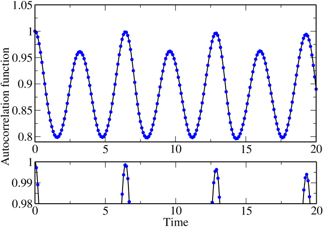
Figure 5: (color online.) Time evolution of the autocorrelation function (27). Calculations are performed for an (initially) Gaussian wave packet of the form $\Psi(q,t=0)={\rm e}^{-q^{2}}/(\pi/2)^{1/4}$ in a cubic potential with the coupling constant $\sqrt{g}=0.04$. Results obtained from Eq. (25) are compared with those of the well-known Crank-Nicolson approach (solid line). The lower panel is a close-up of the upper one, where the range of the ordinate axis in restricted to the interval $P(t)\in(0.98,1.0)$. The maximum of $P(t)=0.9939$ near the sixth oscillation, at time $t=19.29$, is faithfully reproduced by the complex scaled propagation.

Using Eq. (25), we perform calculations for the time propagation of an (initially) Gaussian wave packet within the cubic potential with the coupling parameter $\sqrt{g}$ = 0.04. In order to visualize the results of such a time propagation, we display in Fig. 5 the so–called autocorrelation function

$$P(t)=\left|\langle\Psi(t)|\Psi(0)\rangle\right|^{2}\,,$$ (27)

which is commonplace for studying tunneling phenomena in multi–well quantum dot potentials GrDiJuHa1991 . As seen from Fig. 5, the wave packet, initially located inside the well (at $q$ = 0), performs oscillations confined within the well. With every cycle of the oscillation, however, the autocorrelation function slightly decreases due to tunneling. We have also verified numerically that the decay of a wave packet corresponding to a single resonance eigenstate is described correctly by the back-transformation (26), via a comparison to a Crank-Nicolson method, where the spatial box had to be chosen sufficiently large in the latter case to accommodate the spreading of the wave packet for larger propagation times.

We note that suitable generalizations of the method (25) can also be applied to time–dependent (driven) potentials with resonances, e.g., within the adiabatic approximation, which is valid provided one uses sufficiently small time steps so that the potential can be regarded as constant in time within each time step. Recently, the adiabatic approach has been successfully applied to study the propagation of the wave packet in the driven double–well–like potential SuLuZJJe2006 .

Up to now, we have considered the idealized case of a decoherence-free, dissipation-free time evolution of the metastable states in potentials which can be approximated by a cubic Hamiltonian. The coupling of the system to an ensemble of harmonic oscillator modes, whose levels are occupied according to thermal distributions, changes the dynamics. The latter model has been studied extensively in the literature where it is commonly referred to as the Caldeira–Leggett model CaLe1981 , and it has been discussed at length in a number of research articles and books CaLe1983 ; GrWeHa1984 ; GrWe1984 ; LaOv1984 ; GrOlWe1987 ; CaIm1998 ; ClMaCl1988 ; In1997 ; We1999 ; therefore its details are relegated to the Appendix A. The model describes dissipation and the corresponding quantum decoherence, and, in general, leads to multiplicative corrections to the decay widths of the resonance eigenstates, of the form

$$\Gamma_{N}\to\Gamma_{N}\,(1+\delta_{N})$$ (28)

for the decay widths. The corrections $\delta_{N}$, initially, could be assumed as affecting only the structure of the resonance energies, but using our time propagation, it is easy to include them into the dynamics as well, by simply applying the replacement (28) to the $\Gamma_{N}$ which are present in Eq. (25).

IV SUMMARY AND OUTLOOK

In this paper, we have illustrated a certain duality of the cubic anharmonic oscillator; for purely imaginary coupling, the eigenenergies are real, whereas for real coupling, the resonance energies are complex (see Secs. II.1 and II.2). Moreover, for imaginary coupling, there are no instanton configurations to consider, and the quantization condition involves only the “perturbative $B$ function,” suitably resummed, and is of the plain Bohr–Sommerfeld type [see Eq. (7)]. By contrast, for real coupling, there are instanton configurations present, and these manifest themselves in nonvanishing decay widths of the state and in a modified quantization condition with allowance for the instanton configurations. The modified quantization is not obtained here, but we lay the groundwork for its construction. [Specifically, the leading term of the “instanton $A$ function” is given in Eq. (12).]

In other words, even anharmonic oscillators (quartic, sextic, etc.), for real coupling, are described by a plain Bohr–Sommerfeld quantization condition, whereas for negative coupling, they give rise to instantons. The structure of an even oscillator for negative coupling is thus in a certain sense analogous to an odd oscillator for real coupling $\sqrt{g}\in\mathbbm{R}$, and the presence of instantons and the corresponding nontrivial saddle points of the Euclidean action demand a modification of the Bohr–Sommerfeld quantization condition. By contrast, an even oscillator for positive coupling parameter is analogous to an odd oscillator for purely imaginary coupling $\sqrt{g}={\mathrm{i}}\,\beta$ and is described by a plain Bohr–Sommerfeld quantization condition and completely characterized by Rayleigh–Schrödinger perturbation theory.

For the determination of the resonance energies of the cubic potential (positive coupling, see Sec. II.2), three different methods have been compared. Method I (numerical approach in complex coordinates) is found to be more universal in applicability than method II (resummed weak-coupling expansion) and method III (strong-coupling expansion), although good agreement is observed in the specified domains of applicability for each of the latter two methods. In any case, the numerical approach provides us with resonance energies and corresponding wave functions in complex space which can be used in order to unify the analysis of the structure and of the dynamics of quantal particles. Hereby, the immediate physical interpretation of the decay widths can be illustrated in a particularly clear way by investigating the time propagation of wave packets.

As shown in Sec. III, the complex rotated eigenfunctions evolve in time according to complex resonance energies which describe the quantum tunneling and the decay of the wave packets. When transformed back into real space, the algorithm leads to results which are in agreement with traditional quantum dynamics solvers like the Crank-Nicolson method. The structure and the dynamics of the potentials are thus obtained in a single, unified method which allows for an inclusion of modifications to the widths of the resonances due to dissipation (coupling to the environment). For large propagation times, our algorithm is numerically stable, because the time evolution of the resonance eigenstates given by Eq. (25) remains valid for the entire coordinate space. The “escape” of the wave packet toward $q\to-\infty$, which is more pronounced for the cubic potential than, e.g., for the linear ponderomotive potential known from laser physics, is thus automatically incorporated into our algorithm. Moreover, slight modifications of the structural properties of the resonances due to additional perturbations (e.g., couplings to an environment) can easily be incorporated into the dynamics, as exemplified by Eq. (28) and discussed in more detail in Appendix A below.

V ACKNOWLEDGMENTS

U.D.J. acknowledges support from the Deutsche Forschungsgemeinschaft (Heisenberg program) and helpful discussions with Professor O. Nachtmann.

Appendix A DISSIPATION IN QUANTUM TUNNELING

Recently, a rather large number of theoretical StEtAl2003 ; MaEtAl2003prb ; BuEtAl2003prl ; GeCl2005 as well as experimental MaEtAl2002 ; BeEtAl2003sc ; BeEtAl2003prb ; XuEtAl2005 ; KaEtAl2006 studies have been devoted to the current-biased Josephson junction since its low-lying energy levels can be used to implement a solid-state quantum bit (qubit). This qubit circuit might be considered as a conceivable basis of a scalable quantum computer. The theoretical analysis of the structure and dynamics of Josephson junction qubits can be traced back to the cubic potential, at least in the limit of a dissipation-free, or decoherence-free environment, which is an idealized scenario that is nevertheless pursued in the construction of quantum computing devices. The measurement of the qubit state utilizes the escape from the cubic potential via tunneling and thus it is important to have the dynamical aspects of related potential under control.

When we work with a plain cubic Hamiltonian, it is clear that the analysis applies only to the idealized case of a decoherence-free, dissipation-free time evolution of metastable states in potentials which can be approximated by a cubic Hamiltonian. The coupling of the system to an ensemble of harmonic oscillator modes, whose levels are occupied according to thermal distributions, changes the dynamics and can be incorporated approximately into our algorithm by the replacement (28). The so-called Caldeira–Leggett model has been studied extensively in the literature CaLe1981 ; CaLe1983 ; GrWeHa1984 ; GrWe1984 ; LaOv1984 ; GrOlWe1987 ; CaIm1998 ; ClMaCl1988 ; In1997 ; We1999 and describes dissipation and the corresponding quantum decoherence. Ideally, of course, one has no dissipation in a device used for quantum computing, and this scenario has been the focus of the current investigation. It might be worth emphasizing that our approach allows for a full access to the quantum dynamics in the limit of vanishing dissipative terms, whereas the approach originally outlined in Refs. CaLe1981 ; CaLe1983 ; GrWeHa1984 ; GrWe1984 ; LaOv1984 can be used to investigate the rate at which the system loses information about coherent quantum states in the presence of dissipation, but does not lead to a general description of the full quantum dynamics in time-dependent potentials.

In general, the coupling to other degrees of freedom leads to the phenomenon of dissipation where the energy is transferred irreversibly from the system under consideration to the environment. In the work by A. O. Caldeira and A. J. Leggett CaLe1981 , the so–called “system–plus–bath” model has been introduced to describe dissipation. Within this model, the bath (environment) is considered to be representable as a set of harmonic oscillators interacting linearly with the system under consideration (i.e., with our cubic potential). The total Hamiltonian for such a system can be written as

$$H^{\rm diss}_{\rm c} = \frac{p^{2}}{2}+\frac{1}{2}q^{2}+\sqrt{g}\,q^{3}$$ (29)

$$+\sum\limits_{i=1}^{N}\left(\frac{p_{i}^{2}}{2m_{i}}+\frac{m_{i}\omega_{i}^{2}}{2}x_{i}^{2}-qc_{i}x_{i}+q^{2}\frac{c_{i}^{2}}{2m_{i}\omega^{2}_{i}}\right)\,,$$

where the first line displays “environmentally decoupled” system, i.e. the cubic anharmonic oscillator in our case. The sum over $i$ in Eq. (29) contains the Hamiltonians for a set of $N$ harmonic oscillators which are bilinearly coupled with strength $c_{i}$ to the system. Finally, the last term represents a potential renormalization term In1997 ; We1999 .

For the practical application of Eq. (29), it is necessary to eliminate the external degrees of freedom, i.e. the bath modes labeled $1,\dots,N$. Since these are just harmonic oscillator modes, we can easily solve the equations of motion for the external degrees of freedom. In a classical framework, we can derive the equation of motion for the cubic anharmonic oscillator in the bath asIn1997 ; We1999

$$\ddot{q}+\int\limits_{0}^{t}{\rm d}t^{\prime}\gamma(t-t^{\prime})\dot{q}(t^{\prime})+q+3\sqrt{g}q^{2}=\xi(t)\,.$$ (30)

Here, the damping kernel $\gamma$ is given by

$$\gamma(t)=\sum\limits_{i=1}^{N}\frac{c_{i}^{2}}{m_{i}\omega^{2}_{i}}\cos(\omega_{i}t)\,,$$ (31)

and the fluctuating acceleration

$$\xi(t) = -\gamma(t)\,q(0)$$ (32)

$$+ \sum\limits_{i=1}^{N}c_{i}\left(x_{i}(0)\cos(\omega_{i}t)+\frac{p_{i}(0)}{m_{i}\omega_{i}}\sin(\omega_{i}t)\right)\,$$

contains the initial conditions for the bath modes.

On a fully quantum level, it is convenient to describe the decay of the metastable state coupled to environment within the path integral formalism, because harmonic oscillator modes can easily be integrated out. The analysis of dissipative quantum tunneling is naturally performed in the Euclidean space (see Refs. In1997 ; We1999 for more details). That is, after a suitable Wick rotation, the imaginary–time path integral provides a representation of the equilibrium density matrix which can be represented as

$$\rho_{\beta}(q_{i},q_{f})=\frac{1}{Z_{\beta}}\int\limits_{q(0)=q_{i}}^{q(\beta)=q_{f}}\mathcal{D}q\,\exp\left(-S^{E}[q]\right)\,,$$ (33)

where $Z_{\beta}$ is the partition function which here acts as a normalization prefactor, and $\beta=1/(k_{B}T)$ is the imaginary or thermal time (we set $\hbar=1$). The paths in the integral (33) are weighted with a phase factor that contains the effective Euclidean action for the anharmonic oscillator obtained after integrating out the modes of thermal bath CaLe1981 ; CaLe1983 ; In1997 ; We1999 and reads

$$S^{E}[q] = \int\limits_{0}^{\beta}d\tau\left(\frac{p^{2}}{2}+\frac{1}{2}q^{2}+\sqrt{g}\,q^{3}\right)$$ (34)

$$+ \frac{1}{2}\int\limits_{0}^{\beta}d\tau\int\limits_{0}^{\beta}d\tau^{\prime}k(\tau-\tau^{\prime})\,q(\tau)\,q(\tau^{\prime})\,.$$

The first term of this action is just a standard Euclidean action of the cubic Hamiltonian (1), while the second term describes the frictional influence of the environment. The temperature-dependent, nonlocal (in time) damping kernel $k(\tau-\tau^{\prime})$ may be expressed as a Fourier series (see, e.g., Refs. GrOlWe1987 ; We1999 )

$$k(t)=\frac{1}{\beta}\sum\limits_{n=-\infty}^{+\infty}\xi_{n}\exp({\rm i}\,\nu_{n}\,t)\,,$$ (35)

where the $\nu_{n}=2\pi n/\beta$ are bosonic Matsubara frequencies. Finally, we have $\xi_{n}=|\nu_{n}|\,\hat{\gamma}(|\nu_{n}|)$, where $\hat{\gamma}$ denotes the Laplace transform of the damping kernel (31).

Based on the path integral approach (33)–(35), the quantum–mechanical decay of the cubic oscillator under the influence of a heat bath environment has been studied. In particular, explicit results have been obtained which helped to understand how the tunneling rate depends on the temperature of the environment, in the presence of medium and strong damping terms GrWeHa1984 ; GrOlWe1987 ; We1999 .

References

- (1) G. Gamow, Nature (London) 123, 606 (1929).
- (2) J. Zinn-Justin and U. D. Jentschura, Ann. Phys. (N.Y.) 313, 197 (2004).
- (3) J. Zinn-Justin and U. D. Jentschura, Ann. Phys. (N.Y.) 313, 269 (2004).
- (4) The Borel summation of Rayleigh–Schrödinger perturbation theory is necessitated by the asymptotic divergence of the perturbation series, whose study (for the case of stable, , perturbations), has been initiated in Refs. BeWu1969 ; BeWu1973 .
- (5) C. M. Bender and T. T. Wu, Phys. Rev. 184, 1231 (1969).
- (6) C. M. Bender and T. T. Wu, Phys. Rev. D 7, 1620 (1973).
- (7) C. M. Bender and E. J. Weniger, J. Math. Phys. 42, 2167 (2001).
- (8) C. M. Bender, G. V. Dunne, P. N. Meisinger, and M. Ṣimṣek, Phys. Lett. A 281, 311 (2001).
- (9) C. M. Bender and S. Boettcher, Phys. Rev. Lett. 80, 5243 (1998).
- (10) C. M. Bender, S. Boettcher, and P. N. Meisinger, J. Math. Phys. 40, 2201 (1999).
- (11) C. M. Bender, D. C. Brody, and H. F. Jones, Phys. Rev. Lett. 89, 270401 (2002).
- (12) C. M. Bender, S. Boettcher, G. V. Dunne, P. N. Meisinger, and M. Ṣimṣek, e-print hep-th/0108057.
- (13) K. C. Shin, Commun. Math. Phys. 229, 543 (2002).
- (14) P. Dorey, C. Dunning, and R. Tateo, J. Phys. A 34, L391 (2002).
- (15) P. Dorey, C. Dunning, and R. Tateo, J. Phys. A 34, 5679 (2002).
- (16) P. Dorey, A. Millican-Slater, and R. Tateo, J. Phys. A 38, 1305 (2005).
- (17) J. Zinn-Justin, J. Math. Phys. 25, 549 (1984).
- (18) U. D. Jentschura and J. Zinn-Justin, J. Phys. A 34, L253 (2001).
- (19) A. Mostafazadeh, J. Math. Phys. 43, 205 (2002).
- (20) A. Surzhykov, M. Lubasch, J. Zinn-Justin, and U. D. Jentschura, Phys. Rev. B 74, 205317 (2006).
- (21) J. Zinn-Justin, Quantum Field Theory and Critical Phenomena, 3rd ed. (Clarendon Press, Oxford, 1996).
- (22) F. Pham, C. R. Acad. Sc. Paris 309, 999 (1989).
- (23) B. Candelpergher, J. C. Nosmas, and F. Pham, Approche de la Résurgence (Hermann, Paris, 1993).
- (24) L. (Ed.), Méthodes Résurgentes (Hermann, Paris, 1994).
- (25) E. Balslev and J. C. Combes, Commun. Math. Phys. 22, 280 (1971).
- (26) R. Yaris, J. Bendler, R. A. Lovett, C. M. Bender, and P. A. Fedders, Phys. Rev. A 18, 1816 (1978).
- (27) G. Alvarez, Phys. Rev. A 37, 4079 (1988).
- (28) E. Caliceti, M. Meyer-Hermann, P. Ribeca, A. Surzhykov, and U. D. Jentschura, Phys. Rep. 446, 1 (2007).
- (29) V. Franceschini, V. Grecchi, and H. J. Silverstone, Phys. Rev. A 32, 1338 (1985).
- (30) U. D. Jentschura, Phys. Rev. D 62, 076001 (2000).
- (31) E. Caliceti, J. Phys. A 33, 3753 (2000).
- (32) W. P. Reinhardt, Ann. Rev. Phys. Chem. 33, 223 (1982).
- (33) S. Wimberger, P. Schlagheck, and R. Mannella, J. Phys. B 39, 729 (2006).
- (34) T. Bergmann, T. Gasenzer, and O. Nachtmann, e-print physics/0703275.
- (35) N. Moiseyev, Phys. Rep. 302, 211 (1998); C. W. McCurdy and C. K. Stroud, Comput. Phys. Commun. 63, 323 (1991).
- (36) N. Moiseyev, P. R. Certain, and F. Weinhold, Mol. Phys. 36, 1613 (1978).
- (37) N. Moiseyev and S. Friedland, J. Comp. Phys. 22, 1621 (1980).
- (38) F. Grossmann, T. Dittrich, P. Jung, and P. Hänggi, Phys. Rev. Lett. 67, 516 (1991).
- (39) A. O. Caldeira and A. J. Leggett, Phys. Rev. Lett. 46, 211 (1981).
- (40) A. O. Caldeira and A. J. Leggett, Ann. Phys. (N.Y.) 149, 374 (1983).
- (41) H. Grabert, U. Weiss, and P. Hanggi, Phys. Rev. Lett. 52, 2193 (1984).
- (42) H. Grabert and U. Weiss, Phys. Rev. Lett. 53, 1787 (1984).
- (43) A. I. Larkin and Y. N. Ovchinnikov, JETP 59, 420 (1984).
- (44) H. Grabert, P. Olschowski, and U. Weiss, Z. Phys. B 68, 193 (1987).
- (45) D. Cohen and Y. Imry, e-print cond-mat/9807038.
- (46) A. N. Cleland, J. M. Martinis, and J. Clarke, Phys. Rev. B 37, 5950 (1988).
- (47) G. L. Ingold, In Quantum fluctuations (Les Houches LXIII lectures, Elsevier, 1997), S. Reynaud, E. Giacobino, and J. Zinn–Justin (eds.).
- (48) U. Weiss, Quantum Dissipative Sustems (World Scientific, Singapore, 1999).
- (49) F. W. Strauch, P. R. Johnson, A. J. Dragt, C. J. Lobb, J. R. Anderson, and F. C. Wellstood, Phys. Rev. Lett. 91, 167005 (2003).
- (50) J. M. Martinis, S. Nam, J. Aumentado, K. M. Lang, and C. Urbina, Phys. Rev. B 67, 094510 (2003).
- (51) O. Buisson, F. Balestro, J. P. Pekola, and F. W. J. Hekking, Phys. Rev. Lett. 90, 238304 (2003).
- (52) M. R. Geller and A. N. Cleland, Phys. Rev. A 71, 032311 (2005).
- (53) J. M. Martinis, S. Nam, J. Aumentado, and C. Urbina, Phys. Rev. Lett. 89, 117901 (2002).
- (54) A. J. Berkley, H. Xu, R. C. Ramos, M. A. Gubrud, F. W. Strauch, P. R. Johnson, J. R. Anderson, A. J. Dragt, C. J. Lobb, and F. C. Wellstood, Science 300, 1548 (2003).
- (55) A. J. Berkley, H. Xu, M. A. Gubrud, R. C. Ramos, J. R. Anderson, C. J. Lobb, and F. C. Wellstood, Phys. Rev. B 68, R060502 (2003).
- (56) H. Xu, A. J. Berkley, R. C. Ramos, M. A. Gubrud, P. R. Johnson, F. W. Strauch, A. J. Dragt, J. R. Anderson, C. J. Lobb, and F. C. Wellstood, Phys. Rev. B 71, 064512 (2005).
- (57) N. Katz, M. Ansmann, R. C. Bialczak, E. Lucero, R. McDermott, M. Neeley, M. Steffen, E. M. Weig, A. N. Cleland, J. M. Martinis, and A. N. Korotkov, Science 312, 1498 (2006).